Behavioral Biases and Informational Inefficiency in an Agent-Based Financial Market

(1)

RESEARCH OUTPUTS / RÉSULTATS DE RECHERCHE

Author(s) - Auteur(s) :

Publication date - Date de publication :

Permanent link - Permalien :

Rights / License - Licence de droit d’auteur :

Bibliothèque Universitaire Moretus Plantin

Institutional Repository - Research Portal

Dépôt Institutionnel - Portail de la Recherche

researchportal.unamur.be

University of Namur

Behavioral Biases and Informational Inefficiency in an Agent-Based Financial Market

Righi, Simone; Carletti, Timoteo; Aldashev, Gani

Publication date: 2011

Document Version

Early version, also known as pre-print

Link to publication

Citation for pulished version (HARVARD):

Righi, S, Carletti, T & Aldashev, G 2011, 'Behavioral Biases and Informational Inefficiency in an Agent-Based Financial Market'.

General rights

Copyright and moral rights for the publications made accessible in the public portal are retained by the authors and/or other copyright owners and it is a condition of accessing publications that users recognise and abide by the legal requirements associated with these rights. • Users may download and print one copy of any publication from the public portal for the purpose of private study or research. • You may not further distribute the material or use it for any profit-making activity or commercial gain

• You may freely distribute the URL identifying the publication in the public portal ?

Take down policy

If you believe that this document breaches copyright please contact us providing details, and we will remove access to the work immediately and investigate your claim.

(2)

Computational Economics manuscript No.

(will be inserted by the editor)

Behavioral Biases and Informational Inefficiency in an

Agent-Based Financial Market

Simone Righi · Timoteo Carletti · Gani Aldashev

Received: date / Accepted: date

Abstract The role of competitive markets as efficient aggregators of decentralized information

is a fundamental problem in economic theory. This paper studies the informational efficiency of a market with a single traded asset, in which agents expectation formation about future price has two kinds of deviations from rationality. First, traders have adaptive expectations, i.e. they give more importance to the past price than a rational agent. Second, the agents are subject to the confirmatory bias, i.e. they tend to discard new information that substantially differs from their priors. Taken separately, each deviation worsens the informational efficiency of the market; however, for some ranges of parameters, when the two biases are combined, they tend to mitigate each others effect (thus increasing the informational efficiency). We also study the robustness of the principal findings to alternative specifications concerning market participation, entry of new agents, and the amount of liquidity that agents hold.

Keywords informational efficiency· confirmatory bias · agent-based models · asset pricing

JEL codes: G14, D82, D84.

1 Introduction

The power of competitive markets as efficient aggregators of the decentralized information that different economic agents possess is one of the fundamental problems in economic theory. Hayek

The authors thank the National Bank of Belgium for financial support. Simone Righi

Department of Economics, University of Namur (FUNDP).

Mailing address: Department of Economics, 8 Rempart de la Vierge, 5000 Namur, Belgium. Email: E-mail: [email protected]

Timoteo Carletti

naXys - Namur Center for Complex Systems, University of Namur (FUNDP). Mailing address: 8 Rempart de la Vierge, 5000 Namur, Belgium.

Email: E-mail: [email protected]. Gani Aldashev

Department of Economics and CRED, University of Namur (FUNDP).

Mailing address: Department of Economics, 8 Rempart de la Vierge, 5000 Namur, Belgium. Email: E-mail: [email protected]

(3)

(1945) first formulated the hypothesis of informational efficiency of competitive markets. Further research analyzed this hypothesis in the case of centralized (Grossman, 1976; Wilson, 1977; Milgrom, 1981) and decentralized markets (Wolinsky, 1990; Blouin and Serrano, 2001; Duffie and Manso, 2007).

Virtually all contributions in this research area assume that economic agents are fully rational. However, recent literature in experimental financial markets (e.g. Haruvy et al., 2007) finds that the traders price expectations deviate strongly from the rational-expectations assumption. Thus, while the research cited above constitutes a useful benchmark, having a more complete knowledge about the informational efficiency of markets requires relaxing the assumption of rationality of price expectations.

In this and the companion paper (Aldashev et al. 2010) we study the performance (as an efficient information aggregator) of a competitive market in which agents expectation formation about future price of the traded asset can have two kinds of deviations from full rationality. First, traders have adaptive expectations, i.e. they give more importance to the past realized price of the asset than the fully rational agent would. Second, the agents are subject to the so-called confirmatory (or confirmation) bias: they tend to discard the new information that substantially differs from their priors.

The common sense intuition indicates that a systematic deviation from rationality (among all agents) hurts the efficiency of a competitive market, because such systematic deviations from rationality in expectation formation map, via biased trading actions of agents, into equilibrium prices that do not correctly reflect the fundamental value of the traded asset. Moreover, a larger extent of such deviation should imply less market efficiency. However, we find a surprising result that while, taken separately, each of the deviations from rationality worsens the informational efficiency of the market, for some ranges of parameters, when the two biases are combined, they tend to mitigate each others effect (thus increasing the informational efficiency).

With respect to the results found in Aldashev et al. (2010), in this paper we study the robustness of the principal findings to alternative specifications of the model concerning market participation (all agents versus only the agents that revise their expectations), entry of new agents (replacement by agents with the same initial price expectation versus ones with a randomly drawn initial expectations), and the amount of liquidity that agents hold (finite, i.e. some exit occurs, versus infinite, i.e. no exit).

2 The baseline model

In Aldashev et al. (2010) authors presented a simplified model aimed to unravel some of the price formation mechanisms in a market where agents incorporate private information from peers and public information. In the present work we analyze and discuss some of the working assumptions made in Aldashev et al. (2010) and we propose some new research directions. For the sake of completeness we hereby recall the main characteristics of the above mentioned model, addressing the interested reader to Aldashev et al. (2010).

Let us thus consider a market, where time evolves by discrete steps (hereby denoted by integer values t = 0, 1, . . . ) to mimic the opening and closure of the real market periods, and that is composed by N participants - agents - each one endowed with an initial liquidity L0> 0. During

each period, agents can trade the single asset of this market at a price (normalized to belong to the interval [0, 1]) that will be denoted by Ptin period t. This price, which is public information,

is initially fixed to some level P0that can differ from the fundamental value of the asset, in this

(4)

Every agent i can place an order to buy or short sell 1 unit of the asset, on the basis of her expectation about the price for period t, hereby denoted by P_te,i. We assume that initially on

average, agents have unbiased information about its fundamental value (more specifically the

initial price expectations of the agents is drawn from a uniform distribution in the [0, 1] interval and therefore the fundamental value of the asset is actually 1₂).

The process of formation of the expectations for the next period is the main novelty of the model with respect to previous literature, being significantly different from the standard rational-expectation benchmark. This assumption constitutes thus the main theoretical contribution of both papers since it allows to model the deviations from rationality observed in the empirical literature in a relatively simple and distributed way.

More precisely, we introduce two biases in the agents expectation formation. First, agents are allowed to influence each others through social interactions with confirmatory bias, i.e. agents exchange information about prices, but they tend to disregard price information that differs to much from their own. Second, agents give a non-zero weight to the, publicly known, past market prices. The degrees to which these two biases are present in the process of decision making of the agent are defined by the parameter σ, responsible for the degree of mind openness, and α for the degree of adaptiveness.

Finally, each agent weights both contributions to get her next period expectation, more precisely, if agent i interacts with agent j then:

P_t+1e,i = αPt+ (1− α)

  

P_te,i if P_te,i− P_te,j ≥ σ

P_te,i+P_te,j

2 otherwise

, (1)

During each period, only a fraction γ ∈ (0, 1] of the N agents, is able to update their price expectation, while the remaining one keep their own previous expectations.

Once the agent has got her price expectation, she decides to participate or not to the market, and if to be a buyer or a seller. Considering that placing an order implies a small fixed but positive transaction cost c, agent i will participate to the market according to its expected

next-period gain, i.e. if P_t+1e,i − Pt − c > 0. She will participate on the buyer side if P e,i

t+1> Ptor on

the seller side if P_t+1e,i < Pt. At the end of the period, each agent learns the price Ptat which the

trade has been settled, and the profits/loss she realizes.

The market mechanism, which sets the price, Pt, at each period, is similar to the Walrasian

auctioneer, hence the market is centralized. More precisely we assume that :

1. The hypothetical price P_t+1∗ , solution of the equation nB(x) = nS(x), i.e. the price that,

almost, equates the number of buyers and sellers at price x, is calculated. Whenever there are several solutions to this equation, P_t+1∗ will denote their average;

2. In order to take into account possible disequilibrium in the market (excess of demand or supply) we introduce a correction to this hypothetical price. The market price Pt+1will move

in the direction to eliminate excess of demand or supply, i.e.:

Pt+1= β(Pt)Pt+1∗ + (1− β(Pt))Pt. (2)

Let us observe that the disequilibrium will not disappear instantly: indeed in Eq. 2 the speed of price adjustment depends on the size of the excess demand or excess supply relative to the size of the population, i.e. β(x) =|nB(x)− nS(x)| /N1;

1 _{We avoid the shortcoming of assuming a constant β(P}

t). As discussed by LeBaron (2001), if β(Pt) is assumed

to be constant, the behavior of the simulated market is extremely sensitive to the value of β, which makes it difficult to interpret the results.

(5)

Once the price has been set, each agent participating in the market, places an order, then the number of exchanges that occurs is min{nB(Pt), nS(Pt)}. Finally each seller i updates her

liquidity by Li

t+1 = Lit+ Pt− c while each buyer by Ljt+1 = L j

t − Pt− c. If, as a result of

this procedure, agent’s liquidity dries up to zero, then that agent leaves the market and she is substituted by another agent with with liquidity L0, and with same next-period price expectation

that she initially had.

In Aldashev et al. (2010) authors analyzed in details the model, with particular attention to the market inefficiency, namely the long-run deviation of Pt from the fundamental value, as

function of the key parameters: α, σ and γ. In the present paper, we propose some interesting extensions to the original model, with the aim of testing the robustness of the results and still answering to the questions: Does the market price Ptconverge to the fundamental value of the

asset? If not, how large is the market inefficiency, namely the long-run deviation of Pt from the

fundamental value?

Moreover, we are interested in understanding :

– What happen to the market inefficiency, and to other key variables, when only agents, allowed

to update their expectations, do participate to the market ?

– How the market inefficiency does depend on the new agents insertion? More precisely, how

the previous results of Aldashev et al. (2010) are modified, if, whenever an agent leaves the market because her liquidity is negative, a new agent is introduced, whose price expectation is randomly chosen and therefore uncorrelated with the previous one?

– What happens when the main source of noise, namely the substitution of agents, is eliminated?

3 The Results

The non-linearity of the interaction between agents in presence of multiple biases makes compre-hensive analytical results beyond reach, in particular when market participants are both adaptive (α > 0) and socially interacting (σ > 0). The interested reader can find a detailed analytical treatment of the cases where agents assume extreme behaviors, i.e. α ∼ 0, α ∼ 1, σ ∼ 0 and

σ∼ 1, in Aldashev et al. (2010). Thus main analysis’ tool will hereby constituted by numerical

simulations. The cost of a trading transaction is throughout fixed to c = 0.005. We let each simulation, to run until the market price converged to an almost steady state, namely when the difference between the market prices in periods t and t + 1 is smaller than the threshold 10−6.

When otherwise specified, each agent receives initially a relatively low liquidity, L0= 10, in

such a way there is the possibility that the strategy of an agent will lead to exhaustion of her liquidity. Finally, to obtain some statistics, for each pair of values (α, σ) the market simulation is repeated 10 times.

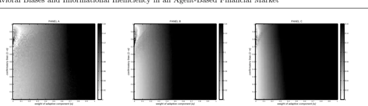
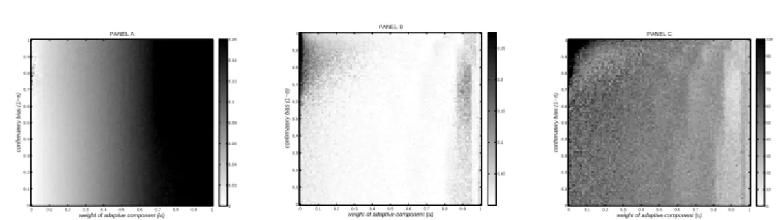
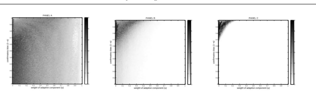
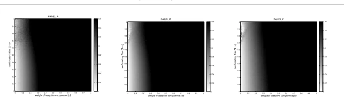
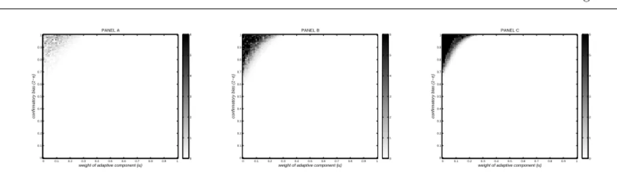
All the relevant variables have been studied as a function of the weight of the adaptive component in the price expectations of traders α and of the degree of confirmatory bias 1− σ. Figure 1 reports the informational inefficiency of the market for the cases in which the fraction of agents that revise their expectations in every period is γ = 0.2, 0.5 and 1, respectively (Panels A, B, and C where not otherwise stated). Lighter colors indicate lower level of market inefficiency, while darker ones indicate higher inefficiency. Figure 2 shows the average number of traders that exit the market as their liquidity hits the zero boundary. Figure 3 shows the standard deviation of price expectations of the agents when the market price reaches the steady state. Finally Figure 4 shows, for the case of γ = 0.2, the average liquidity owned by the agents at the end of the simulation (Panel A) together with the time needed to stabilize the market (Panel B) and the number of trades realized in the final period of the simulation (Panel C). .

(6)

weight of adaptive component (α) confirmatory bias (1− σ ) PANEL A 0 0.1 0.2 0.3 0.4 0.5 0.6 0.7 0.8 0.9 1 0 0.1 0.2 0.3 0.4 0.5 0.6 0.7 0.8 0.9 1 0 0.02 0.04 0.06 0.08 0.1 0.12 0.14 0.16

weight of adaptive component (α)

confirmatory bias (1− σ ) PANEL B 0 0.1 0.2 0.3 0.4 0.5 0.6 0.7 0.8 0.9 1 0 0.1 0.2 0.3 0.4 0.5 0.6 0.7 0.8 0.9 1 0 0.02 0.04 0.06 0.08 0.1 0.12 0.14 0.16

confirmatory bias (1− σ ) PANEL C 0 0.1 0.2 0.3 0.4 0.5 0.6 0.7 0.8 0.9 1 0 0.1 0.2 0.3 0.4 0.5 0.6 0.7 0.8 0.9 1 0 0.02 0.04 0.06 0.08 0.1 0.12 0.14 0.16

Fig. 1 Market inefficiency as a function of the adaptive component (α) and the confirmatory bias (1− σ). Panel

A: γ = 0.2, Panel B: γ = 0.5 and Panel C: γ = 1.0. Parameters are: initial price P0= 0.9, initial liquidity L0= 10,

newcoming agents have the same initial price expectation of the leaving ones.

confirmatory bias (1− σ ) PANEL A 0 0.1 0.2 0.3 0.4 0.5 0.6 0.7 0.8 0.9 1 0 0.1 0.2 0.3 0.4 0.5 0.6 0.7 0.8 0.9 1 0 1 2 3 4 5 6

confirmatory bias (1− σ ) PANEL B 0 0.1 0.2 0.3 0.4 0.5 0.6 0.7 0.8 0.9 1 0 0.1 0.2 0.3 0.4 0.5 0.6 0.7 0.8 0.9 1 0 1 2 3 4 5 6

confirmatory bias (1− σ ) PANEL C 0 0.1 0.2 0.3 0.4 0.5 0.6 0.7 0.8 0.9 1 0 0.1 0.2 0.3 0.4 0.5 0.6 0.7 0.8 0.9 1 0 1 2 3 4 5 6

Fig. 2 Average rate of exiting agents as a function of the adaptive component (α) and the confirmatory bias

(1− σ). Panel A: γ = 0.2, Panel B: γ = 0.5 and Panel C: γ = 1.0. Parameters are: initial price P0 = 0.9, initial

liquidity L0= 10, newcoming agents have the same initial price expectation of the leaving ones.

confirmatory bias (1− σ ) PANEL A 0 0.1 0.2 0.3 0.4 0.5 0.6 0.7 0.8 0.9 1 0 0.1 0.2 0.3 0.4 0.5 0.6 0.7 0.8 0.9 1 0.05 0.1 0.15 0.2 0.25 −0.20 0 0.2 0.4 0.6 0.8 1 1.2 5 10 15 20 25 30 35 40 PANEL B Price Expectation Number of agents −0.20 0 0.2 0.4 0.6 0.8 1 1.2 2 4 6 8 10 12 PANEL C Price Expectations Number of agents

Fig. 3 Panel A: Standard deviation of price expectation at convergence as a function of the adaptive component

(α) and the confirmatory bias (1− σ). Panel B: distribution of the price expectations at steady state for α = 0.01 and 1− σ = 0.9. Panel C: distribution of the price expectations at steady state for α = 0.01 and 1 − σ = 0.5. Parameters are: initial price P0= 0.9, initial liquidity L0= 10, γ = 0.2, newcoming agents have the same initial

price expectation of the leaving ones.

Proposition 1 1. The market inefficiency can be non-monotonic in (α), adaptive component

weight, and this trend is stronger, the lower is the fraction of agents that revise their price expectations in each period, i.e. small γ;

2. The slope of the relationship of market inefficiency in the degree of confirmatory bias (σ) can be of opposite sign at different values of the weight of the adaptive component (α).

3. Market inefficiency can be non-monotonic in the degree of confirmatory bias (1− σ); 4. The value of α at which the non-monotonicity of the market inefficiency with respect to the

confirmatory bias, appears gets smaller as γ increases;

5. The average liquidity is larger for parameters values giving rise to higher-than-expected inef-ficiency.

(7)

weight of adaptive component (α) confirmatory bias (1− σ ) PANEL A 0 0.1 0.2 0.3 0.4 0.5 0.6 0.7 0.8 0.9 1 0 0.1 0.2 0.3 0.4 0.5 0.6 0.7 0.8 0.9 1 10 20 30 40 50 60 70 80 90 100

confirmatory bias (1− σ ) PANEL B 0 0.1 0.2 0.3 0.4 0.5 0.6 0.7 0.8 0.9 1 0 0.1 0.2 0.3 0.4 0.5 0.6 0.7 0.8 0.9 1 0 10 20 30 40 50 60 70 80 90 100

confirmatory bias (1− σ ) PANEL A 0 0.1 0.2 0.3 0.4 0.5 0.6 0.7 0.8 0.9 1 0 0.1 0.2 0.3 0.4 0.5 0.6 0.7 0.8 0.9 1 0 50 100 150 200

Fig. 4 Average liquidity (Panel A) at convergence, time of convergence (Panel B) and number of exchanges at

steady state (Panel C) as a function of the adaptive component (α) and the confirmatory bias (1− σ). γ = 0.2. Parameters are: initial price P0 = 0.9, initial liquidity L0 = 10, newcoming agents have the same initial price

expectation of the leaving ones.

Since the results of Prop. 1.1 to 1.4 are widely analyzed in Aldashev et al. (2010) only a brief summary of the discussion on them is proposed here before proceeding with the dissertation of our new results.

The non-monotonicity with respect to α (see Prop. 1) can be observed by fixing the value of 1− σ, and moving horizontally from the left point corresponding to α = 0, to the right

α = 1 in Figure 1. The market inefficiency first decreases and then increases - at least for some

values of σ. Let us observe that, for large values of α the market inefficiency is strong, this can be explained by the fact that traders give very high weight to past prices when forming their expectations, so the initial price becomes very important. When receiving information which indicates that the value of the asset is low (whichever is the level of confirmatory bias), traders tend to disregard it - all that matters is the past price. This imply that initial price strongly influences the aggregate expectation formation process. As α declines (assuming no effective social interaction, i.e. 1−σ ∼ 1), the traders give less weight to the past prices and more weight to their expectations of the previous period. There are here two inter-related processes in action namely the upward drift of price expectations of initially low-expectation agents and the downward pressure on the market price converge, their combination lead the market price to converge not very far from the fundamental value. But when α value declines even more, market inefficiency rises again since the first process (upward move in expectations of the initially low-expectation agents) gets much slower that the second one (downward move in the market price). This leads low-expectation agents to adopt a strategy resulting in persistent negative profits, and eventually to exit the market (notice that in Figure 2 the rise in the number of agents that exit the market increases at the top-left part of the figure). This substitution of agents is sufficient to soften the downward move in the market price, resulting in higher-than-expected market inefficiency. Weakening the confirmatory bias (i.e. increasing the value of σ) the channel that leads to the exit of low expectation traders softens down, as there is now an additional mechanism that creates an upward pressure on the expectations of those traders: the integration of information that comes from their peers. However also the relationship between market inefficiency and confirmatory bias is non-monotone. As we move from the point at the bottom (σ = 0) upwards, the average deviation of the long-run market price from the fundamental value first decreases and then increases, this behaviors, summarized in Prop. 1.3 can be explained as follow: as a trader becomes more open minded, she starts to integrate at least some of the information about the fundamentals contained in the price expectations of another trader leading to lower inefficiency in the market, but when the agents becomes very open-minded (and the weight of history is not too small), this openness induce them to ’excessively’ integrate the early upward drift into the expectations, leading to higher inefficiency. Furthermore, comparing across different levels of γ

(8)

it is possible to retrieve the result of Prop. 1.4: as the fraction of agents that can update their expectations in each period (γ) increases, the area of non-monotonicity becomes smaller. This happens because the possibility to exchange information (higher γ) and the effective willingness to integrate the information coming from other traders (higher σ) act in a complementary fashion: if the possibilities to exchange information are limited, the openness of mind do not soften down the exit channel significantly. Only when the possibilities to exchange are large that the openness of mind starts to have a real bite, and the upward-sloping part on the left side of the relation between market inefficiency and alpha starts to disappear.

The area on in which the market inefficiency is higher than expected presents also an higher average level of liquidity per agent at the steady state meaning that, on average, the agents grow richer during the simulation (see Figure 4, panel A). This is the result of the combination of two effects. On the one side the time required by the market price to reach the steady state is higher (see panel B of Figure 4) when agents have low α and high (1−σ) since the agents update their expectations relatively slow. On the other side due to the large degree of confirmatory bias many interactions are rejected. This implies that agent with low initial expectation move upward slowly and, persistently underestimating the market price, effectively distribute their liquidity to the agents that where initialized nearer to the initial price. After some time this strategy dries up their liquidity and they are excluded from the market. However, these agents are substituted by other with the same initial price expectations (P₀e,i substitution) so the more time it takes to achieve equilibrium, the more the agents initially near to the market price get richer. This effect disappears when the agents give more weight to history (since the expectations of all the agents move too fast also causing a bigger inefficiency), or when the degree of confirmatory bias (1− σ) is lower (the expectations move in the direction of the market prices but, provided that the agents do not give much weight to history, the inefficiency is reduced by the mean preserving nature of social interaction as modeled here). This phenomenon is observed in all variations of this original model presented in this paper2 _{and it is summarized in Prop. 1.5.}

It is clear, from the above discussions, that the noise introduced by the exiting agents is a powerful mechanism, that alone explains a large part of the non-linear behavior of the model. To support this claim we report in Figure 5, the results of simulation with γ = 0.2 and the initial liquidity arbitrarily large (L0=∞), in this way we prevent agent from reaching the zero-liquidity

boundary and thus to leave the market. We can observe that market inefficiency (in panel A) is almost perfectly monotonic, growing with α and, to a lesser measure, with (1− σ). The non-linear effects giving rise to non monotone behaviors disappeared. The standard deviation of the expectations (Figure 5, Panel B) still increases in the area in which there was non monotonicity. This happens because the social dynamics, as described below, still divide the agents in multiple clusters of opinions. This division in groups means that some group of agents will subsidize the others but, since agents are infinitely rich, this do not have consequences on the market efficiency (no agent is ever substituted). Let us notice finally that the elimination of the noise given by the substitution of the agents do not have any significant effect on the time of convergence of the model (see Figure 5, Panel C in comparison with Figure 4, Panel B).

Let us now briefly comment on the used hypotheses. The first concerns the expectations of the newcoming agents introduced when some of the old leaves because its liquidity has reached negative values. Up to now, we assumed that the new agent has the same initial expectation of the exiting agent, namely they are strongly correlated. While this can be a reasonable assumption, for instance when the traders comes from the same company (or the same household), one cannot always assume such perfect correlation, we thus relax this assumption by allowing new entrants

(9)

confirmatory bias (1− σ ) PANEL B 0 0.1 0.2 0.3 0.4 0.5 0.6 0.7 0.8 0.9 1 0 0.1 0.2 0.3 0.4 0.5 0.6 0.7 0.8 0.9 1 0.05 0.1 0.15 0.2 0.25

confirmatory bias (1− σ ) PANEL C 0 0.1 0.2 0.3 0.4 0.5 0.6 0.7 0.8 0.9 1 0 0.1 0.2 0.3 0.4 0.5 0.6 0.7 0.8 0.9 1 0 10 20 30 40 50 60 70 80 90 100

Fig. 5 Market inefficiency (Panel A), standard deviation of the price expectations at steady state (Panel B) and

time of convergence (Panel C) as a function of the adaptive component (α) and the confirmatory bias (1− σ).

γ = 0.2. The initial price is P0= 0.9 and initial liquidity arbitrarily large L0=∞.

to have initial expectations uniformly randomly distributed, hence completely uncorrelated with that of exiting agents (for short random substitution in the following).

The second assumption is about the agents’ expectation update and the possibility to trade in the market. Up to now, we assumed that a fraction γ of agent is able to update their expectations but everybody participate to the market. While it is clearly possible that someone trade without new information, it is more realistic to assume that only people able to gather new information will take the risk of buying and selling stocks, and therefore will contribute to the formation of the market price.

3.1 Uncorrelated substitution of failed agents

The aim of this section is to study the market inefficiency under the hypothesis of random substitution, results are reported in Figures 6 to 9.

confirmatory bias (1− σ ) PANEL A 0 0.1 0.2 0.3 0.4 0.5 0.6 0.7 0.8 0.9 1 0 0.1 0.2 0.3 0.4 0.5 0.6 0.7 0.8 0.9 1 0 0.02 0.04 0.06 0.08 0.1 0.12 0.14 0.16

A: γ = 0.2, Panel B: γ = 0.5 and Panel C: γ = 1.0. Parameters are: initial price P0= 0.9, initial liquidity L0= 10,

newcoming agents have the uncorrelated initial price expectation with respect to the leaving ones.

Under this assumption, some of the previous results are confirmed: there is still non mono-tonicity with respect to weight of the adaptive component α, a behaviors that is even more marked in this case, and the area of non-monotonicity still becomes smaller as the proportion of agents that update their expectations increases. However, the market inefficiency as a function of the degree of confirmatory bias is now monotone. Hence summing up:

Proposition 2 When there is no correlation in the expectations of the agent exiting and entering

(10)

weight of adaptive component (α) confirmatory bias (1− σ ) PANEL A 0 0.1 0.2 0.3 0.4 0.5 0.6 0.7 0.8 0.9 1 0 0.1 0.2 0.3 0.4 0.5 0.6 0.7 0.8 0.9 1 0 1 2 3 4 5 6

(1− σ). Panel A: γ = 0.2, Panel B: γ = 0.5 and Panel C: γ = 1.0. Parameters are : initial price P0= 0.9, initial

liquidity L0= 10, newcoming agents have the uncorrelated initial price expectation with respect to the leaving

ones.

confirmatory bias (1− σ ) PANEL A 0 0.1 0.2 0.3 0.4 0.5 0.6 0.7 0.8 0.9 1 0 0.1 0.2 0.3 0.4 0.5 0.6 0.7 0.8 0.9 1 0.05 0.1 0.15 0.2 0.25 0.6 0.62 0.64 0.66 0.68 0.7 0.72 0.74 0.76 0.78 0.8 0 50 100 150 200 250 300 350 400 450 500 PANEL B Price expectations Number of agents

Fig. 8 Panel A: standard deviation of price expectation at convergence as a function of the adaptive component

(α) and the confirmatory bias (1− σ). Panel B: distribution of the price expectations at the steady state for

α = 0.01 and 1− σ = 0.9. In both panels γ = 0.2. Parameters are: initial price P0= 0.9, initial liquidity L0= 10,

newcoming agents have the uncorrelated initial price expectation with respect to the leaving ones.

confirmatory bias (1− σ ) PANEL A 0 0.1 0.2 0.3 0.4 0.5 0.6 0.7 0.8 0.9 1 0 0.1 0.2 0.3 0.4 0.5 0.6 0.7 0.8 0.9 1 0 10 20 30 40 50 60 70 80 90 100

confirmatory bias (1− σ ) PANEL B 0 0.1 0.2 0.3 0.4 0.5 0.6 0.7 0.8 0.9 1 0 0.1 0.2 0.3 0.4 0.5 0.6 0.7 0.8 0.9 1 0 50 100 150 200

Fig. 9 Average time of convergence (Panel A) and number of trades at the steady state (Panel B) as a function

of the adaptive component (α) and the confirmatory bias (1− σ). γ = 0.2. Parameters are: initial price P0= 0.9,

initial liquidity L0 = 10, newcoming agents have the uncorrelated initial price expectation with respect to the

leaving ones.

1. Results of Propositions 1.1, 1.2 and 1.5 are confirmed

2. Market inefficiency is monotone in the degree of confirmatory bias (1− σ), therefore Propo-sitions 1.3 and 1.4 do not hold.

3. The market price reaches the steady state while trade opportunities still exists.

In Proposition 1.3 the non-monotonicity was emerging as a result of the ’over-integration’ of the initial upward drift from the agents. The mechanism of random substitution implies that the agents with initial low expectation are much more likely to exit the market than those with high initial expectations and therefore, in the long run, there will be proportionally more of the latter

(11)

than of the former, the market price will therefore stabilize around a value farther away from the fundamental value than in the P₀e,i substitution case. Interestingly the random substitution induces a sort of natural selection of the agents, selecting those who begin nearer to the IPO price of the asset. Moreover, as for every evolutionary mechanism in a stable environment, the longer is the simulation the stronger will be its effect.

Figures 9 (Panel B) and 4 (Panel C), shows the average number of trades actions in the period in which the model reach the steady state. In the areas characterized by non monotonicity there is still activity on the market (as summarized in proposition 2.3). The reason for which the price stabilizes while there is still trade is the following: in this area agents are, almost purely, social agents, that give very little importance to historical price, and that interact through the bounded confidence mechanism that has been described. It has been shown by Weisbuch et al. (2002) that in an opinion dynamics as this one, the number of cluster formed by the agents in the long run varies as the integer part of 1

2σ. This means that agents will tend to form multiple clusters

when σ is small. Inside each cluster there is consensus on the market price, while persistent difference will remain among agents belonging to different clusters. The substitution mechanism employed is not neutral to the strength of this phenomena. If ’P₀e,i substitution’ mechanism is used then, since the agents don’t move far from their original ideas about the price before eventually exit the market the new agents substituting them will not have initial expectations significantly different from the one of those who just exit and will therefore end up in the same cluster as them (as can be seen from Figure 3, Panel B) At the opposite with the ’Random substitution’ the division in clusters will tend to disappear as a result of the evolutive selection that characterize this mechanism (see Figure 8 Panel B). Finally let us notice that the division in cluster also disappears when the degree of confirmatory bias is reduced (see Figure 3, Panel C)

3.2 Only active agents can trade

Due to the technological level of the exchange procedures employed in modern markets, everyone can set an order, thus we can suppose that also agents, unable for some practical reasons to get informed, can participate to the trade. Practically, anyway, this is not very realistic: no trader would decide to buy or sell assets without having acquired (or at least tried given time constraints that he has) as much information as possible on the asset is going to trade. Thus more realistically we assume that only those agents i that have the opportunity to update their expectation, a fraction γ of the total, do participate in the market and therefore contribute to the formation of the market price.

Figure 10, that reports the market inefficiency, clearly shows that some points of the Propo-sitions 1 and 2 still holds, while some others have to be rejected. It follows this proposition:

Proposition 3 When only active agents participate to the process of formation of the market

price:

1. Propositions 1.1 (first part), 1.2,1.3 and 1.5 hold.

2. The tendency of the market inefficiency to be non-monotonic in α is stronger, the higher is the fraction of agents that revise their price expectations in each period.

3. The weight of the adaptive component in the expectations (α) at which the non-monotonicity of the market inefficiency in the degree of confirmatory bias appears remains unchanged when the fraction of agents that revise their expectations increases.

(12)

A: γ = 0.2, Panel B: γ = 0.5 and Panel C: γ = 1.0.Parameters are: initial price P0= 0.9, initial liquidity L0= 10,

newcoming agents have the same initial price expectation of the leaving ones; only active agents contribute to the formation of the market price.

The difference between Prop 1.1 (second part) and Prop. 3.2 is the most important one. The relationship between γ, the fraction of agents allowed to update their expectations each step, and the strength of the non-linearities in α and σ is reversed. While for γ = 0.2 is almost invisible, increasing the value of this parameter the area becomes more well defined. This depends on the sensibility of the market price to the expectations of the agents, that influence it. When γ is small only a few, randomly selected, agents trade and therefore the market price will be more sensible to their choices. To understand why the non-monotonicity in the top-left part of Figure 10 (Panel A), almost disappears, remember that the population of the agent begin the simulation uniformly distributed. A random selection on such a sample will therefore tend to select agents from 0 to 1 more or less uniformly; when this is associated with the slow movement of expectations that characterize the area of non-monotonicity (low weight of history and high confirmatory bias) the consequence is that the price of the asset moves rapidly near the its fundamental value. Consistently, Figure 11 shows that more agents leave the market when γ is increased.

At the opposite the weight of the adaptive component in the expectations (α) at which the non-monotonicity of the market inefficiency in the degree of confirmatory bias appears remains unchanged regardless to γ. To understand why this happen remember that the non-monotonicity in the degree of confirmatory bias appears, in the baseline model, when the upward drift of the expectations of the low-expectation agents becomes too slow with respect to the downward movement of the market price and that both these mechanisms are influenced by the proportion of active agents each step (γ). In the present case, at the contrary, the market price become more sensible when γ is low but this do not influence significantly the movement of expectations (which depends only on α and σ, both small in the area interested by the phenomenon), the two effects actually completely offset each other leading to the result of Prop 3.3.

Observing Figure 10, in comparison with Figure 1, it is clear that while the baseline model presents values higher than 0.16 (to which we have rescaled all the images in order to make them comparable) only for high values of α now, with the exception of the area of non monotonicity, the levels of inefficiency (given some α, σ and γ) are generally higher. The reason for this is that when more agents participate to a market there is an higher volume of potential trade, which in turns leads to more efficiency. Consistently comparing the Figure 2 and Figure 11 we can see that there are more agents exiting the market (proportionally to the level of γ) in the first figure than in the second, because we now have less interactions and therefore less agents dry up their liquidity even in a larger number of steps.

Finally, looking at Figures 9 (Panel A) and Figure 12: when γ is small the simulations where all the agent participate to the market price formation process takes much more time to converge that the case in which only active people interact. The sensibility of the market price is once again

(13)

weight of adaptive component (α) confirmatory bias (1− σ ) PANEL A 0 0.1 0.2 0.3 0.4 0.5 0.6 0.7 0.8 0.9 1 0 0.1 0.2 0.3 0.4 0.5 0.6 0.7 0.8 0.9 1 0 1 2 3 4 5 6

(1− σ). Panel A: γ = 0.2, Panel B: γ = 0.5 and Panel C: γ = 1.0. Parameters are: initial price P0= 0.9, initial

liquidity L0= 10, newcoming agents have the same initial price expectation of the leaving ones; only active agents

contribute to the formation of the market price. The data have been normalized in order to control for the fact that more people participate to the market each turn (caeteris paribus) when γ is bigger.

confirmatory bias (1− σ ) PANEL A 0 0.1 0.2 0.3 0.4 0.5 0.6 0.7 0.8 0.9 1 0 0.1 0.2 0.3 0.4 0.5 0.6 0.7 0.8 0.9 1 0 10 20 30 40 50 60 70 80 90 100

confirmatory bias (1− σ ) PANEL B 0 0.1 0.2 0.3 0.4 0.5 0.6 0.7 0.8 0.9 1 0 0.1 0.2 0.3 0.4 0.5 0.6 0.7 0.8 0.9 1 0 10 20 30 40 50 60 70 80 90 100

confirmatory bias (1− σ ) PANEL C 0 0.1 0.2 0.3 0.4 0.5 0.6 0.7 0.8 0.9 1 0 0.1 0.2 0.3 0.4 0.5 0.6 0.7 0.8 0.9 1 0 10 20 30 40 50 60 70 80 90 100

Fig. 12 Average time of convergence as a function of the adaptive component (α) and the confirmatory bias

(1− σ). Panel A: γ = 0.2, Panel B: γ = 0.5 and Panel C: γ = 1.0.Parameters are: initial price P0 = 0.9, initial

liquidity L0= 10, newcoming agents have the same initial price expectation of the leaving ones; only active agents

contribute to the formation of the market price.

the main determinant of this behaviour. The market price is more sensible to the expectations of the active agents if they are the only to participate in the formation of the market price. The higher volatility of the prices implies shorter times of convergence associated with the higher levels of inefficiency already discussed.

4 Conclusions

This paper has analyzed the informational efficiency of a financial market in which the ex-pectation formation process of traders has two kinds of deviations from rationality (adaptive expectations and confirmatory bias). Taken separately, each deviation worsens the informational efficiency of the market; however, for some ranges of parameters, when the two biases are com-bined, they tend to mitigate each others effect (thus increasing the informational efficiency).

We have studied the robustness of the principal findings to alternative specifications concern-ing market participation, entry of new agents, and the amount of liquidity that agents hold. In particular, in order to test the pervasiveness of the role of the substitution mechanism we studied the case in which the initial expectation of the newcomers, about the real price of the asset, is a random value. We found that, while most of the predictions obtained in the previous case are confirmed, the non-monotonicity in the degree of confirmatory bias disappears due to the emergence of a selective process that favour the agents initially near the market price. In order to complete our analysis we then modified the model allowing only the price expectations of those agents that try to update their information to participate to the mechanism of formation of the

(14)

public market price. We discovered that, while all the non-monotonic behaviors observed in the baseline model persists, we have a reversal in the effect caused, on the market inefficiency, by the degree of participation in the market. The area in which the informational inefficiency is higher than what it would be expected if we had a monotonic behavior gets larger as the proportion of agents updating their expectations increases.

Our findings integrate those obtained in Aldashev et al. (2010) significantly extending the understanding of the consequences that the key assumptions of the model have on them. The well-known result that allocative efficiency can be obtained also in presence of significantly de-viations from the perfect rationality (Gode and Sunder, 1993,1997) is here extended also to the

informational efficiency. Indeed we show that multiple deviations from rationality, under some

assumptions and if present in the right mixes, can increase the informational efficiency of a market. This happens when the effect caused by the different biases tend to cancel each other out.

The main limitations of our analysis are twofold. First, agents are homogeneous in all aspects except the initial expectations about the market price. Second, the parameters of their degree of confirmatory bias are fixed. Further analyses should verify the robustness of our findings to relaxing these two assumptions. Another interesting direction for future work is experimental analysis of market price dynamics that would use our model as the blueprint. To the best of our knowledge, the existing experimental literature does not consider the possibility that traders influence each others expectations through social interactions (despite the informal evidence that this plays a key role; see Shiller, 1984). Studying the effect of such interactions on market behavior (in particular, informational efficiency) in the lab is a promising line for future research.

References

1. Aldashev, G., Carletti, T., and Righi, S. 2010. Follies Subdued: Informational Efficiency under Adaptive Expectations and Confirmatory Bias, JEBO, in press.

2. Blouin, M., and Serrano, R. 2001. A decentralized market with common values uncertainty: Non-steady states.

Review of Economic Studies 68: 323-346.

3. Brock, W.A., Durlauf, S.N., 2001. Discrete choice with social interactions, Review of Economic Studies 68, 235-260.

4. Deffuant, G., Neau, D., Amblard, F., and Weisbuch, G. 2000. Mixing beliefs among interacting agents. Advances

in Complex Systems 3: 87-98.

5. Duffie, D., and Manso, G. 2007. Information percolation in large markets. American Economic Review 97: 203-209.

6. Gode, D., and Sunder, S. 1993. Allocative efficiency of markets with zero-intelligence traders: Market as a partial substitute for individual rationality. Journal of Political Economy 101: 119-137.

7. Gode, D., and Sunder, S. 1997. What makes markets allocationally efficient? Quarterly Journal of Economics

112: 603-630.

8. Grossman, S. 1976. On the efficiency of competitive stock markets when traders have diverse information.

Journal of Finance 31: 573-585.

9. Haruvy, E., Lahav, Y., and Noussair, C. 2007. Traders’expectations in asset markets: Experimental evidence.

American Economic Review 97: 1901-1920.

10. Hayek, F. 1945. The uses of knowledge in society. American Economic Review 35: 519-530.

11. LeBaron, B. 2001. A builder’s guide to agent-based financial markets. Quantitative Finance 1: 254-261. 12. Milgrom, P. 1981. Rational expectations, information acquisition, and competitive bidding. Econometrica 49:

921-943.

13. Shiller, R. 1984. Stock Prices and Social Dynamics, Brookings Papers on Economic Activity, 2: 457-510. 14. Weisbuch, G., Deffuant, G., Amblard, F., and Nadal, J. 2002. Meet, discuss and segregate! Complexity 7:

55-63.

15. Wilson, R. 1977. Incentive efficiency of double auctions. Review of Economic Studies 44: 511-518. 16. Wolinsky, A. 1990. Information revelation in a market with pairwise meetings. Econometrica 58: 1-23.