HAL Id: hal-01460077
https://hal.archives-ouvertes.fr/hal-01460077
Submitted on 7 Feb 2017
HAL is a multi-disciplinary open access
archive for the deposit and dissemination of
sci-entific research documents, whether they are
pub-lished or not. The documents may come from
teaching and research institutions in France or
abroad, or from public or private research centers.
L’archive ouverte pluridisciplinaire HAL, est
destinée au dépôt et à la diffusion de documents
scientifiques de niveau recherche, publiés ou non,
émanant des établissements d’enseignement et de
recherche français ou étrangers, des laboratoires
publics ou privés.
Out-of-equilibrium Kondo Effect in a Quantum Dot:
Interplay of Magnetic Field and Spin Accumulation
Shaon Sahoo, Adeline Crépieux, M. Lavagna
To cite this version:
Shaon Sahoo, Adeline Crépieux, M. Lavagna. Out-of-equilibrium Kondo Effect in a Quantum Dot:
In-terplay of Magnetic Field and Spin Accumulation. EPL - Europhysics Letters, European Physical
Soci-ety/EDP Sciences/Società Italiana di Fisica/IOP Publishing, 2017, 116 (5), pp.57005.
�10.1209/0295-5075/116/57005�. �hal-01460077�
arXiv:1605.09149v2 [cond-mat.mes-hall] 26 Jan 2017
Out-of-equilibrium Kondo Effect in a Quantum Dot:
Interplay of Magnetic Field and Spin Accumulation
Shaon Sahoo1,2, Adeline Cr´epieux3 and Mireille Lavagna1,2,4 1 Universit´e Grenoble Alpes, INAC-PHELIQS - F-38000 Grenoble, France 2 CEA, INAC-PHELIQS - F-38000 Grenoble, France
3 Aix Marseille Univ, Universit´e de Toulon, CNRS, CPT - Marseille, France 4 Also at: Centre National de la Recherche Scientifique - CNRS - Grenoble, France.
PACS 72.15.Qm– Scattering mechanisms and Kondo effect
PACS 73.25.Dc– Spin polarized transport in semiconductors
PACS 73.23.-b– Electronic transport in mesoscopic systems
Abstract– We present a theoretical study of low temperature nonequilibrium transport through
an interacting quantum dot in the presence of Zeeman magnetic field and current injection into one of its leads. By using a self-consistent renormalized equation of motion approach, we show that the injection of a spin-polarized current leads to a modulation of the Zeeman splitting of the Kondo peak in the differential conductance. We find that an appropriate amount of spin accumulation in the lead can restore the Kondo peak by compensating the splitting due to magnetic field. By contrast when the injected current is spin-unpolarized, we establish that both Zeeman-split Kondo peaks are equally shifted and the splitting remains unchanged. Our results quantitatively explain the experimental findings reported in KOBAYASHI T. et al., Phys. Rev. Lett. 104, 036804 (2010). These features could be nicely exploited for the control and manipulation of spin in nanoelectronic and spintronic devices.
Introduction. – Progress in nano-fabrication opened the emergence of a new class of objects, semi-conductors quantum dots -QDs- in which a few electrons localized in a small spatial region are connected to leads through tun-neling barriers. QDs are very attractive for electronic and spintronic applications due to the possibility they offer to control and manipulate the spin. They give the unique op-portunity to observe a tunable Kondo effect at low temper-ature when the dot possesses an odd number of electrons and acquires a net spin S=1/2. The theoretical predic-tions of a Kondo effect in such nanostructures were made in the late 80s [1,2]. The Kondo effect is a many-body phe-nomenon which takes place when a localized impurity with an unpaired spin is embedded in a metallic host. It arises from resonant hopping processes of the conduction elec-trons of the host in and out of a localized impurity. This resonant process leads to the screening of the spin of the localized electrons with the formation of a Kondo singlet state. The binding energy of this singlet state defines the Kondo temperature TK. It was predicted that the Kondo effect leads to an increase of the linear conductance of the QD when temperature is lowered below TK. This feature
is the exact analog of the rise of resistivity brought by for the Kondo effect in bulk metals [3] when temperature is lowered below TK. Experimentally the first observation of the Kondo effect in QDs was made in GaAs-based two-dimensional structures in the late 90s [4, 5].
For any usefulness of nanoelectronic and spintronic de-vices, it is necessary to be able to control and manipulate the spin in these systems. In this perspective QDs are ex-cellent candidates since their properties can be tuned in a controlled way by varying voltages. They can be placed in an out-of-equilibrium situation by applying a finite source-drain voltage VD between the two leads (by convention source voltage VS is considered as the ground potential). In the case of a single-level QD connected to normal metal leads, the differential conductance gD = dID/dVD vs VD exhibits a zero-bias anomaly [6]. In the presence of a Zee-man magnetic field ∆, the Kondo peak in the differential conductance is split with a value of the splitting of the or-der of 2∆/e as discussed in [5, 7–9]. The transport prop-erties of the QD can also be changed by modifying the environment of the dot. A case of special interest in con-nection to the study presented in this Letter corresponds
Shaon Sahoo et al.
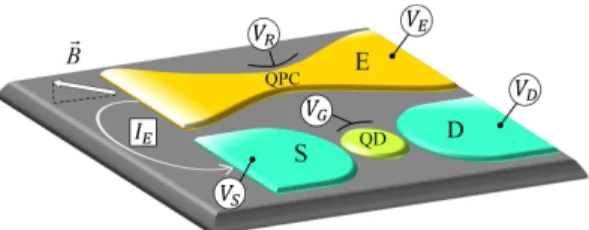
Fig. 1: Schematic representation of the experimental setup con-stituted by a QD connected to the two electrodes, source S and drain D, and a QPC responsible for the generation of the
cur-rent IE injected from the emitter E into S. An external
mag-netic field is applied to the system with the plane of the device tilted by a small angle to the axis of the magnetic field.
to QDs with ferromagnetic leads [10–13]. It was shown that spin-polarization in the leads results in an effective static magnetic field which splits the Kondo peak in gDas observed experimentally. The Kondo peak may then be restored by compensating this effective magnetic field by a Zeeman magnetic field.
More recently there has been a considerable effort in developing new techniques to modify the environment to achieve efficient control of the spin in QDs. The injec-tion of a current in one of the leads of a QD has emerged as a very powerful way to attain this goal with the pos-sibility to produce a spin accumulation in the lead when the current is spin-polarized [14–18]. We especially re-fer to experimental work by Kobayashi et al. [18] whose experimental setup is schematized in fig. 1. The genera-tion of the current is achieved with the aid of a quantum point contact -QPC- which is spin-polarized by applying a high parallel Zeeman magnetic field. The differential con-ductance of the QPC, gE = dIE/dVE vs gate voltage VR is quantized [19] at multiples of e2/h determined by the number of occupied subbands in the QPC. The current IE induced by the application of a bias voltage VE to the emitter E, is then magnetically focused [20] into S along the cyclotron trajectory by applying a low perpendicular magnetic field. In practice in order to apply a high paral-lel magnetic field for Zeeman splitting in both QPC and QD, and a low perpendicular magnetic field for magnetic focusing, the 2DEG plane is tilted by a small angle to the axis of the applied magnetic field.
The experimentalists have shown that the low temper-ature transport through a Kondo QD is considerably in-fluenced by the injection of a current into one of its leads. The observations [18] show spectacular effects on the evo-lution of the differential conductance with VD depending on the number of open transmission channels in the QPC which can be controlled by VR. The profile of the Zeeman-split Kondo peaks versus VE are found to have a very characteristic dependence on the nature of injected cur-rent. While a spin-polarized current affects the separation between the two peaks in the differential conductance, a spin-unpolarized current equally shifts both peaks. The
former case thus offers the possibility of recovering the Kondo peak by accumulating an appropriate amount of spin in one lead to compensate the Zeeman magnetic field effect.
On the theoretical side, the pioneering works go back to [17] and [21]. Qi et al. [17] examined the fate of the Kondo resonance peak in the density of states in the pres-ence of a spin accumulation for systems with a local impu-rity embedded in a metal. By using an equation of motion (EOM) approach on the single impurity Anderson model -SIAM, they found that the Kondo resonance is split into two peaks pinned to the spin-dependent chemical poten-tials. They then showed that the Kondo resonance may be restored by applying an external magnetic field. Since they are bulk, these systems do not offer the possibility of applying a finite bias voltage across the impurity. Lim et al. [21] further considered the situation of quantum dots in the presence of static spin polarization of the contact and spin accumulation in the electrode as resulting from the in-jection of a spin-polarized current. By also using an equa-tion of moequa-tion approach on the SIAM, they showed that spin polarization and spin accumulation have antagonist effects on the Kondo peak for both the spectral density and differential conductance. Whereas the spin-polarization of the contact is shown to introduce a splitting of the Kondo resonance, they demonstrated that the spin accumulation may compensate the latter splitting and restore the Kondo resonance. These two theoretical works have the merit of having highlighted the role that a spin accumulation can have on the Kondo effect. However we emphasize that their results have been obtained in the infinite U limit of the model. Moreover in [21], the truncated scheme con-sidered within the EOM approach assumes hf†
σckασi = 0 following Meir et al. [22,23]. This assumption is known to be valid in the high temperature regime when T ≥ TK. By contrast it is important to have in mind that the whole set of results obtained by Kobayashi et al. has been obtained in the low temperature regime when T ≤ TK in systems where the Coulomb interaction is estimated to 1.5meV far from the infinite U limit. The results obtained therefore in the two theoretical works do not apply to the situation in which the experiments are performed.
The purpose of this Letter is precisely to fill this dis-crepancy and to study how the spin accumulation in one of the leads of a QD affects the transport properties of an interacting quantum dot in the low temperature and finite U regime. To do this we choose to carry out our the-oretical study in conditions as close as possible to those in which the experiments were carried out. Our calcu-lations based on the single impurity Anderson model at finite U are performed by using the self-consistent renor-malized equation of motion approach following the scheme developed in [24, 25] in nonequilibrium situation. The de-coupling scheme used to truncate the set of EOM consid-ers the mixed decoupling parameter hf†
σckασi in addition to the usual decoupling parameters hc†k′α¯σckα¯σi and hn¯σi.
This additional decoupling parameter plays a key role in the description of the strong coupling regime reached at low temperature. It can be viewed as a pseudo-order pa-rameter which gets finite in the strong coupling regime, reminding of the slave-boson introduced in auxiliary-field approaches. Moreover the scheme includes two major im-provements related to the renormalization of intermediate state inverse lifetimes and the renormalization of dot en-ergy level, defining the self-consistent renormalized EOM approach. The renormalization of the intermediate state inverse lifetimes allows to cure the long-standing problem about the presence of a spurious peak in the density of states. This unphysical peak just compensates the ac-tual Kondo resonance peak at the particle-hole symmetric point εσ = −U/2, therefore prohibiting one from study-ing the Kondo physics at this point. This serious draw-back of the standard EOM approach is avoided in the self-consistent renormalized approach used in this work. Let us note that the particle-hole symmetric limit corre-sponds precisely to the situation in which the experimen-talists have conducted their experiments where the system is placed at the middle of the Kondo conductance valley. Our calculations show that the splitting of the Kondo peak in the differential conductance is modulated by the shift of the chemical potentials introduced by spin injection. The results for the differential conductance vs VDand VE are found to be in quantitative agreement with the exper-imental results. We analyze them in detail by extracting the Kondo peak parameters and comparing them with the parameters extracted from experiments.
Model. – The QD is modeled by the single impurity Anderson model H = X k,α∈(S,D),σ εkασc†kασckασ+X σ εσf† σfσ+ U n↑n↓ + X k,α∈(S,D),σ (tασc†kασfσ+ h.c.) , (1)
where c†kασ (ckασ) creates (annihilates) an electron with momentum k, spin σ (σ = ±1) and energy εkασ in the α lead. f†
σ (fσ) creates (annihilates) an electron with spin σ and energy εσ= ε0− σ∆/2 in the dot where ∆ = |g∗µBB| is the absolute value of the Zeeman splitting with g∗ the g-factor in GaAs [26] and µBthe Bohr magneton. U is the on-site Coulomb interaction in the dot. nσ= f†
σfσand tασ is the transfer matrix element between states, assumed to be k-independent.
In the steady state the current through the dot for spin σ is given by [27], IDσ = 2e ¯ h Z +W −W dωeΓσ(ω) × [nF(ω − µLσ) − nF(ω − µRσ)]Aσ(ω), (2) where eΓσ(ω) = ΓLσ(ω)ΓRσ(ω)
ΓLσ(ω)+ΓRσ(ω) with the tunnel coupling
constants given by Γασ(ω) = π|tασ|2ρ0
ασ(ω). ρ0ασ(ω) is
the density of states in the α lead for spin σ and W is the half-bandwidth. Aσ(ω) = −1πImGr
σ(ω) and Grσ(ω) are respectively the spectral density and retarded Green function in the dot. nF(ω−µασ) = [exp[(ω−µασ)/kBT )]+ 1]−1is the Fermi-Dirac distribution function in the α lead with chemical potential µασ. µDσ = µ0− eVD for both spin σ where µ0 is the chemical potential at equilibrium. When the lead S is exposed to a current injection, the chemical potentials in S are selectively shifted depending on the value of gE. When the QPC is tuned in the middle of the 0th plateau, gE = 0, no current goes through the QPC and µS↑ = µS↓ = µ0. When the QPC is tuned in the middle of the 1st plateau, gE= e2/h, a spin-polarized current with only spin-up electrons is injected into S and µS↑ = µ0− eVE whereas µS↓ = µ0. When the QPC is tuned in the middle of the 2nd plateau, gE = 2e2/h, the current is spin-unpolarized and µS↑= µS↓= µ0− eVE.
Equation of motion approach. – The spectral den-sity, Aσ(ω), appearing in eq. (2) can be derived from Gr
σ(ω) which we evaluate using the EOM approach. Ex-tensively used in the past to study bulk metals [28, 29] and quantum impurities in equilibrium [22], the EOM ap-proach has been more recently extended to nonequilib-rium [21, 23, 24, 30–35]. We use here the self-consistent renormalized EOM approach as developed in [24, 25]. In this approach the set of equations of motion of Green functions are truncated at the third level of the hierarchy by performing a decoupling in terms of all possible two-operator correlation functions with equal-spin, hfσ¯†ckα¯σi, hc†k′α¯σckα¯σi and hn¯σi where ¯σ = −σ. We point out the importance of considering the mixed decoupling param-eter hfσ¯†ckα¯σi -undeservedly neglected most often in the literature- to properly describe the strong coupling regime at low temperature. This leads to the following result [24]
Grσ(ω) = 1 − hnσi¯ ω − εσ− Σ0 σ(ω) − Π (1) σ (ω) + hn¯σi ω − εσ− U − Σ0 σ(ω) − Π (2) σ (ω) , (3) where Σ0 σ(ω) = −iσ(ω) and Γσ(ω) = P α=S,DΓασ(ω). In the wide band limit, Σ0
σ(ω) is independent of ω taking the value −iΓσ. Π(1)σ (ω) and Π(2)σ (ω) are defined as
Π(1)σ (ω) = −U Σ (1) σ (ω) − (ω − εσ)Σ(4)σ (ω) ω − εσ− U − Σ(3)σ (ω) + U Σ(4)σ (ω) ,(4) Π(2)σ (ω) = U Σ(2)σ (ω) + (ω − εσ− U )Σ(4)σ (ω) ω − εσ− Σ(3)σ (ω) + U Σ(4)σ (ω) , (5) where Σ(i)σ (ω) = X k,α |tα¯σ|2 h A(i) kασ ω + eε¯σ− eεσ− εkα¯σ+ ieγσ + A ′(i) kασ ω + eεkα¯σ− eεσ− eε¯σ− U + ieγD i , (6)
Shaon Sahoo et al. with A(1)kασ = Pk′hc † k′α¯σckα¯σi, A (2) kασ = 1 − P k′αhc † k′α¯σckα¯σi, A (3) kασ = 1, and A (4) kασ = hf † ¯ σckα¯σi/tα¯σ. A′(i)kασ= (A(i)kασ)∗ for i = 1, 2, 3 and A′(4)
kασ = −(A (4) kασ)∗. Expression (3) for Gr
σ(ω) is exact both in the non-interacting limit (U = 0) and in the isolated-site limit (tασ = 0). The expression exhibits two poles at εσ and (εσ+ U ) corresponding to the isolated-site limit, weighted by the factors (1 − hn¯σi) and hn¯σi respectively. Σ0
σ(ω) is the ordinary self-energy due to electron tunneling be-tween the dot and the leads, whereas Π(1)σ (ω) and Π(2)σ (ω) are the self-energy contributions due to interactions. Ex-pression (3) constitutes an extension of Lacroix’ [29] and Meir et al.’s [22] results. At equilibrium and in the infi-nite U limit, the expression gives back the results of [29]. When hfσ†¯ckα¯σi = 0 (and hence Σ
(4)
σ (ω) = 0), the results of [22] are recovered, corresponding to the high temperature limit. The consideration of this extra-parameter hfσckα¯¯† σi is crucial to describe the low-temperature limit. It ensures the unitary condition for Gr
σ(ω) at the Fermi level to be fulfilled at zero temperature [24, 25, 29]. The decoupling parameters hfσ¯†ckα¯σi, hc†k′α¯σckα¯σi, and hn¯σi are then de-termined by the self-consistent equations established both at and out-of-equilibrium [24] provided that the system is in a steady state. As a result the self- energies Σ(i)σ (ω) are expressed in terms of Gr
σ(ω). The Green function Grσ(ω) can then be self-consistently calculated from eq. (3).
We consider two important improvements related to the renormalization of both intermediate state inverse life-times and dot energy level. These two improvements de-fine the self-consistent renormalized EOM approach where propagators and vertices of the corresponding skeleton Feynman diagrams are dressed by self-energy and vertex corrections respectively. In the standard EOM approach, e
εσ is the bare energy level εσ in the dot, and eγσ and eγD are both an infinitesimal positive (γσ= γD= +iδ). They are renormalized in the self-consistent renormalized EOM approach. On the one hand, eεσ is renormalized by self-energy corrections according to: eεσ = εσ+ ℜΣ(1)σ (ω = eεσ). At the particle-hole symmetric point the renormalization effect on eεσ is zero and eεσ = εσ. On the other hand eγσ and eγD are replaced by the inverse lifetimes of intermedi-ate stintermedi-ates. They are determined by using the generalized Fermi golden rules up to the forth order in tασ following [24, 25], extending to finite U the argument used in [23] for the infinite-U limit. The renormalization of eγD proves to be extremely important to cure the long-standing prob-lem about the presence of a spurious peak in the density of states. This unphysical peak, which compensates the actual Kondo resonance peak, is the reason behind the failure of the standard EOM approaches. This drawback is avoided in the self-consistent renormalized EOM ap-proach used in this work. By using Eqs. (2-6), we have all the ingredients to derive the total current ID and the differential conductance gD= dID/dVD.
Choice of parameters and Kondo temperature. – Except for U , the values of all the parameters inserted in our model are adopted from the estimations made in [18]. Hence the electronic temperature is taken as T = 100 mK, ∆ = 130 µeV and Γασ = 0.25 meV. As far as U is concerned, we choose to take a slightly larger value U = 3 meV instead of U = 1.5 meV considered in [18] to ensure that the system is in the Kondo regime on the following criterion: 2Γασ ≪ U/2. Besides we consider the system at the particle-hole symmetric point with ε0 = −U/2 in agreement with the experimental situation.
The Kondo temperature, TK, of the QD is estimated from the linear conductance vs temperature plotted at equilibrium (for B = VE = 0). TK is the temperature at which the linear conductance falls down to half of its maxi-mum value. We get: TK = 0.5 K. Upper bounds to TKcan be found in various nonequilibrium situations. For exam-ple, an upper bound to TK is estimated from the value of the FWHM of the Kondo peak in gDvs VD plot. We per-form calculations at T = 100 mK (for B = VE = 0), and get TK < 0.7 K. Finally the value of TK estimated from Haldane’s formula [36] is 0.9 K. These values are consistent with the upper bound 0.7 K estimated in experiment [18] even though we have taken a slightly different value of U . Let us also mention that all our numerical calculations are performed at 100 mK, well below the estimated TK.
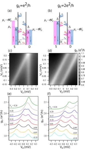
Results and discussion. – Our numerical results for the differential conductance gD are represented in both gray-scale representation in the plane (VD,VE) in figs. 2(c)-2(d), and in gDvs VDplots in figs. 2(e)-2(f) at gE= e2/h and gE = 2e2/h respectively. We do not show the result for gE = 0 since gDvs VDplot is simply the one obtained for gE 6= 0 at VE = 0. As can be seen from figs. 2(e)-2(f), generally gD vs. VD has two peaks. The variations of the positions of the peaks with VE depend on the spin-polarization state of the injected current. At VE = 0 the Kondo peaks occur at VD = ±∆/e as expected. When the injected current is spin-polarized (by tuning the QPC at gE = e2/h), the position of the upper-VD peak does not vary with VE whereas that of the lower-VD peak is linearly shifted by VE. The separation between the two peaks decreases with increasing positive VEuntil vanishing at a critical value of VE. When the injected current is spin-unpolarized (by tuning the QPC at gE= 2e2/h), the positions of both peaks are equally shifted by VE.
With the aim of understanding the physical mechanisms behind these results, we illustrate in figs. 2(a)-2(b) the schematic representation of the energy level diagram in the QD at gE = e2/h and gE = 2e2/h respectively, for finite VD, VE and ∆. From eq. (3) it is easy to see that the spectral density Aσ(ω) exhibits two Kondo peaks at about (µα¯σ+ εσ− ε¯σ) = µα¯σ− σ∆ for each α [37]. Fol-lowing eq. (2), gD vs VD exhibits a peak whenever one of the chemical potentials for a given spin gets aligned with a Kondo DOS peak for the same spin. This oc-curs when µβσ = (µα¯σ+ εσ− ε¯σ), leading to the
ana--0.15 -0.1 -0.05 0 0.05 0.1 0.15 0.2 -0.3 -0.2 -0.1 0 0.1 0.2 0.3 (null) (null) ’cndct_ge.1.out’ 0.6 0.65 0.7 0.75 0.8 0.85 0.9 0.95 1 1.05 1.1 -0.15 -0.1 -0.05 0 0.05 0.1 0.15 0.2 -0.3 -0.2 -0.1 0 0.1 0.2 0.3 (null) (null) ’cndct_ge.2.out’ -0.3 -0.2 -0.1 0.0 0.1 0.2 0.3 1.0 1.5 2.0 2.5 V E= 0.26 0.20 0.15 0.10 0.05 0.00 -0.05 -0.10 -0.3 -0.2 -0.1 0.0 0.1 0.2 0.3 1.0 1.5 2.0 2.5 VE= 0.26 0.20 0.15 0.10 0.05 0.00 -0.05 -0.10 gD (e 2/h) gD (e 2/h) gD (e2/h) VD (mV) VD (mV) VD (mV) VD (mV) VE (mV) VE (mV) (c) (d) (e) (f) S D S D (a) (b) gE=e2/h gE=2e2/h
Fig. 2: (a)-(b) Schematic representation of the energy level
diagram in the QD at gE = e2/h and gE = 2e2/h for finite
VD, VE and ∆. ρ↑ (ρ↓) represent the Kondo peaks in A↑(ω)
(A↓(ω)). (c)-(d) Results for the differential conductance gDin
gray-scale representation in the plane (VD,VE) at gE = e2/h
and gE = 2e2/h. (e)-(f) Results for the differential
conduc-tance gD vs VD at gE= e2/h and gE= 2e2/h for VE ranging
from -0.10 mV (bottom) to 0.26 mV (top). The curves are
ver-tically offset by 0.2e2/h for clarity. The results are obtained
for the symmetric Anderson model at T = 100 mK with U =
3 meV, Γασ = 0.25 meV and ∆ = 0.13 meV.
lytic prediction for the positions of the Kondo peaks. At gE = 0 the Zeeman-split Kondo peaks is found to occur at VD = ±(εσ − ε¯σ)/e = ±∆/e. The splitting is equal to 2∆/e. At gE = e2/h, the two Kondo peaks are found to be located at VD = −∆/e + VE and VD = ∆/e. The separation between these two peaks is (2∆/e − VE), which decreases with increasing VE. When VE= 2∆/e, the Zee-man splitting of the Kondo peak is exactly compensated by spin accumulation in the lead produced by the injection of a spin-polarized current. At this compensation point, the two peaks merge into a single peak and the Kondo peak is restored. This manifestation can be viewed as the fingerprint of the formation of the Kondo spin-singlet state at low temperature. At gE = 2e2/h, the analytic predictions for the positions of the two Kondo peaks are
VD = −∆/e + VE and VD = ∆/e + VE. The separation between peaks is 2∆/e, independent of VE.
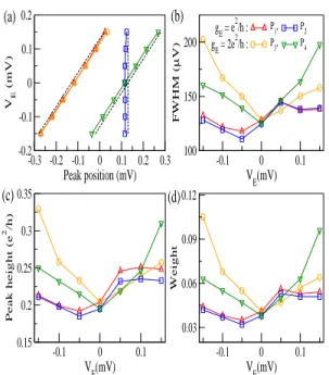
In order to extract the peak parameters from our nu-merical results, we fit the curves in figs. 2(e)-2(f) by a double-Lorentzian function with a quadratic background according to: f (x) = a+bx+cx2+z1h1
π w1/2 (x−x1)2+(w1/2)2 i + z2h1π w2/2 (x−x2)2+(w2/2)2 i
. The quadratic background is nec-essary to account for the contributions of the two broad charge peaks in the DOS. We take two different weight factors z1 and z2 to account for the asymmetry in the spectral density arising mainly from charge accumulation in S when VE6= 0. The extracted values for peak positions xi (i=1,2), FWHMs wi, heights 2zi/(πwi) and weight fac-tors zi are reported in fig. 3. It is worth noticing that the parameter extraction is possible only up to VE= 0.15 mV. Beyond this value the two peaks are too close and can no longer be resolved. As expected, wi, heights and weight factors of the two peaks coincide at VE= 0 in both cases. In fig. 3, P1 and P2 correspond respectively to the lower-VD and upper-VD peaks at gE = e2/h whereas P3 and P4 are the equivalent peaks at gE = 2e2/h. As can be seen in fig. 3(a), our numerical results for the peak po-sitions (in solid lines) are in excellent agreement with our analytical predictions of VD = VE± ∆/e and VD = ∆/e (in broken lines). The extracted FWHMs vs VE for the different peaks are reported in fig. 3(b). The values of the FWHM give us some useful information about the de-gree of decoherence in the Kondo resonance. The higher VD, ∆ or (µασ− µ0), the higher the FWHM. As can be seen from fig. 3(b), wi for both P1 and P2 saturate at large positive values of VE when the system gets closer to the compensation point where the Kondo peak is restored. From the same figure, one can see that wi for P3 and P4 do not show any evidence of saturation at large values of VE as expected. Finally the extracted peak heights and weight factors vs VE are reported in figs. 3(c)-3(d). While the peak height results from the two antagonistic effects brought by zi and 1/wi contributions respectively, the re-sults show that the dominant contribution is provided by zi.
The orders of magnitude of the various peak parame-ters and their overall evolution as a function of VE are in good agreement with the experimental data [18] although the value that we adopted for U is slightly different from the experimental estimation. However we would like to point out that unlike what we find in our calculations, the experimental results show a deflection of the P2 line from VD = ∆/e in the vicinity of the Kondo compensa-tion point along with large and sudden fluctuacompensa-tions of the FWHMs for both P1 and P2 in this range. One of the reasons for this behavior as suggested in Ref. [18] is that the system is in a highly nonequilibrium situation when gE = e2/h and hence the fermion states below µS↑ along the cyclotron trajectory from E to S, are not fully occu-pied at zero temperature [38, 39]. Ihis would result in a double-step instead of the single-step Fermi-Dirac
distri-Shaon Sahoo et al. -0.3 -0.2 -0.1 0 0.1 0.2 0.3 Peak position (mV) -0.2 -0.1 0 0.1 0.2 V E (mV) P1, P3, -0.1 0 0.1 VE(mV) 100 150 200 FWHM ( µ V) -0.1 0 0.1 VE(mV) 0.15 0.2 0.25 0.3 0.35 Peak height (e 2/h) -0.1 0 0.1 VE(mV) 0.03 0.06 0.09 0.12 Weight P2 P4 gE = e2/h : g E = 2e 2 /h : (b) (a) (c) (d)
Fig. 3: Kondo peak parameters extracted from results for gD
vs VD. (a) Peak positions. The extracted peak positions are
represented in solid lines whereas our analytical predictions
VD= VE±∆/e and VD= ∆/e are represented in broken lines.
(b) FWHMs. (c) Peak heights. (d) Weight factors.
bution function considered in our calculations. It would be interesting in the future to investigate consequences of this situation.
Conclusion. – In summary, we have studied the com-bined effects of Zeeman magnetic field and current injec-tion into one lead on the nonlinear conductance of a QD in the low temperature regime. When the injected current is spin-polarized, the Zeeman splitting of the Kondo peak in the differential conductance is found to be compensated by an appropriate amount of spin accumulation in the lead and the Kondo peak is restored in good agreement with experimental data [18]. Our results in this Letter show that the injection of a current in one lead of a QD offers a new and promising route to controlling and manipulating spin in nanoelectronic devices. Present work opens the possibility of studying other important situations such as separate spin accumulations in both leads with or without the presence of magnetic field. In the absence of magnetic field, we predict that the Kondo peak is restored when the two leads have an equal amount of spin accumulation with opposite spin orientation.
∗ ∗ ∗
We would like to thank H. Baranger for valuable discus-sions. For financial support, the authors acknowledge the Indo-French Centre for the Promotion of Advanced Re-search (IFCPAR) under ReRe-search Project No.4704-02 and the Nanosciences Foundation of Grenoble under Contract CORTRANO.
REFERENCES
[1] Ng T.K. and Lee P.A., Phys. Rev. Lett., 61 (1988) 1768. [2] Glazman L. and Raikh M., JETP Lett., 11 (1988) 2389. [3] Hewson A.P., The Kondo Problem to Heavy Fermions (Cambridge University Press) 1993 and references therein. [4] Goldhaber-Gordon D., Shtrikman H., MahaluD.,
Abusch-Magder D., Meirav U.and Kastner M.,
Na-ture, 61 (1998) 156.
[5] Cronenwett S.M., Oosterkamp T.H. and Kouwen-hoven L.P., Science, 281 (1998) 165115.
[6] van der Wiel W., De Franceschi S., Fujisawa T.,
Elzerman J., Tarucha S.and Kouwenhoven L.P.,
Sci-ence, 289 (2000) 2105.
[7] Costi T.A., Phys. Rev. Lett., 85 (2000) 1504 .
[8] Rosch A., Paaske J., Kroha J. and W¨olfle P., Phys.
Rev. Lett., 90 (2003) 076804.
[9] Hewson A.C., Bauer J. and Oguri A., J. Phys.:
Con-dens. Matter, 17 (2005) 5413.
[10] Zhang P., Xue Q.-K., Wang Y.P. and Xie X.C., Phys.
Rev. Lett., 89 (2002) 286803.
[11] Martinek J., Utsumi Y., Imamura H., Barna´s J.,
Maekawa S., K¨onigand Sch¨oJ.G., Phys. Rev. Lett., 91
(2003) 127203 .
[12] Choi M.-S., S´anchez D.and L´opez R., Phys. Rev. Lett.,
92(2004) 056601.
[13] Krawiec M., J. Phys.: Condens. Matter, 19 (2007) 346234.
[14] Potok R.M., Folk J.A., Marcus C.M. and Umansky V., Phys. Rev. Lett., 89 (2002) 266602.
[15] Taniyama T., Fujiwara N., Kitamoto Y. and Ya-mazaki Y., Phys. Rev. Lett., 90 (2003) 016601.
[16] Katsura H., J. Phys. Soc. Jpn., 76 (2007) 054710. [17] Qi Y., Zhu J.-X., Zhang S. and Ting C.S., Phys. Rev.
B, 78 (2008) 045305.
[18] Kobayashi T., Tsuruta S., Sasaki S., Fujisawa T.,
Tokura Y.and Akazaki T., Phys. Rev. Lett., 104 (2010)
036804.
[19] van Wees B.J., Kouwenhoven L.P., van Houten H.,
Beenakker C.W.J., Mooij J.E., Foxon C.Tand
Har-ris J.J., Phys. Rev. B, 38 (1988) 3625.
[20] van Houten H., Beenakker C.W.J., Williamson J.G., Broekaart M.E.I., van Loosdrecht P.H.M.,
van Wees B.J., Mooij J.E., Foxon C.T. and Harris
J.J., Phys. Rev. B, 39 (1989) 8556.
[21] Lim J.S., L´opez R., Limot L.and Simon P., Phys. Rev.
B, 88 (2013) 165403.
[22] Meir Y., Wingreen N.S. and Lee P.A., Phys. Rev.
Lett., 66 (1991) 3048.
[23] Meir Y., Wingreen N.S. and Lee P.A., Phys. Rev.
Lett., 70 (1993) 2601.
[24] Lavagna M., Journal of Physics: Conference Series, 592 (2015) 012141.
[25] Lavagna M., Nonequilibrium quantum transport through
an interacting quantum dot, in preparation.
[26] Note the minus sign in front of σ∆/2 in the expression of
εσ due to the fact that g∗= −0.44 in GaAs.
[27] Meir Y. and Wingreen N.S., Phys. Rev. Lett., 68 (1992) 2512.
[28] Appelbaum J.A. and Penn D.R., Phys. Rev. B, 188 (1969) 874.
[30] Entin-Wohlman O., Aharony A. and Meir Y., Phys.
Rev. B, 71 (2005) 035333 .
[31] Monreal R.C. and Flores F. , Phys. Rev. B, 72 (2005) 195105.
[32] Kashcheyevs V., AharonyA. and Entin-Wohlman O., Phys. Rev. B, 73 (2006) 125338.
[33] ´Swirkowicz R., Wilczy´nski M. and Barna´s J., J.
Phys.: Condens. Matter, 18 (1988) 2006.
[34] Qi Y., Zhu J.X. and Ting C.S., Phys. Rev. B, 79 (2009) 205110 .
[35] Van Roermund R., Shiau S.Y. and Lavagna M. , Phys.
Rev. B, 81 (2010) 165115.
[36] Haldane F.D.M., Phys. Rev. Lett., 40 (1978) 416. [37] The fact that the Kondo peak in the density of states
Aσ(ω) occurs at (µα ¯σ−σ∆) reflects the formation of the
Kondo spin-singlet state at low temperature.
[38] De Franceschi S., Hanson R., van der Wiel W.G., Elzerman J.M., Wijpkema J.J., Fujisawa T.,
Tarucha S.and Kouwenhoven L.P., Phys. Rev. Lett.,
89(2002) 156801.
[39] Pothier H., Gu´eron S., Birge N.O., Est`eve D. and