HAL Id: tel-00759059
https://tel.archives-ouvertes.fr/tel-00759059
Submitted on 1 Dec 2012HAL is a multi-disciplinary open access archive for the deposit and dissemination of sci-entific research documents, whether they are pub-lished or not. The documents may come from teaching and research institutions in France or abroad, or from public or private research centers.
L’archive ouverte pluridisciplinaire HAL, est destinée au dépôt et à la diffusion de documents scientifiques de niveau recherche, publiés ou non, émanant des établissements d’enseignement et de recherche français ou étrangers, des laboratoires publics ou privés.
programming with first-order syntax with binders
Nicolas Pouillard
To cite this version:
Nicolas Pouillard. Namely, Painless: A unifying approach to safe programming with first-order syntax with binders. Programming Languages [cs.PL]. Université Paris-Diderot - Paris VII, 2012. English. �tel-00759059�
Universit´
e Paris Diderot (Paris 7)
´
Ecole doctorale : Sciences Math´
ematiques de
Paris Centre
DOCTORAT
Informatique
Une approche unifiante pour programmer
sˆ
urement avec de la syntaxe du premier
ordre contenant des lieurs
english title:
Namely, Painless
A unifying approach to safe programming with
first-order syntax with binders
Nicolas Pouillard
Th`ese dirig´ee par Fran¸cois Pottier
et soutenue le 13 Janvier 2012 devant le Jury compos´e de : Pr´esident M. Roberto Di Cosmo
Rapporteurs M. Andrew Pitts M. Dale Miller Examinateurs M. Daniel Hirschkoff
M. Conor McBride Directeur M. Fran¸cois Pottier
`
Abstract
This dissertation describes a novel approach to safe meta-programming. A meta-program is a program which pro-cesses programs or similar data. Compilers and theo-rem provers are prime examples of meta-programs which could benefit from this approach. To this end, this work focuses on the representation of names and binders in data structures.
Programming errors are really easy to make with usual techniques. We propose an abstract interface to names and binders that rules out these errors. This interface is implemented as a library in Agda. It allows defining and manipulating term representations in nominal style. Thanks to abstraction, other styles are supported as well: the de Bruijn style, the combinations of these styles, and more.
Whereas indexing the types of names and terms with a natural number is a well-known technique to better control de Bruijn indices, we index them with worlds. Worlds are at the same time more precise and more ab-stract than natural numbers. Via logical relations and parametricity, we are able to demonstrate in what sense our library is safe, and to obtain theorems for free about world-polymorphic functions. For instance, we prove that a world-polymorphic term transformation function must commute with any renaming of the free variables. The proof is entirely carried out in Agda.
The usability of our technique is shown on several ex-amples including normalization by evaluation which is known to be challenging. We show that our world-indexed approach can express a wide range of data types by embedding several definition languages from the liter-ature.
5 R´esum´e
Cette th`ese d´ecrit une nouvelle approche pour la m´ eta-programmation sˆure. Un m´eta-programme est un pro-gramme qui manipule des propro-grammes ou assimil´es. Les compilateurs et syst`emes de preuves sont de bons exemples de m´eta-programmes qui b´en´eficieraient de cette approche. Dans ce but, ce travail se concentre sur la repr´esentation des noms et des lieurs dans les structures de donn´ees.
Les erreurs de programmation ´etant courantes avec les techniques usuelles, nous proposons une interface abs-traite pour les noms et les lieurs qui ´elimine ces er-reurs. Cette interface est impl´ement´ee sous forme d’une biblioth`eque en Agda. Elle permet de d´efinir et manipu-ler des repr´esentations de termes dans le style nominal. Grˆace `a l’abstraction, d’autres styles sont aussi dispo-nibles : le style de De Bruijn, les combinaisons de ces styles, et d’autres encore.
Nous indi¸cons les noms et les termes par des mondes. Les mondes sont en mˆeme temps pr´ecis et abstraits. Via les relations logiques et la param´etricit´e, nous pouvons d´emontrer dans quel sens notre biblioth`eque est sˆure, et obtenir des “th´eor`emes gratuits” `a propos des fonc-tions polymorphiques. Ainsi une fonction monde-polymorphique de transformation de termes doit commu-ter avec n’importe quel renommage des variables libres. La preuve est enti`erement conduite en Agda.
Notre technique se montre utile sur plusieurs exemples, dont la normalisation par ´evaluation qui est connue pour ˆ
etre un d´efi. Nous montrons que notre approche indic´ee par des mondes permet d’exprimer un large panel de type de donn´ees grˆace a des langages de d´efinition embarqu´es.
Remerciements
Trois ann´ees de noms et de termes. Des liens puis des noms, des noms et des indices, puis des indices seulement, puis finalement encore des noms. Aujourd’hui j’´ecris ces remerciments et ce sont vos noms qui me viennent `a l’esprit.
Je porte mes remerciements tout d’abord `a ma famille, mes parents, pour m’avoir soutenu dans mes longues ´etudes. Merci aussi `a mon ´epouse, Ga¨elle, qui m’a non seulement soutenu mais ´epaul´e, ´ecout´e, pouss´e, aid´e, ... Bref, elle est aussi responsable de cet aboutissement.
Je tiens particuli`erement `a remercier mes relecteurs pour leur travail remarquable. Leurs relectures de ce document m’ont permis de nombreuses am´eliorations rendant le pr´esent document plus accessible et plus complet.
Je remercie le LRDE qui m’a aiguill´e vers la recherche, je remercie en particulier Akim Demaille pour son cours de compilation qui m’a initi´e `a la conception de langages.
Je remercie d’avance tous ceux que je ne mentionne pas individuelle-ment ici : membres de ma famille, camarades, coll`egues, ami(e)s, simples connaissances. Vous qui justement lisez ces lignes, je vous en remercie.
Un grand merci `a toute l’´equipe Gallium de l’INRIA Rocquencourt et tous les membres que j’y ai rencontr´es. Cette ´equipe m’a accueilli jeune ing´enieur et m’a rendu jeune chercheur. Plus particuli`erement je remercie : Michel Mauny pour m’avoir accept´e en stage mais aussi sur le contrat qui a suivi ; j’y ai appris une foule d’anecdotes sur l’´evolution des dialectes succes-sifs de Caml ; grˆace `a lui et malgr´e lui j’ai appris `a appr´ecier la programma-tion paresseuse (sans jeux de mots) ce qui m’a ouvert de nouveaux horizons. Puis c’est au tour de Fran¸cois Pottier, qui m’a accept´e en th`ese et m’a ha-bilement guid´e et soutenu pendant ces ann´ees. Il a su ˆetre disponible et `a l’´ecoute. Outre une montagne de connaissances scientifiques, j’ai appris de lui l’art d’´ecrire des articles bien que j’ai encore beaucoup `a apprendre `a ce sujet. Xavier Leroy pour son accueil et sa bienveillance quant `a la bonne marche de l’´equipe ; Damien Doligez pour son intarissable culture et ses th´eories sur tout ; Didier R´emy pour ses discussions sur les d´etails du fonctionne-ment de TEX :) ; Alain Frisch pour m’avoir enseign´e tellefonctionne-ment de choses sur OCaml et la programmation fonctionnelle en g´en´eral pendant les mois du-rant lesquels j’ai partag´e son bureau ; Yann R´egis-Gianas pour avoir trac´e
une voie qu’il m’a suffit d’emprunter ; Berke Durak pour m’avoir accom-pagn´e dans le d´eveloppement d’ocamlbuild ; Benoit Razet pour toutes nos discussions sur les automates et les structures de flots de donn´ees ; G´erard Huet pour ses anecdotes vari´ees qui m’ont beaucoup appris ; Jean-Baptiste Tristan pour avoir particip´e et accueilli chez lui l’´equipe des “jeunes” de Gal-lium au concours ICFP ; Tous ceux qui ont particip´e aux concours ICFP ; Arthur Chargu´eraud pour son secret de l’efficacit´e : les axiomes Coq et notepad++:) ; Zaynah Dargaye, Boris Yakobowski et Paolo Herms pour les discussions et les bons moments pass´es avec eux ; Benoˆıt Montagu pour m’avoir ouvert son bureau et avoir partag´e des discussions fructueuses sur nos th`eses respectives ; Julien Cretin pour sa singularit´e mais aussi pour tous les sujets sur lesquels nous pouvons discuter agr´eablement ; Alexandre Pilkiewicz de m’avoir traˆın´e jusqu’au parcours sportif un certain nombres de fois ; Jonathan Protzenko car grˆace `a lui le web ´evolue de jour en jour :) ; Tahina Ramananandro pour nos discussions politiques et nos concours de jeux de mots fumeux ; Dana Xu pour ses encouragements ; Gabriel Scherer et Valentin Robert pour leurs nombreux commentaires sur des parties de ce document.
`
A Luc Maranget pour les discussions nautiques et ses slogans devenus cultes : “Les programmeurs veulent des types plus riches !”, “Les types exis-tentiels existent-ils ?”, “Ils nous parlent seulement des types, o`u sont les termes ?” ; Jean-Jacques Levy pour son talent `a poser tout haut les ques-tions auxquelles tout le monde pense.
J’ai une pens´ee aussi pour tous les “camarades de navette” avec qui j’ai pu discuter pendant un des nombreux trajets entre Paris et Rocquencourt.
`
A Jean-Philippe Bernardy, pour avoir rendu la param´etricit´e accessible et claire dans un cadre simple et ´el´egant. Ses travaux ont amplement aid´e les miens en apportant l’outil de preuve adapt´e `a ce probl`eme.
Contents
1 Introduction 13
1.1 Programs and Programming Languages . . . 14
1.2 Program syntax. . . 15
1.3 Typing . . . 17
1.4 Program representation, meta-programming . . . 19
1.5 Names and local bindings . . . 23
1.6 Scoping . . . 25
1.7 Empowering our language . . . 28
2 The nominal approach 41 2.1 Introduction to the nominal approach . . . 41
2.1.1 Warm-up: the bare nominal approach . . . 41
2.1.2 Using well-formedness judgements . . . 44
2.1.3 Well-scoped terms . . . 47
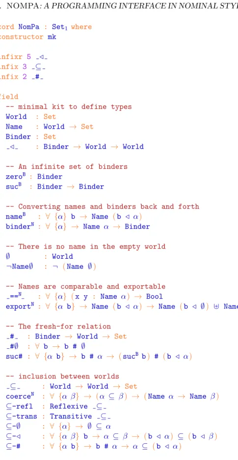
2.2 NomPa: A programming interface in nominal style . . . 48
2.2.1 All we need to define nominal syntax . . . 50
2.2.2 Building binders and names . . . 51
2.2.3 World widening: Name weakening . . . 53
2.2.4 Comparing and refining names . . . 56
3 Programming on top of NomPa 59 3.1 Various examples . . . 59
3.1.1 Example: computing free variables . . . 59
3.1.2 Example: working with environments . . . 60
3.1.3 Example: Term comparison . . . 62
3.2 Kits and Traversals . . . 63
3.2.1 Traversal Kits. . . 63
3.2.2 Coercing kit . . . 64
3.2.3 Renaming kits . . . 65
3.2.4 Substitution kit . . . 67
3.2.5 Other kits and combinators . . . 68
3.2.6 Reusable traversal . . . 68
3.2.7 Reusing the traversal. . . 69 9
3.2.8 Building any λ-term . . . 71
3.3 Towards elaborate uses of worlds . . . 72
3.3.1 Data type of “one hole contexts” . . . 72
3.3.2 Patterns a la ML . . . 73
3.3.3 Term and types: System F . . . 73
3.4 Advanced example: normalization by evaluation . . . 73
4 Behind the scene of the NomPa library 77 4.1 Implementation of NomPa . . . 77
4.2 Soundness: logical relations and parametricity. . . 80
4.2.1 Recap of the framework . . . 80
4.2.2 An example: Boolean values represented by numbers . 85 4.3 Relations for NomPa. . . 87
4.3.1 Relations for NomPa types . . . 88
4.3.2 NomPa values fit the relation . . . 91
4.3.3 An example not fitting the relation . . . 92
5 The de Bruijn approach 93 5.1 Introduction to de Bruijn indices . . . 93
5.1.1 bare: The original approach . . . 94
5.1.2 Maybe: The nested data type approach. . . 94
5.1.3 The Finapproach . . . 95
5.2 An interface for de Bruijn indices . . . 96
5.2.1 Singleton worlds! . . . 101
5.3 Examples and advanced operations . . . 101
5.3.1 Some convenience functions . . . 101
5.3.2 Building terms . . . 104
5.3.3 Computing free variables . . . 104
5.3.4 Generic traversal . . . 105
5.3.5 Nameless term comparison . . . 108
5.4 Logical Relations for de Bruijn indices . . . 109
5.4.1 Relations for the de Bruijn world operations. . . 109
5.4.2 De Bruijn functions fit the relation . . . 110
5.4.3 On the strength of free theorems . . . 111
5.4.4 Using logical relations and parametricity. . . 114
6 Variations and Related Work 119 6.1 Dynamically stratified representations . . . 120
6.1.1 Locally closed terms . . . 121
6.1.2 Building terms . . . 122
6.1.3 Performances . . . 123
6.1.4 Non-structural recursion . . . 124
6.1.5 Free atoms using openTm . . . 125
CONTENTS 11
6.1.7 Locally Nameless . . . 126
6.1.8 Locally Named . . . 128
6.1.9 When does this stratified technique pay off? . . . 130
6.2 de Bruijn levels . . . 133
6.2.1 Term comparison . . . 133
6.2.2 Kits and traversals . . . 134
6.2.3 Derived functions . . . 136
6.2.4 New inclusion rules . . . 137
6.2.5 Addition and subtraction kits . . . 137
6.2.6 Conversion with nominal terms . . . 138
6.3 Links: Binders as World Relations . . . 139
6.3.1 Terms and examples . . . 140
6.3.2 Implementations . . . 141
6.3.3 Building links and terms . . . 143
6.3.4 Kits and traversals . . . 144
6.4 Combining nominal and nameless styles . . . 148
6.5 Nominal types . . . 151
6.5.1 FreshML & Fresh OCaml types. . . 151
6.5.2 Cαml types . . . 159
6.5.3 Connection with Binders Unbound . . . 163
6.6 Related work . . . 167 7 Conclusion 175 7.1 Contributions . . . 175 7.2 Future work . . . 176 Bibliography 177 List of Figures 183 Index 185
Chapter 1
Introduction
Foreword
This document describes my work during these past three years which has been done under the direction of Fran¸cois Pottier. This work extends the research topic of safe meta-programming by pro-viding a novel approach to the representation of programs with names and binders. – Nicolas Pouillard
Safe meta-programming is a research topic which is part of the broader topic of programming language design. One of the goals of the research in programming language design is to provide programmers with better tools allowing to produce correct software applications in a reasonable amount of time. Since correct software applications (programs for short) are not supposed to crash, language designs have to incorporate safety features to detect programming errors as soon as possible. Modern language designs often come with some static disciplines such as lexical scoping, strong typing and the like. These static disciplines are used to reject the programs we do not want to run.
A program may process various forms of data such as numbers, text, spreadsheets, images, sound, and many more. Some programs process other programs, they are called meta-programs. Meta-programs cover a wide class of programs ranging from compilers, to static analyzers, code generators, etc. Proof systems, proof assistants and theorem provers are also meta-programs since propositions and proofs share the same kind of structure as programs. Moreover since language designs come with static disciplines, we claim that meta-programs should follow these disciplines when processing programs. For instance if a programAwritten in a programming languagePgenerates a programBwritten in a programming language Q, we want Ato follow the static discipline ofP, moreover we wantBwhich does not exist yet to follow the static discipline ofQ.
This first chapter aims at introducing all the notions to understand 13
the research problem that we are focusing on. This chapter requires lit-tle knowledge in the design of programming languages, but does require some knowledge about computers, mathematics and programming. Hence this introduction chapter can be safely skipped by readers accustomed with the research topic.
1.1
Programs and Programming Languages
To introduce the notions of programs and programming languages, let us start with an example of a simple program:
print "Hello! 2 times 21 is equal to " >> print (show (2 * 21) )
Most generally, programs are written to be executed on a computer. Running a program often results in the execution of different tasks and yields a final result. In our previous example the program is meant to print on the screen: “Hello! 2 times 21 is equal to 42”. Printing on the screen is done with the construct called print. This printing construct is used twice. The two uses are sequenced using the construct >>, which will perform the action on the left and then the action on the right. The number42is computed from the arithmetic expression2 * 21which is then turned into a printable form using the construct calledshow.
This program, such as any program, is written in a programming lan-guage. Programming languages are described by a finite set of constructs, rules explaining how the constructs can be used and rules giving the be-havior of programs. In our further examples the programming language contains constructs such as print, >>, show, *, character strings such as "Hello! 2 times 21 is equal to ", numbers such as 2 and 21, and parentheses. With these constructs our programming language is not much better than a simple calculator.
This tiny introductory programming language is built to be a subset of the Agda language. Agda [Norell, 2007] is a total functional program-ming language, based on dependent type theory. Agda is used thoroughly in this document. First it is used to introduce the research topic of meta-programming. Second it is used to implement our solution to the problem. Third it is used to formalize our system and show its soundness. Alas, ad-vanced languages such as Agda are far from simple to completely describe. The first set of programming constructs we introduce is roughly common to most languages and is described simply in great detail. The second set of constructs follows the development of functional programming languages (such as Haskell, ML, or Lisp). They are described more quickly and may require further reading about these topics. An excellent introduction
1.2. PROGRAM SYNTAX 15 to functional programming in Haskell is Graham Hutton’s “Programming in Haskell” [Hutton, 2007]. Moreover the third set of constructs is specific to dependently typed and total functional languages or even restricted to Agda only. To fully grasp these constructs we recommend further reading on these topics. In particular Ulf Norell’s [2007] PhD thesis on the theoret-ical and practtheoret-ical development of Agda is recommended.
1.2
Program syntax
Examples The following program makes use of the four basic arithmetic operators to compute the value42. Operators are attributed with their usual semantics, addition is + and multiplication is *. Subtraction and division (´ and ÷) are restricted to natural numbers, meaning that they return 0
when going out of range.
(1 + 1) * (28 ´ 14 ÷ 2)
The following program illustrates character string literals and their con-catenation with++. This program prints “Hello world!” on the screen: print ("Hello" ++ " " ++ "world!")
Our next program illustrates the use of show to turn a number into a character string containing its decimal representation. This program prints “show 1 renders as: 1” on the screen:
print ("show 1 renders as: " ++ show 1)
The following program illustrates the use of>> to sequence two actions from left to right. This program prints “Print me first.” and then prints “Then print me.” on the screen.
print "Print me first." >> print "Then print me."
We have lists in our programming language. The simplest list value is the empty list, written[]. The following program is a list with three elements, namely "a","bc" and "5":
[ "a" , "b" ++ "c" , show (2 + 3) ]
We go from lists to trees by using the construct called node. The first argument of node is the label of the node and the second is the list of children of the node. The following program represents a six-node tree
depicted hereafter: node "A"
[ node "B" []
, node "C" [ node "D" [] , node "E" [] ] , node "F" [] ]
A
B C
D E
F
Syntax of our arithmetic calculator The syntax of a programming language describes when a program has a valid “shape”. In particular it does not check if the program has a valid “meaning”. For instance, the program1 + "Hello!"has a valid syntax but no valid meaning in our tiny language.
Any non-empty sequence of digits (0,1,2,3,4,5,6,7,8,9) is a valid literal number and a valid program as well. A valid literal character string is a sequence of characters different from the double quote character (’"’) and surrounded by two double quote characters (we avoid talking about escape sequences because we do not need them here). If two programsp1andp2 are
syntactically valid, then for any operator • among +, ´,*, ÷,++,>> the programp1 • p2 is syntactically valid. These operators are said to be infix ,
meaning that they appear between the two operands. Ifpis a syntactically valid program, thenprint p,show pand (p)are syntactically valid. If p1,
p2, ..., pn are syntactically valid programs, then [ p1 , p2 , . . . , pn ]
is syntactically valid. Finally if p1 and p2 are syntactically valid programs
thennode p1 p2 is syntactically valid.
Of course not every textual program is syntactically valid. Consider this example: 3 + * 4. This program does not follow the rules we just described, hence it is rejected as syntactically invalid.
Syntax also comprises some details about layout and comments. Spaces and newlines are important to some extent. Spaces or parentheses have to be used to separate the words in a program. However, as long as they are separated, how many spaces or newlines are used to separate two words does not matter. There is special support in the syntax to embed comments in our programs. There are two syntaxes used in our language. A comment can start with {- and stop with -} or can start with -- and stop at the
1.3. TYPING 17 end of line. Here is a syntactically valid program to illustrate layout and comments:
print "Hello. . ." >> -- this prints Hello. . .
print {- extra spaces and comments are ok -} ". . . world!"
1.3
Typing
Typing captures, ahead of time, programs that may go wrong. Typing might be seen as a vigilant companion giving advice on our programs. When typing says that our program is ill-typed, then this is a program we may not want to even try running. If the typing says our program is fine, then we know for sure that the program will not crash.
Such a technology is to be applied systematically before running a pro-gram. It is an affordable safety measure which massively helps program development, maintenance, testing, and verification.
However, verifying that a program cannot crash without running it is a difficult problem to say the least. In particular we want the typing part of our system to always terminate, even if the given program does not terminate. We not only want the typing to terminate but to answer if the program is well-typed or not. If so we say that such a type system is decidable.
A type system is said to be sound if and only if every well-typed program is a non-crashing program. We expect every well-designed type system to be sound.
A type system is said to be complete if and only if every non-crashing program is well-typed. The decidability constraint entails that a type system will never be complete for non-trivial languages. For further reading on the topic of type systems we recommend reading “Types and Programming Languages” [Pierce,2002] and “Advanced Topics in Types and Programming Languages” [Pierce,2005].
Typing our arithmetic language The first goal of type systems is to prevent us from running programs that may crash. To do so, they define types, an abstraction to classify pieces of data. By extension, types also classify programs computing pieces of data. Types help to define a common “contract” for producers and consumers of a piece of data. This kind of “contracts” in on the shape of data. The more shapes are allowed by a type, the weaker the type is. The strength of a type affects producers and consumers in different ways. If a type is weak, it is easy for producers of this type to be well-typed. If a type is strong, the producers have to meet all the constraints imposed by the type. This is the opposite for consumers. If a type is strong, the data has a known precise shape, and the consumer
has an easy job. If a type is weak, then the consumer has to consider all the shapes that the data can take.
To illustrate the notion of typing, we equip our little programming lan-guage with such a type discipline. Step by step we introduce new types and how the constructs of our language are typed.
We have only a few types of values. We introduce the type N as the type of numbers (0, 1, 2, . . .) and of programs computing numbers (such as2 * 21).
Given a typeτ (such asN) and a programp(such as6 * 7), we writep has type τ to formally assert that the program p is of type τ. We call these type assertions typing judgements. The following paragraphs define the type system for our tiny language by giving a typing judgement for each construct.
For each numbern,nhas typeN. Given two programsp1andp2, if both
have type N, then p1 + p2, p1 * p2, p1 ´ p2, and p1 ÷ p2 all have type
Nas well. For instance with these rules one can formally assert: 6 * 7has typeN.
Our second type of basic values is text values. To this end we introduce the typeStringas the type of text values such as"Hello!"and of programs computing text values such as "Hello " ++ show 42. More precisely for each syntactically valid text values,shas typeString. If two programsp1
and p2 have type String then the program p1 ++ p2 has type String as
well. If a programphas typeNthenshow phas typeString.
It is now time to show an ill-typed program: "Hello!" ++ 42. While this program is syntactically valid, it does not follow our typing rules. There is indeed only one rule about the construct++. This rule imposes programs on each side of++to be of typeString. While"Hello!"is of typeString,
42 is not. The only rule that applies to42 says that it is of type N. Since StringandN are different, this program is rejected as being ill-typed.
Our little programming language has list values. However there is no single type for all lists. The type of a list depends on the type of its elements. We require all the elements of a list to have the same type. Given any typeA, ifp1,p2, ...,pn are programs of type Athen [ p1 , p2 , . . . , pn ] is of
type List A. Thus there is no single type for lists, but for each type A there is a type for lists where elements are of type A, namely List A. For instance [ 1 , 2 ] has type List N, and [ [ 1 , 2 ] , [ 3 ] ] has typeList (List N).
Our next type is the type of trees. Like for lists, the type of trees is parameterized by the type of its elements, namely the labels of nodes. For each type A, Tree A is the type of trees with labels of type A. To build a tree we use the constructnode: given a typeA, ifp1 has type Aand p2 has
typeList (Tree A) thennode p1 p2 has typeTree A.
1.4. PROGRAM REPRESENTATION, META-PROGRAMMING 19 node "A" [ node "B" [] , node "C" [] ]
This one has type Tree N:
node 1 [ node 2 [] , node 3 [] ]
This one is ill-typed, though:
node 1 [ node "B" [] , node "C" [] ]
Finally the type Interactive is used for programs interacting with the environment. We currently introduced only two forms of interaction, namely print and >>. Given a program p of type String, print p has type Interactive. This interactive program computes an interactive value which is meant to be triggered. Once the interactive value is triggered it prints the value of the textpon the screen.
The second form of interaction enables to sequence two interactive values. Given two programsp1 andp2 of typeInteractivethe programp1 >> p2
has typeInteractiveas well.
1.4
Program representation, meta-programming
When reading, writing, and editing programs we often work with the textual form of programs. We write programs in text files and so their representation is a sequence of characters in a file.Machines do not directly accept this kind of program for execution. Even languages very close to the hardware such as assembly languages are not directly understood by the machine. Hence programs are processed by other programs. These programs processing other programs are called meta-programs and are described in greater detail in the following section.
Up to here our simple programming language can process numbers, text, lists, trees and interactive values. What about programs? What is required to process programs themselves? If a program is simply a text in a file then our text value can represent programs. Here are two programs, the second is the textual representation of the first:
2 * (10 + 11) {- this should compute 42 -}
"2 * ( 10 + 11 ) {- this should compute 42 -}"
This is common knowledge nowadays that the textual representation is not adapted for any non-trivial processing. A first step called lexing gets rid of the lexical issues of layout and comments. The lexing step turns
the program text to a list of words, called tokens. These tokens are often annotated by a token class to distinguish numbers, operators, constructs. . . Here is the same program as a simple list of tokens:
[ "2" , "*" , "( " , "10" , "+" , "11" , " )" ]
This representation is still unworkable for non-trivial processing. In par-ticular there is too little structure in a list to reflect the program structure. To solve this issue, syntax trees have been introduced. Here is our same program, graphically depicted as a tree:
* num 2 + num 10 num 11
We picked names for some constructs such as “num” for numbers, “text” for text values, and “list” for lists. An exception is made for parentheses which no longer add any useful information and hence are not represented in the tree.
The process of translating text or tokens into a tree is called parsing. We will not discuss it more.
These syntax trees are generally called Abstract Syntax Trees or AST for short. Syntax trees are often said “abstract” because they no longer depend on some details of the “concrete” syntax.
Happily we have enough constructs in our language to build trees. We can hence show another representation of the same program as a tree built in our language:
node "*"
[ node "num" [ node "2" [] ] , node "+"
[ node "num" [ node "10" [] ] , node "num" [ node "11" [] ] ] ]
Representing programs of our language as values of our language itself is good to have but not necessary. However we can expect a programming language good at processing programs to be good at representing as many programs as possible.
1.4. PROGRAM REPRESENTATION, META-PROGRAMMING 21 How to choose the tree representation for a programming lan-guage? Here we made a simple choice: for each syntax rule we have a corresponding tree node labeled by the construct and with as many children as needed.
print "Hello! 2 times 21 is equal to " >> print (show (2 * 21) )
The syntax tree, graphically:
>>
text
Hello! 2 times 21 is equal to
print show * num 2 num 21
The syntax tree as a program: node ">>"
[ node "print"
[ node "text"
[ node "Hello! 2 times 21 is equal to " [] ] ] , node "print"
[ node "show"
[ node "*"
[ node "num" [ node "2" [] ]
An example to illustrate lists:
[ "a" , "b" ++ "c" , show (2 + 3) ]
The syntax tree, graphically:
list text a ++ text b text c show + num 2 num 3
The syntax tree as a program: node "list"
[ node "text" [ node "a" [] ] , node "++"
[ node "text" [ node "b" [] ] , node "text" [ node "c" [] ] ] , node "show"
[ node "+"
[ node "num" [ node "2" [] ]
1.5. NAMES AND LOCAL BINDINGS 23 An example to illustrate trees:
node "A" [ node "B" [] , node "C" [] ]
The syntax tree, graphically:
node text A list node text B list node text C list
The syntax tree as a program: node "node"
[ node "text" [ node "A" [] ] , node "list"
[ node "node"
[ node "text" [ node "B" [] ] , node "list" [] ] , node "node"
[ node "text" [ node "C" [] ] , node "list" [] ] ] ]
Meta-programming The broad topic of “programs processing other pro-grams” is called meta-programming. Sometimes meta-programming is given narrower definitions, but we find this one to better account for the different parts of the research field. Meta-programming comprises the generation, analysis, transformation of programs or similar objects such as formulae and proofs. Some programming languages are completely designed around meta-programming to support run-time code generation (MetaML [Taha,
1999], ‘C [Engler et al.,1996]). Program translations and optimizations, as done by compilers, are prime examples of meta-programming
1.5
Names and local bindings
Our programming language, while capable of arithmetic computations, in-teractions, and program representation, lacks the concept of names. We
hence introduce a construct to give a name to part of a program and refer to this part using the name. This enables an important goal of re-usability. In a program we should avoid to repeat ourselves. Hence if two parts are the same they may benefit from being written only once. Maybe more impor-tantly, changes to this part of the software logic, during later evolution of the code, only have to be done in one place instead of being duplicated. The syntax of this new construct relies on three keywordslet,=and in. If two programsp1 andp2 are syntactically valid andxis a name thenlet x =p1
in p2 is syntactically valid. Moreover, names (such asx) are valid program
themselves. If we want to print the same text twice we can write:
let x = print "Hello!" in
x >> x
If we replace the occurrences ofxby its definition (hereprint "Hello!") we obtain a program with the same behavior:
print "Hello!" >> print "Hello!"
The gain brought by sharing is significant. To illustrate this fact, we build an artificial example where each added let would double the size of the program if we could not uselet. Albeit artificial this example conveys the fact that sharing makes a big difference. The following example has 54 syntax nodes while the expanded version has 220 syntax nodes (only 124 if we reduce x0 to 0 first). Note also that the small computation done in x0
can be performed only once instead of 16 times.
let x0 = 42 ´ 2 * 21 in let x1 = node x0 [] in let x2 = node 1 [ x1 , x1 ] in let x3 = node 2 [ x2 , x2 ] in let x4 = node 3 [ x3 , x3 ] in node 4 [ x4 , x4 ]
1.6. SCOPING 25 node 4
[ node 3
[ node 2
[ node 1 [ node 0 [] , node 0 [] ] , node 1 [ node 0 [] , node 0 [] ] ] , node 2
[ node 1 [ node 0 [] , node 0 [] ] , node 1 [ node 0 [] , node 0 [] ] ] ] , node 3
[ node 2
[ node 1 [ node 0 [] , node 0 [] ] , node 1 [ node 0 [] , node 0 [] ] ] , node 2
[ node 1 [ node 0 [] , node 0 [] ]
, node 1 [ node 0 [] , node 0 [] ] ] ] ]
1.6
Scoping
A crucial aspect of the let construct is the scope of the newly introduced name. Given a namex and two programsp1 and p2, the programlet x =
p1 in p2 definesxto bep1 inp2. Thus, this makesxavailable inp2. We say
that the scope of the namex is the program p2. We also say that x scopes
overp2.
What should we do when a program uses a name that has not been defined? This is obviously an error and so should be detected as soon as possible. Here is an example to illustrate this kind of errors:
print x >> -- x is not defined, hence this is an error
let x = x in -- x is not yet defined
print x -- here x is defined
One may wonder if the same name could be used more than once. The scoping discipline we use allows this. In particular if one reuses a name already defined to define something else the new definition hides the previous one. Here is a correct program to illustrate the various scoping subtle cases:
let x = "1" in
print x >> -- this prints 1
let x = "2" in
print x >> -- this prints 2
print ( let x = "3" in x) >> -- this prints 3
( let x = "4" in print x) >> -- this prints 4
print x >> -- this prints 2 again
let x = x ++ x in
print x >> -- this prints 22
let x = let x = "5" in x ++ x in
print x -- this prints 55
We now introduce some vocabulary about names. In the program let
x = p1in p2, the namexis said to be bound . In particular it is bound inp2.
We call the namexin this position a binder . In the program print x, the namexis said to be free. We also call it an occurrence of x.
Sometimes names are also called variables. We try to prefer the term name over variable in this document. More precisely we use the term vari-able to represent the construct which holds just a name. For instance the programx + x contains two variables but only one name.
A program without any free names/variables is said to be closed. The set of free names can be defined inductively as follows. The set of free names of a variable x is the singleton set with the name x. The free names of an operation such as print p or show p are the free names of p. The free names of an operation such as p1 + p2 are the union of free names of p1
and ofp2. Finally the free names of let x = p1 in p2 are the free names
ofp2 minus x, union the free names of p1.
A name x is said to be fresh for a program p if the name x is not a member of the free variables of p. For example the name yis fresh for the programlet y =42in x + y, but the name xis not.
Two programs p1 and p2 are said to be α-equivalent if they differ only
by a consistent renaming of the bound names. Note that this is not a formal description of α-equivalence, but an informal definition appealing to our intuition of “name irrelevance”. Defining this relation precisely is one of the important part of this thesis. For instance the programs let x=21
in x + xandlet y=21in y + yare α-equivalent. The name of a variable should not have any importance except being a tool to reference a position in the program without ambiguities. α-equivalence is an equivalence relation. This means that the relation is reflexive (every program is α-equivalent to itself), symmetric (ifp1 is α-equivalent top2, thenp2 is α-equivalent top1),
and transitive (ifp1is α-equivalent top2 andp2is α-equivalent top3 thenp1
is α-equivalent top3). The α-equivalence is also a congruence, meaning that
ifp1 is α-equivalent top2 then if we put the programs in the context C[ ]
1.6. SCOPING 27 Typing our let construct We have introduced local definitions and variables and we now extend our typing discipline to these constructs. Like we have done for the previous constructs, we give the typing informally using a textual description. The program let x = p1 in p2 has type σ if
and only ifp1 has some type τ and thatp2 has typeσ assuming thatxhas
typeτ. To type a variable we use the assumptions we gathered so far. There are several ways to precisely describe how to manage these assumptions, but we do not detail them in this introduction.
Let us try to check the typing with an example. We check that the pro-gramlet x = 42in let y = show xin print yhas typeInteractive. To do so we first check that42has typeNwhich is true, then we must check that let y = show xin print y has type Interactive assuming thatx has type N. To do so we first check that show x has type String, which given the rule forshowamounts to check thatxhas typeN, which is true by assumption. We then check that print yhas type Interactiveassuming that y has type String. Given the rule for print this amounts to check thatyhas typeStringwhich is true by assumption.
Meta-programming and representation of variables How do we rep-resent variables and the let construct? It is reasonable to start with names being values of type String, each variable being a tree node that we call var, and the let construct being a node with three subtrees. The programlet x = 6in let y = x + 1in x * ycan thus be depicted as:
let x num 6 let y + var x num 1 * var x var y
This first approach is the root of the nominal approach that we describe in greater detail in chapter 2.
A different approach is to use de Bruijn indices [de Bruijn, 1972]. This representation is said to be nameless because variables are no longer iden-tified by a name but a notion of “distance” to the binding point. This nameless approach solves part of the problem by providing a canonical rep-resentation. However a major issue with this nameless representation is its
arithmetic flavor. Indeed properties about names and binders are turned into arithmetic formulae. This second approach is covered in chapter 5. Here is the same example using the de Bruijn style:
let num 6 let + var 0 num 1 * var 1 var 0
1.7
Empowering our language
Declarations and definitions We now fast-forward from our tiny subset of Agda to Agda itself as we need it in the remainder of this document. We start with declarations, which allow us to declare a symbol that can be used globally. This generally differs from theletconstruct whose scope is local. Moreover the declaration just specifies the type of the symbol. Subsequent phrases have to define this declared symbol. The declarations make use of the character: to separate the declared symbol from its type. The following line is read “Dear Agda, let us declarehello-worldof typeInteractive”: hello-world : Interactive
After the declaration must come the definition. The name of the defined symbol is recalled and a program is given for its definition:
hello-world = print "Hello World!"
Functions We introduce a new sort of types, namely function types. If σ andτ are types thenσ → τ is a type as well. This type represents functions whose domain is σ and co-domain is τ. Happily Agda functions are like mathematical functions and no surprise whatsoever will trouble this. The syntax for definitions enables the definitions of functions in a very simple way: we just give a name to the argument before the equal sign. To apply a
1.7. EMPOWERING OUR LANGUAGE 29 user defined function fto an argument x, the syntax is the lightest syntax possible:f x.
double : N → N double n = n + n
-- This program prints: 42
prog1 : Interactive
prog1 = print (show (double 21) )
The name n before the equal sign is a binder and scopes over the sub-program found after the equal sign. The scoping works pretty much like with thelet construct. Here is another example:
hello : String → Interactive
hello s = print ("Hello " ++ s ++ "!")
-- This program prints: Hello Functional World!
prog2 : Interactive
prog2 = hello "Functional World"
In order to receive multiple arguments one simply has to make functions return functions. Indeed the typeN → (N → N) is the type of a function taking a first number argument and returning a function taking a second number argument to finally deliver its result number. This is a pattern so common that we make the arrow type associate on right such that we can write the type this way: N → N → N. The same shortcut goes for function applications. Instead of writing (f x) y or worse (f(x))(y) we simply make the application associate on left, thus we can write f x y. Here is an example:
hello2 : String → N → Interactive
hello2 s n = print ("Hello " ++ s ++ " " ++ show n ++ "!")
-- This program prints: Hello World 42!
prog3 : Interactive
prog3 = hello2 "World" (2 * 21)
Data-types Among the types presented so far, N, List, Tree are user-defined in Agda. The general mechanism used to define these types is called inductive families. Inductive families generalize various forms of definition mechanisms such as sum and product types, regular tree types, algebraic
data types, and GADT s (generalized algebraic data-types). To define an inductive family, we need to declare its name and type, and declare as many data constructors as we want. Each data constructor has a name and a type as well. Let us study the definition for Bool, one of the simplest data type possible:
data Bool : Set where
false : Bool true : Bool
The first line declares Bool to have type Set. Indeed Set is a special type which is the type of basic types. Agda treats types like other values of the language. Then we define two data constructors calledfalseand true. These two constructors are the two only values of typeBool.
We now focus on the type of natural numbers, namelyN:
data N : Set where zero : N
suc : N → N
The first line declares N to have type Set. Then we define two data constructors called zero and suc. The constructor zero is introduced as a value of type N to represent the number 0. The constructor suc (for successor) is introduced as a function fromNtoN which might seem like a surprising beast. Two points are striking. First we are using the typeN in its own definition: this type is said to be recursive. The second point is to declare a function without giving it a definition. Indeedsuc has no other definition, and thus giving it an argument does not trigger a computation. For instancesuc zerostays stuck like that and does not reduce further. The language is built to take advantage of data constructors to define functions by pattern matching.
Note that the same name can be used for different data constructors of distinct data types. Agda makes use of type annotations to resolve ambiguities.
To illustrate definitions made with pattern matching the following pro-gram defines a function callednot which negates a Boolean value:
not : Bool → Bool not true = false not false = true
This definition is made of two equations: one for each constructor of the inspected argument. In the case for true we return false and in the case forfalsewe returntrue.
1.7. EMPOWERING OUR LANGUAGE 31 We now go on a more interesting definition made with pattern matching. The following program defines a function calledtriplewhich multiplies by three its argument:
triple : N → N
-- 3 * 0 = 0
triple zero = zero
-- 3 * ( 1 + n ) = 3 + 3 * n
triple (suc n) = suc (suc (suc (triple n) ) )
While this definition is longer than we could expect (triple n = 3 * n), it has a pedagogical interest. This definition is made of two equations: one for each constructor of the inspected argument. In the successor case the function tripleis used in the definition of tripleitself! This function is said to be recursive.
We can now reveal that all the operations on natural numbers we have seen so far are actually defined within the language using recursive defini-tions. Here are for instance the definitions for+and *. To express that we want these operators to be infix, we declare+as +. Each indicates special places where operands should go. Both functions + and * pattern-match on their first argument:
+ : N → N → N zero + n = n -- 0 + n = n suc m + n = suc (m + n) -- ( 1 + m ) + n = 1 + ( m + n ) * : N → N → N zero * n = zero -- 0 * n = 0 suc m * n = n + m * n -- ( 1 + m ) * n = n + m * n
The notation we used for literal numbers such as2or4is actually strictly equivalent tosuc (suc zero)andsuc (suc(suc (suc zero)))respectively. We define a last operation on natural numbers, namely division by two. We do not show the definition for÷. Indeed, division by a known constant is indeed much simpler to define recursively and illustrates subtler pattern matching. The function is declared as /2 and hence has to be used either prefix as /2 4or postfix as 4 /2. You can notice how spaces are of prime importance in Agda since they allow to freely choose meaningful names for functions. The function /2proceeds as follows. The two base cases for zero and one are handled in the first two equations. The last equation deals with all numbers strictly greater than one which makes a simple recursive call to
obtain our result: /2 : N → N
-- 0 / 2 = 0
zero /2 = zero
-- 1 / 2 = 0
suc zero /2 = zero
-- ( 2 + n ) / 2 = 1 + n / 2
suc (suc n) /2 = suc (n /2)
Polymorphism Sometimes functions do not need to know the nature of parts of their arguments. This means that many types could be accept-able for such functions. An extreme case is the identity function which simply returns its argument. What type should we give it? N → N, String → String, or List N → List Nand the list goes on indefinitely. The solution to this issue is called polymorphism. We generalize the type of the function type to∀{A} → A → A, which reads “for all typeAa function fromAtoA”. The polymorphic identity function (id) can thus be written: id : ∀{A} → A → A
id x = x
-- The function id can be used at different types
prog4 : Interactive
prog4 = print (id "Hello " ++ show (id 42) )
Lists We define two new data types that we assumed to be special so far, namely List and Tree. The type for lists –such as the type N– is made of two data constructors. A base constructor named[] and pronounced “nil” represents the empty list. Another constructor named :: and pronounced “cons” appends one element to the front of a list. The notation [ n1 ,
n2 , . . . ] is simply a shorthand for the less familiar n1 :: n2 . . . :: [].
data List (A : Set ) : Set where
[] : List A
:: : A → List A → List A
1.7. EMPOWERING OUR LANGUAGE 33 show one of them which while being simple can be insightful. The func-tion length takes a list and returns its length as a natural number. The function is defined with two equations: one for the empty list whose length is zero, and one for any constructed list whose length is the successor of the length of the tail of the list. In short this function replaces the lists constructors by the constructors of natural numbers. This highlights the fact that both types share the same structures. Natural numbers are lists of meaningless elements and lists are natural numbers whose constructors are annotated by elements. The functionlengthis polymorphic. It takes a list, forgets the elements to reveal the bare structure behind any list: a natural number.
length : ∀{A} → List A → N
length [] = zero
length (x :: xs) = suc (length xs)
Let us remark that since we make no use of the name x in the second equation for length we could have use the special wildcard pattern. The wildcard pattern is noted and is used to replace a name to state that we do not use this part of the value.
Another common function on lists is the functionmap. The functionmap takes a function f from a type A to a type B, and also takes a list of type List A on which it applies f on every element to build the result-ing list of typeList B. Sincemaptakes a function as argument it is what we call an higher-order function. Moreover, the function map is also recursive and polymorphic. Here is the definition ofmap:
map : {A B : Set} → (A → B) → List A → List B map f [] = []
map f (x :: xs) = f x :: map f xs
We now introduce an extension to pattern matching equations, namely thewith construct. This construct extends a pattern-matching-based defi-nition with new columns. This construct is of great effect when combined with dependent pattern-matching. However, we present it here on a simpler example, the function to filter a lists. The function filter, takes a pred-icate p and a list xs and keeps only the elements of xs which statisfy the predicate p. The with construct is used here to select a branch according to the result of the predicate:
filter : {A : Set} → (A → Bool) → List A → List A filter p [] = []
filter p (x :: xs) with p x
filter p (x :: xs) | true = x :: filter p xs filter p (x :: xs) | false = filter p xs
Moreover, an ellipsis ... can be used to elide a redundant equation prefix. Hence we can write filter, this way:
filter : {A : Set} → (A → Bool) → List A → List A filter p [] = []
filter p (x :: xs) with p x
... | true = x :: filter p xs
... | false = filter p xs
Trees and forests We continue with trees the exploration of our pre-viously assumed basic types. Trees can be defined with a new data type. This data type Tree has a single data constructor named node with two arguments: the node label of type A and the children as a list of subtrees (List (Tree A)).
data Tree (A : Set ) : Set where
node : A → List (Tree A) → Tree A
Commonly we call forests the lists of trees. The name is suggestive and the type is shorter to write. Its definition shows how types are treated such as other values:
Forest : Set → Set
Forest A = List (Tree A)
Trees and forests are interdependent. They finally build a pair of mu-tually recursive types. This is the occasion to define a pair of mumu-tually recursive functions. We definesumTree and sumForest which respectively compute the sum of the labels in a tree of natural numbers and in a forest of natural numbers. For Agda to accept these definitions, the two declarations must come before the two definitions.
1.7. EMPOWERING OUR LANGUAGE 35 sumForest : Forest N → N
sumTree (node n forest) = n + sumForest forest
sumForest [] = 0
sumForest (tree :: forest) = sumTree tree + sumForest forest
Robust program representations So far we have seen three distinct types to represent programs: text values (String), lists of tokens (List String), and trees (Tree String). These three types are based on the type String and thus they are loose representations. For instance the tokens can be malformed tokens and the tree labels could be malformed as well. We could introduce data types for tokens and tree labels which rule out the malformed text values. However we can do even better. Here is a data type for our tiny programming language of the beginning:
data Program : Set where
‘num : N → Program ‘text : String → Program
‘list : List Program → Program
‘node : Program → Program → Program ‘+ : Program → Program → Program ‘´ : Program → Program → Program ‘* : Program → Program → Program ‘÷ : Program → Program → Program ‘++ : Program → Program → Program ‘print : Program → Program
‘show : Program → Program
‘>> : Program → Program → Program ‘var : String → Program
‘let : String → Program → Program → Program
The type Program is a recursive type inducing a specialized tree struc-ture. Each construct is modeled by a single data constructor which is named with the corresponding label we have for trees plus an extra‘character. The data constructor also specifies how many subtrees are expected and what kind of subtree is expected. Here are two of our previous examples repre-sented with our type Program:
prog4 : Program
prog5 : Program
prog5 = ‘>>
(‘print (‘text "Hello! 2 times 21 is equal to ") ) (‘print (‘show (‘* (‘num 2) (‘num 21) ) ) )
Here are now a few programs that cannot be represented with the data type Program. Indeed while all correct programs can be represented, this simple data type already rules out plenty of wrong programs. Here is first a list of syntactically wrong programs represented as texts:
[ "2 *" -- missing operand
, "( 2" -- missing parenthesis
, "2 {- " -- non-closed comment
, "bla" -- unknown construct or variable
]
Here is now a list of still syntactically wrong programs represented as trees:
[ node "+" [ p ] -- missing operand
, node "+" [ p1 , p2 , p3 ] -- extra operand
, node "bla" [] -- unknown construct
, node "var" [ node "bla" [] ] -- unknown variable
]
Finally, there are still wrong programs accepted by all of our representa-tions. Those are the ill-scoped programs and the ill-typed programs. Here is a list of ill-scoped or ill-typed programs using the typeProgram:
[ ‘var "bla" -- unknown variable
, ‘+ (‘num 1) (‘text "Hello!") -- ill-typed
, ‘let "x" (‘var "x") (‘num 1) -- unknown variable
]
The rest of this document focuses on how to improve program represen-tation to better account for the handling of variables in programs.
Declaring the last operations We have shown how various constructs of our tiny programming language can be defined in Agda. We now quickly declare the remaining constructs that can be Agda functions. Thus we declare ´, ÷ ,show, ++ ,print, and >> . While we give no definitions for these functions the declarations describe both their syntax and their
1.7. EMPOWERING OUR LANGUAGE 37 typing very concisely:
´ : N → N → N ÷ : N → N → N show : N → String
++ : String → String → String print : String → Interactive
>> : Interactive → Interactive → Interactive
The core constructs from our tiny language that we do not define are literals (numbers, texts, lists), variables and the let construct. However, in order to use all these functions and constructors we introduced a fairly-discrete construct, namely application. Since application is written as a simple juxtaposition (using spaces or parentheses) we might forget it. In our tree representation we use the label"app" for these application nodes. We can now view the example program2 * (10 + 11) as a tree where the application nodes replace the special nodes of operations:
app app * num 2 app app + num 10 num 11
Agda types In Agda, the usual function space is writtenA → B, while the dependent function space is written(x : A) →B or ∀ (x : A) → B. An implicit parameter, introduced via ∀{x : A} → B, can be omitted at a call site if its value can be inferred from the context. There are shortcuts for introducing multiple arguments at once or for omitting a type annotation, as in∀{A} {i j : A} x → e.
In Agda,Set(orSet0) is the type of small types such asN,List String, and Maybe (Bool × N). Set1 is the type of Set,Set → Bool,N → Set, and Set → Set.
There is no specific sort for propositions in Agda: everything is inSet ` for some `. The unit type is a record type with no fields named >. It also represents the True proposition. The empty type is named ⊥ and is an
(inductive) data type with no constructors. It also represents the False proposition. The negation¬ A is defined asA → ⊥.
Lexical conventions We recall that Agda is strict about whitespace: x≤yis an identifier, whereas x ≤ y is an application. This allows naming a variable after its type (deprived of any whitespace). For example: x≤y might be a variable of typex ≤ y, that is, a proof of x ≤ y.
Various notions of equality Advanced logics and proof systems exhibit various forms of equality. The definitional equality is a first form of equality which is deeply rooted in the computation rules of the programming lan-guage itself, here, Agda. Two terms are definitionally equal if and only if they can both reduce to a common term. In Agda, the reduction is a combination of β-reductions, η-conversions, and application of the definition equations.
Here are a few examples of definitionally equal terms. We informally use=for this equality since this symbol is the one used for definitions.
( λ x → x) suc zero = suc zero suc = λ x → suc x
zero + n = n
Here is an example of two terms which are not definitionally equal even if this equality seems natural:
n + zero 6= n
Definitional equality is completely automatic and thus requires no help from the user. However if we want to include some reasoning steps we can use the propositional equality. The symbol used in Agda and further in this document is ≡. To simplify matters, here is the definition of the proposi-tional equality specialized to values of small types (Set0), namely ≡0 :
data ≡0 {A : Set0} (x : A) : A → Set0 where
refl : x ≡0 x
ı0 : {A : Set0} → A → A → Set0
x ı0 y = ¬(x ≡0 y)
We do not intend to explain the subtleties of such a definition. We only mention that there is a single constructor for this type requiring both sides to be same, hence definitionally equal.
1.7. EMPOWERING OUR LANGUAGE 39
-- This is definitionally true, hence immediately proven by refl
zero + n ≡ n
-- This is provable by a simple induction on n
∀ n → n + zero ≡ n
Sometimes, two functionsfandgcannot be proved propositionally equal but still produce the same output on every possible input. In this case, the functions f and g are said to be equal pointwise. The symbol for point-wise equality is $. Here is the definition of pointwise equality in Agda, specialized to small types (Set0), non-dependent functions:
$0 : {A B : Set0} (f g : A → B) → Set0
f $0 g = ∀ x → f x ≡0 g x
To illustrate pointwise equality we define the functionnot2which iterates the functionnottwo times.
not2 : Bool → Bool not2 x = not (not x)
We then show that the function not2 is equal pointwise to the identity function. Given the definitions for $0 and not2 this exactly amounts to
show: ∀ x → not (not x) ≡ x. not2$id : not2 $0 id
not2$id true = refl -- true = not ( not true ) definitionally
not2$id false = refl -- false = not ( not false ) definitionally
Equalities are said to be either intensional or extensional. Let us use sorting functions as an example to illustrate the difference. If we have two different sorting functions each implementing one sorting algorithm such as bubble sort and quick sort. The two functions are said to be extensionally equal since they both return the same sorted list for any given list. However bubble sort and quick sort are not intentionally equal. The intention is actually opposite. When we write a quick sort function, we intentionally want to make it different than bubble sort!
In Agda both the definitional and the propositional equalities are cur-rently intensional. There is an ongoing will to make the propositional equal-ity more extensional. While this sounds like a radical change, the proposi-tional equality is actually already compatible with extensionality. Indeed, there is no way to contradict extensionality with the current propositional equality. In short there is no proof than quick sort is different from bubble sort and thus making them provably equal introduce no contradiction.
The pointwise equality is by construction extensional and in section 4.2
we explain a generalized definition to relate functions which sends related inputs to related outputs.
Full development online We use some definitions from Agda’s standard library: natural numbers, booleans, lists, and applicative functors (pure and f ).
For the sake of conciseness, the code fragments presented in this docu-ment are sometimes not perfectly self-contained. However, a complete Agda development is available online [Pouillard,2011a].
Outline This document is organized as follows.
The next three chapters delve into the nominal approach. We introduce the nominal approach (chapter 2) and present our system: a safe program-ming interface for the nominal style. We then present how to use it (chap-ter 3), and what happens behind the scene to implement it and show its safety (chapter4).
The next chapter (5) covers a nameless approach known as “de Bruijn indices”. We present how to seamlessly extend our system to this new approach. This chapter covers the same aspects: the interface and its im-plementation, its usage, its soundness.
The remaining chapter (6discusses different variations and combinations of these variations. At the same time this chapter covers the related work and concludes.
Chapter 2
The nominal approach
This chapter is organized as follows. The first section informally introduces and presents several techniques to represent data structures with bindings in a nominal style. Section2.2describes our solution, an interface to program with names and binders.
2.1
Introduction to the nominal approach
2.1.1 Warm-up: the bare nominal approach
The bare approach to abstract syntax with names and binders in nominal style requires very little infrastructure to start with. Names and binders are represented by so-called atoms. The set of atoms is countably infinite and the only required operation is an equality test. Using natural numbers as a concrete representation for atoms is a common and sensible choice.
-- A set of atoms ( could be N )
Atom : Set
-- Atom is countably infinite; here are some atoms: -- x,y,z... could be represented by 0,1,2...
x y z f g {-...-} : Atom
-- The equality test on atoms
==A : (x y : Atom) → Bool
Given the type Atom we can readily define algebraic data types for ab-stract syntax with names and binders. Our running example is the untyped λ-calculus defined below. The typeTmA (Tm for “term” andA for “atom”) is
made of three data constructors. The constructorVis for variables and sim-ply holds an atom. The constructor · is the function application construct made of two subterms. The constructor ň takes an atom and a subterm
in which this atom is considered bound. This means that the construct ň is introducing a variable. On contrary the atom in the construct V is said to be free. Indeed this atom is supposed to refer to a bound atom. The constructor Letalso takes an atom but two subterms. The atom is bound in the second subterm only.
data TmA : Set where
V : (x : Atom) → TmA · : (t u : TmA) → TmA
ň : (b : Atom) (t : TmA) → TmA Let : (b : Atom) (t u : TmA) → TmA
It is striking that there is no formal distinction between the atoms that represent binders and those that represent occurrences. Neither is there any indication of the scope of the binders. This calls for improvement.
We consider it very important to highlight that atoms are used for two distinct purposes whether they are in a binding position or a free position. Starting from section2.2, we embrace that distinction and provide distinct types for these usages.
Here are two term examples, the identity function and the application function: -- λx. x idTmA : TmA idTmA = ň x (V x) -- λf. λx. f x apTmA : TmA apTmA = ň f (ň x (V f · V x) )
The strength of this approach resides in its simplicity. The representation of terms closely follows the concrete syntax of the language. The main issue is adequacy: there are multiple equivalent representations of the “same” term.
Indeed the choice of atoms is fairly arbitrary. Two terms can represent the same piece of syntax when they differ only by a consistent renaming of bound names. In this situation two such terms are said to be α-equivalent. Here are for example two α-equivalent terms:
tx : TmA
tx = ň x (V f · V x)
ty : TmA
2.1. INTRODUCTION TO THE NOMINAL APPROACH 43 The termtx is α-equivalent to ty since consistently renaming the bound name x by y in the term tx yields the term ty. Respectively consistently renaming y by x in ty yieldstx. However α-equivalence can be subtle, let us observe a third termtf which is not α-equivalent to neither tx norty: tf : TmA
tf = ň f (V f · V f)
An inconsistent renaming of the bound namexbyfintxyieldstf, while a consistent renaming of the bound namefby xintf does not yield tx.
We do not delve more into the details of α-equivalence yet. We focus on the fact that the concrete naming of a term is a representation issue and should not be relevant for the computation. In particular, good functions should be independent of this representation issue. This property can be stated as follows:
A function is well-behaved if, when applied to α-equivalent arguments, it produces α-equivalent results.
To illustrate well-behaved functions we give a few examples. The fol-lowing functions rmA (removes an atom from a list) and fv (lists the free variables/atoms of a term) are well-behaved:
rmA : Atom → List Atom → List Atom rmA [] = []
rmA x (y :: ys) =
if x ==A y then rmA x ys else y :: rmA x ys
-- Since rmA behaves well, this holds:
test-rmA : rmA x [ x ] ≡ rmA y [ y ] test-rmA = refl -- both reduces to []
fv : TmA → List Atom fv (V x) = [ x ]
fv (t · u) = fv t ++ fv u fv (ň x t) = rmA x (fv t)
fv (Let x t u) = fv t ++ rmA x (fv u)
-- Since fv behaves well, this holds:
test-fv : fv tx ≡ fv ty
We now illustrate misbehaving functions with two examples. The func-tion ba computes the list of bound atoms. The function cmp-ba takes two terms and compare their bound variables if both areňconstructs.
ba : TmA → List Atom ba (ň x t) = x :: ba t ba (Let x t u) = x :: ba t :: ba u ba (t · u) = ba t ++ ba u ba (V ) = [] [x]ı[y] : [ x ] ı [ y ] [x]ı[y] = {! omitted !}
-- Since ba does not behave well:
test-ba : ba tx ı ba ty test-ba = [x]ı[y]
cmp-ba : TmA → TmA → Bool cmp-ba (ň x ) (ň y ) = x ==A y
cmp-ba = false
-- Since cmp-ba does not behave well:
test-cmp-ba : cmp-ba tx tx ı cmp-ba tx ty test-cmp-ba ( ) -- true ı false
In traditional informal developments, α-equivalence is identified with equality. The upside is that every definition respects α-equivalence. Hence functions automatically map α-equivalent inputs to α-equivalent outputs. The downside is that building functions is more difficult. Indeed what were misbehaving functions before, are not functions anymore when we identify α-equivalence and equality. They are not functions simply because they map equal inputs to different outputs.
One of the goals of our system is to guarantee that well-typed functions are well-behaved. A function likecmp-bais ill-typed in our system. A function like ba is typed differently than the function fv, effectively disarming the functionba.
2.1.2 Using well-formedness judgements
One way to define the scoping rules is to define a well-formedness judgement. It can be done using a recursive predicate over the structure of terms. It is a well-known technique used in the definition of type systems. The standard presentation makes use of a set of inference rules where judgements are