Evaluation of system-on-chip devices for embedded real-time simulators of electrical systems

HAL Id: tel-02284435

https://tel.archives-ouvertes.fr/tel-02284435

HAL is a multi-disciplinary open access archive for the deposit and dissemination of sci-entific research documents, whether they are pub-lished or not. The documents may come from teaching and research institutions in France or abroad, or from public or private research centers.

L’archive ouverte pluridisciplinaire HAL, est destinée au dépôt et à la diffusion de documents scientifiques de niveau recherche, publiés ou non, émanant des établissements d’enseignement et de recherche français ou étrangers, des laboratoires publics ou privés.

real-time simulators of electrical systems

Daniel Tormo Borreda

To cite this version:

Daniel Tormo Borreda. Evaluation of system-on-chip devices for embedded real-time simulators of electrical systems. Electronics. Université de Cergy Pontoise, 2018. English. �NNT : 2018CERG0969�. �tel-02284435�

E VA L U AT I O N O F S Y S T E M - O N - C H I P D E V I C E S F O R E M B E D D E D R E A L - T I M E S I M U L AT O R S O F E L E C T R I C A L S Y S T E M S

d a n i e l t o r m o b o r r e d à

A dissertation for becoming Doctor of Philosophy in Electrical and Electronic Engineering

Année 2018 Université Paris Seine

THÈSE

Présentée pour obtenir le grade de

DOCTEUR DE L’UNIVERSITÉ PARIS SEINE

École doctorale: Sciences et Ingénierie

Spécialité: Génie Électrique et Électronique

Soutenue publiquement le 11 Juillet 2018 par d a n i e l t o r m o b o r r e d à

E VA L U AT I O N O F S Y S T E M - O N - C H I P D E V I C E S F O R E M B E D D E D R E A L - T I M E S I M U L AT O R S O F E L E C T R I C A L S Y S T E M S

Laboratoire de Systèmes et Applications des Technologies de l’Information et de l’Énergie (SATIE) - CNRS UMR8029

Devant le Jury composé par

Président : Prof. Serge PIERFEDERICI Univ. de Lorraine

Rapporteurs : Prof. Guillaume GATEAU Univ. de Toulouse

Prof. Mickaël HILAIRET Univ. de Franche-Comté

Examinateur : Prof. Ramón BLASCO-GIMÉNEZ Univ. Politècnica de València

Directeur de Thèse : Prof. Eric MONMASSON Univ. Paris Seine

of Electrical Systems, A dissertation for becoming Doctor of Philosophy in Electrical and Elec-tronic Engineering, © 11th July 2018

Per als meus pares i germans. Per als meus nebots. Per a tots aquells que en major o menor mesura m’han ajudat a ser la persona que sóc. Esta tesi no haguera sigut possible sense tots

vosaltres.

A tots, gràcies de tot cor.

I recordeu: sigueu curiosos. La curiositat és la recerca constant de coneixement.

— D. Tormo

To my parents and brothers. To my niece and nephews. To all those who to a greater or lesser extent have helped me become the person I am. This thesis would not have been

possible without all of you. Thank you very much indeed.

And remember: be curious, because curiosity is the constant pursuit of knowledge.

A B S T R A C T

This Doctoral Thesis is a detailed study of how suitable System-on-Chip (SoC) devices are for implementing Embedded Real-Time Simulators (eRTS) of electromechanical and power elec-tronic systems. This emerging class of Real-Time Simulators (RTS) are not only expected for Hardware-in-the-Loop (HIL) validations of systems; but they also have to be embedded within the controller to play several roles like observers, parameter estimation, diagnostic, health monitoring, fault-tolerant and sensorless control, etc.

The design of these Intellectual Properties (IP) must rigorously consider a set of constraints at different development stages: (i) during the modeling of the system to be real-time simulated; (ii) during the digital realization of the IP; and also (iii) during its final implementation in the digital platform. Thus, the conducted work of this Thesis focuses specially on this last stage and its aim is to evaluate the time/resource performances of recent SoC devices and study how suitable they are for implementing eRTSs. These kind of digital platforms com-bine powerful general purpose processors, a Field-Programmable Gate Array (FPGA) and other peripherals which make them very convenient for controlling and monitoring a complete system.

One of the limitations of these devices is that control engineers are not particularly famil-iarized with FPGA programming, which needs extensive expertise in order to code these highly sophisticated algorithms using Hardware Description Languages (HDL). Notwithstand-ing, there exist High-Level Synthesis (HLS) tools which allow to program these devices using more generic programming languages such as C, C++ or SystemC. Moreover, by inserting directives and constraints to the source code, these tools can produce different hardware im-plementations (e.g. full-combinatorial design, pipelined design, parallel or factorized design, partition or arrange data for a better utilisation of memory resources, etc.).

This dissertation is based on the implementation of two representative applications that are well known in our laboratory: a Doubly-fed Induction Generator (DFIG) commonly used as wind turbines; and a Modular Multi-level Converter (MMC) that can be arranged in different configurations and utilized for many different energy conversion purposes. Since the DFIG has low/medium system dynamics (electrical and mechanical ones), both a full-software im-plementation using solely the ARM processor and a full-hardware imim-plementation using HLS to program the FPGA will be evaluated with different design optimizations and data formats (64/32-bit floating-point and 32-bit fixed-point). Moreover, it will also be investigated whether a system of these characteristics is interesting to be run as a hardware accelerator. Different data transfer options between the Processor System (PS) and the Programmable Logic (PL) have been studied as well for this matter. Conversely, because of its harsh dynamics (switching dynam-ics), the MMC will be implemented only with a full-hardware approach using HLS tools, as well.

For the experimental validation of this Thesis work, a complete MMC test bench has been built from scratch in order to compare the real-world results with its SoC eRTS implementa-tion.

Keywords – Embedded Real-Time Simulator, System-on-Chip, High-Level Synthesis, Modu-lar Multi-level Converter, Field-Programmable Gate Array

R É S U M É

L’objectif de ce travail de Thèse est d’évaluer les capacités de composants numérique de type Système-sur-Puce (SoC en anglais) pour l’implantation de Simulateurs Temps Réel Embar-qués (eRTS en anglais) de systèmes électromécaniques et d’électronique de puissance. En ef-fet, l’utilisation de ces simulateurs n’est pas seulement limitée aux validations matériel dans la boucle (en anglais Hardware-in-the-Loop ou HIL) du système mais doivent également être embarqués avec le contrôleur afin d’assurer plusieurs fonctionnalités additionnelles comme l’observation, l’estimation, commande sans capteur (ou sensorless), le diagnostic ou la surveil-lance de la santé, commande tolérante aux défauts, etc.

La réalisation de ces simulateurs doit néanmoins considérer plusieurs contraintes à plusieurs niveaux de développement : durant la modélisation de la partie du système à simuler en temps-réel, durant la réalisation numérique et enfin durant l’implantation sur le composant numérique utilisé. Ainsi, le travail réalisé durant cette Thèse s’est focalisé sur ce dernier niveau et l’objectif était d’évaluer les capacités temps/ressources des composants de type SoC pour l’implantation de modules eRTS. Ce type de plateformes intègrent dans un même com-posant de puissants processeurs, un circuit logique programmable (Field-Programmable Gate Array ou FPGA), et d’autres périphériques, ce qui offre plusieurs opportunités d’implantation. Afin de pallier les limitations liées au codage VHDL de la partie FPGA, il existe des out-ils High-Level Synthesis (HLS) qui permettent de programmer ces dispositifs en utilisant des langages à haut niveau d’abstraction comme C, C++ ou SystemC. De plus, en incluant des directives et contraintes au code source, ces outils peuvent produire des implémentations matérielles différentes (architecture totalement combinatoire, « pipeline », architecture paral-lélisées ou factorisées, arranger les données et leurs formats pour une meilleure utilisation des ressources de mémoire, etc.).

Dans le but d’évaluer ces différentes implantations, deux cas d’études ont été choisis : le premier se compose d’un Générateur Asynchrone à Double Alimentation (GADA) et le second d’un Convertisseur Modulaire Multiniveau (ou Modular Multi-level Converter - MMC). Vu que la GADA a une dynamique basse/moyenne (dynamiques électriques et mécaniques), deux versions d’implantations ont été évaluées : (i) une implantation full-software en utilisant seule-ment les processeurs ARM; et (ii) une implantation full-hardware en utilisant l’outil HLS pour programmer la partie FPGA. Ces deux versions ont été évaluées avec différentes optimisa-tions du compilateur et trois formats de données: 64/32-bit en virgule flottante, et 32-bit en virgule flottante. L’approche mixe software/hardware a également été évaluée à travers la carac-térisation des transferts de données entre le processeur et l’IP eRTS implantée dans la partie FPGA. Quant au convertisseur MMC, sa complexité et sa forte dynamique (dynamique de commutation) impose une implantation exclusivement full-hardware. Celle-ci a également été réalisée à base d’outils HLS.

Enfin pour la validation expérimentale de ce travail de Thèse, une maquette à base de convertisseur MMC a été construite dans le but de comparer des mesures du système réel avec les résultats fournis par l’IP eRTS.

Mots clés – Simulateurs en temps réel embarqués, Système-sur-puce, Synthèse de haut niveau, Convertisseur Modulaire Multiniveaux, Field-Programmable Gate Array

R E S U M

L’objectiu d’aquest treball de Tesi és avaluar les capacitats de dispositius digitals de tipus System-on-Chip (SoC) per a la implantació de Simuladors en Temps Real Embarcats (Embedded Real-Time Simulators o eRTS en anglès) de sistemes electromecànics i d’electrònica de potèn-cia. Aquesta classe emergent de Simuladors en Temps Real (RTS) no estan pensats només per a realitzar validacions de controladors amb Hardware-in-the-Loop (HIL); aquests deuen estar em-barcats amb el controlador per a executar diferents tasques tals com observadors, estimació de paràmetres, diagnòstic, monitorització de l’estat de salut del sistema, control amb tolerància a fallades o sensorless, etc.

El disseny d’aquestes Propietats Intel·lectuals (IP) deu considerar rigorosament certes restric-cions en cadascuna de les etapes de desenvolupament: (i) durant el modelat del sistema a ser simulat en temps real; (ii) durant la discretització de l’IP; i també (iii) durant la fase final d’implementació en la plataforma digital escollida. Per això, el present treball s’enfoca especí-ficament en aquesta última etapa i el seu objectiu és avaluar el rendiment considerant temps d’execució i recursos utilitzats dels dispositius SoC i estudiar quant apropiats són per a im-plementar eRTSs. Aquests tipus de plataformes combinen potents processadors de propòsit general, Field-Programmable Gate Arrays (FPGA), juntament amb altres perifèrics que els fan molt adequats per a controlar i monitoritzar un sistema complet.

Una de les limitacions d’aquests dispositius és que els enginyers de control no estan partic-ularment familiaritzats amb la programació d’FPGAs, els quals requereixen una gran exper-iència per a programar els algoritmes altament sofisticats utilitzant Llenguatges de Descripció Hardware (HDL). No obstant això, existixen ferramentes de Síntesi d’Alt Nivell (High-Level Synthesis en anglès o HLS) que permeten programar aquests dispositius utilitzant llenguatges de programació més genèrics tals com C, C++ o SystemC. A més a més, inserint directives i restriccions al codi font, aquestes ferramentes poden produir diferents implementacions hard-ware (e.g. disseny completament combinacional, disseny segmentat, disseny paral·lel o fac-toritzat, partint o reordenant les dades per a una millor utilització dels recursos de memòria, etc.).

Aquesta dissertació està basada en la implementació de dos aplicacions representatives que són ben conegudes al nostre laboratori: un Generador Inductiu Doblement Alimentat (Doubly-fed Induction Generator en anglès o DFIG) utilitzat normalment en turbines eòliques; i un Con-vertidor Modular Multinivell (Modular Multi-level Converter o MMC) que pot ser assemblat en diferents configuracions i utilitzat en diverses aplicacions de conversió d’energia. Ja que el DFIG té dinàmiques baixes/mitjanes (elèctriques i mecàniques), dos implementacions una completament software usant només el processador ARM i una completament hardware util-itzant HLS per a programar l’FPGA seran avaluades utilutil-itzant diferents optimitzacions i for-mats de dades (64/32-bit en coma flotant i 32-bit en coma fixa). A més a més, serà investigat si un sistema d’aquestes característiques és adequat d’ésser implementat com a accelerador hardware. Diferents modes de transferència de dades entre el Sistema Processador (PS) i la Lòg-ica Programable (PL) han sigut estudiades per a aquest propòsit. Contràriament, a causa de les dinàmiques exigents de l’MMC (dinàmiques de commutació), aquest només serà implementat completament en hardware utilitzant també ferramentes HLS.

ha sigut construïda des de zero per tal de comparar resultats reals amb el seu eRTS imple-mentat en un SoC.

Keywords – Simuladors en Temps Real Embarcats, System-on-Chip, Síntesi d’alt nivell, Con-vertidor Modular Multinivell, Field-Programmable Gate Array

P U B L I C AT I O N S

The following publications have been issued during the development of this dissertation:

Published papers

[1] Daniel Tormo, Lahoucine Idkhajine, Eric Monmasson, Ramón Blasco-Gimenez, Evalua-tion of SoC-based embedded real-time simulators for electromechanical systems, presented at: IECON 2016 - 42nd Annual Conference of IEEE Industrial Electronics Society, 23-26 October, Florence, Italy. DOI:10.1109/IECON.2016.7793185

[2] Daniel Tormo, Lahoucine Idkhajine, Eric Monmasson, Ramón Blasco-Gimenez, Embedded real-time simulator implementations of electromechanical systems using system-on-chip devices, presented at: ELECTRIMACS 2017, 4-6 July, Toulouse, France.

[3] Daniel Tormo, Ricardo Vidal-Albalate, Lahoucine Idkhajine, Eric Monmasson, Ramón Blasco-Gimenez, Study of system-on-chip devices to implement embedded real-time simulators of modular multi-level converters using high-level synthesis tools, presented at: 2018 IEEE International Conference on Industrial Technology (ICIT), 20-22 February, Lyon, France. DOI:10.1109/ICIT.2018.8352393

[4] Daniel Tormo, Ricardo Vidal-Albalate, Lahoucine Idkhajine, Eric Monmasson, Ramón Blasco-Gimenez, Modular multi-level converter hardware-in-the-loop simulation on low-cost system-on-chip devices, will be presented at: IECON 2018 - 44th Annual Conference of IEEE Industrial Electronics Society, 21-23 October, Washington DC, USA.

Publication pending

[5] Daniel Tormo, Ricardo Vidal-Albalate, Lahoucine Idkhajine, Eric Monmasson, Ramón Blasco-Gimenez, Embedded real-time simulators for electromechanical and power electronic systems using system-on-chip devices, to be published in a special issue of Transactions of IMACS -Mathematics and Computers in Simulation (MATCOM)from Elsevier.

Great minds discuss ideas; Average minds discuss events; Small minds discuss people. — Eleanor Roosvelt

A C K N O W L E D G M E N T S

I would like to give special thanks to Professor Eric Monmasson, Professor Ramón Blasco Giménez and Dr. Lahoucine Idkhajine for guiding me in the longest and darkest hours of this PhD experience. It was indeed a hell of an experience, in the good sense.

Special mention as well to all the administrative staff of the Université Paris Seine (formerly Université de Cergy-Pontoise): to Mme. Aude Brebant, to Mme. Marie-Hélène Moreau and specifically to Don Abasse Boukary; for his kindness, his always smiling face, and because he always had a solution for no matter what problem I had. Thanks a lot indeed Abasse!

Other people who I want to show my gratitude is to Mr. Miguel Albero Gil, Mr. Raúl Moril-las Pérez, Dr. Ricardo Vidal Albalate, and Professor Ramón BMoril-lasco Giménez. The experimental work accomplished in Chapter5 that was carried out at the Institut d’Automàtica i Informàtica

Industrial (AI2) at the Universitat Politècnica de València (UPV), Spain, would not have been possible without their help and effort.

Thanks as well to the amazing colleagues I met in the laboratory: to Wided Zine who was always bringing sweets from Tunisia and rushing to get the RER A; to Gianluca Vicidomini and Sarah Ciaglia for the amazing trips to Normandie, Bretagne and the amazing week in Salerno; to Amina Mseddi who brought sweets and food as well and for our conversations letting us learn more about our different cultures; to Hanen Arfaoui for her discussions about life and for her mama’s harissa; and to Fabio and Marco, for their Italian coffee and the coffee maker they let me!

And last but not least to Mathilde Hay, parce que sans toi, ces trois années de thèse à Paris n’auraient pas été aussi spéciales et amusantes. Merci de tout cœur pour tout ce temps qu’on a passé ensemble, pour ta patience, pour ne pas t’énerver contre moi pour arriver trop tard à diner chez toi, pour ces escapades touristiques qui m’aidaient à reprendre des forces pour continuer, et parce que si je parle français aussi bien c’est grâce à toi Coucou ! Il y a pas de mots pour exprimer les remerciements que je devrais te faire. Merci beaucoup ma chère Mathilde.

C O N T E N T S

i g e n e r a l i n t r o d u c t i o n a n d s tat e o f t h e a r t

1 g e n e r a l i n t r o d u c t i o n 3

1.1 Thesis objectives and author contributions . . . 4

1.2 Thesis outline . . . 5

2 s tat e o f t h e a r t 7 2.1 Introduction . . . 7

2.2 What is an Embedded Real-Time Simulator? . . . 7

2.3 eRTS development (I) : System modeling . . . 9

2.4 eRTS development (II) : Digital realization . . . 9

2.4.1 Numerical solver . . . 10

2.4.2 Time-step selection . . . 10

2.4.3 Data representation . . . 12

2.5 eRTS development (III) : Digital implementation . . . 12

2.6 System-on-Chip devices . . . 14

2.6.1 General overview . . . 14

2.6.2 ARM Cortex-A9 hardware accelerators . . . 17

2.6.3 PS-PL interfacing . . . 18

2.7 Design tools and methodology . . . 19

2.8 Chapter conclusions . . . 21

ii c a s e a p p l i c at i o n s 3 e r t s f o r e l e c t r o m e c h a n i c a l s y s t e m s: the dfig case 25 3.1 Introduction . . . 25

3.2 The methodology . . . 25

3.3 Case application description: The DFIG . . . 29

3.3.1 DFIG dynamic equations in the dq reference frame . . . 30

3.3.2 The controller . . . 34

3.4 Discretization methods comparison . . . 34

3.4.1 Euler method . . . 36

3.4.2 Tustin method . . . 36

3.4.3 C-code implementation . . . 36

3.4.4 Full-software implementation of both discretizations . . . 38

3.4.5 Full-hardware implementation of both discretizations . . . 39

3.4.6 Discretization results and conclusion . . . 39

3.5 Full-software Euler implementation . . . 40

3.5.1 64-bit floating-point full-software implementation . . . 40

3.5.2 32-bit floating-point full-software implementation . . . 41

3.5.3 Full-software implementation conclusions . . . 41

3.6 Full-hardware Euler implementation . . . 41

3.6.1 32-bit floating-point full-hardware implementation . . . 42

3.6.2 32-bit fixed-point full-hardware implementation . . . 42

3.6.3 Full-hardware implementation conclusions . . . 43

3.7 Hardware-Software co-design . . . 43

3.7.2 Hardware accelerator using BRAM . . . 45

3.7.3 Hardware-software co-design conclusions . . . 45

3.8 Chapter conclusions . . . 45

4 e r t s f o r p o w e r e l e c t r o n i c s y s t e m s: the mmc case 47 4.1 Introduction . . . 47

4.2 The methodology . . . 47

4.3 Case application description: The MMC . . . 48

4.4 MMC numerical models . . . 50

4.4.1 MMC model classification . . . 50

4.4.2 The simplified model . . . 51

4.5 Discretization . . . 53 4.6 Hardware implementation . . . 54 4.6.1 Description of the IP . . . 55 4.7 Results . . . 56 4.7.1 Resources usage . . . 56 4.7.2 Execution time . . . 57 4.7.3 Precision . . . 59 4.8 Chapter conclusions . . . 59 iii e x p e r i m e n ta l va l i d at i o n 5 a p p l i c at i o n o f a n e r t s i n a n e x p e r i m e n ta l p r o t o t y p e 63 5.1 Introduction and objectives . . . 63

5.2 Software/hardware co-design description . . . 63

5.2.1 Zynq block design . . . 67

5.2.2 IP descriptions and configurations . . . 67

5.2.3 The C code . . . 76

5.3 Experimental results . . . 81

5.3.1 PSCAD MMC model . . . 82

5.3.2 HLS MMC model implementation . . . 86

5.3.3 Control verification using the MMC IP as HIL . . . 88

5.3.4 Control verification with experimental prototype . . . 91

5.3.5 eRTS for cell voltage estimation and fault-tolerant control . . . 97

5.4 Chapter conclusions . . . .109

iv g e n e r a l c o n c l u s i o n s a n d p e r s p e c t i v e s 6 g e n e r a l c o n c l u s i o n s 113 7 p e r s p e c t i v e s 115 7.1 Minimise the eRTS execution time . . . .115

7.2 Improve eRTS model . . . .115

7.3 Increase the number of SM to be controlled . . . .115

7.4 Implement new converter topologies . . . .116

7.5 Test new control strategies . . . .116

7.6 eRTS current estimator for fault-tolerant control . . . .116

v a p p e n d i x a e x p e r i m e n ta l t e s t b e n c h 119 a.1 Introduction . . . 119

a.2 Test bench description . . . 121

a.2.1 The Half-Bridge sub-module . . . 121

a.2.2 Control System . . . 121

b m m c s tat e s pa c e m o d e l pa r a m e t e r s 129

Figure 2.1 Real-Time systems classification . . . 8

Figure 2.2 Real-time execution tasks . . . 10

Figure 2.3 Effect of time-step selection when discretizing . . . 11

Figure 2.4 Interfacing errors . . . 12

Figure 2.5 Microsemi’s SmartFusion2 SoC FPGA [credit: Microsemi Corp.] . . . . 15

Figure 2.6 Intel’s Cyclone V SoC [credit: Intel Corp.] . . . 16

Figure 2.7 Xilinx’s Zynq-7000 All Programmable SoC [credit: Xilinx Inc.] . . . . 16

Figure 2.8 NEON operations [credit: Xilinx Inc.] . . . 17

Figure 2.9 Zynq interfaces [credit: Mohammadsadegh Sadri] . . . 19

Figure 3.1 DFIG as a standalone generator implemented in Simulink . . . 27

Figure 3.2 Speed change test inputs . . . 27

Figure 3.3 Load change test inputs . . . 28

Figure 3.4 Different time-step synchronization . . . 29

Figure 3.5 DFIG diagram . . . 30

Figure 3.6 DFIG connected to an isolated load . . . 31

Figure 3.7 dq reference frame . . . 31

Figure 3.8 DFIG continuous model implementation in Simulink . . . 33

Figure 3.9 Control diagram . . . 34

Figure 3.10 System signals . . . 35

Figure 3.11 DFIG IP block . . . 37

Figure 3.12 Algorithm execution time comparison on the ARM . . . 39

Figure 3.13 PS-PL Interconnections. a) Using OCM. b) Using BRAM. . . 45

Figure 4.1 Structure of the MMC . . . 48

Figure 4.2 HB functioning modes . . . 49

Figure 4.3 Model evolution with decreasing complexity . . . 50

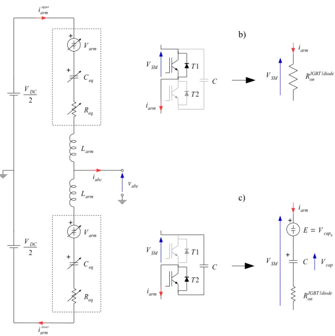
Figure 4.4 a) MMC arm circuit, b) off-state SM, c) on-state SM . . . 52

Figure 4.5 An IP block representing one phase of the MMC . . . 55

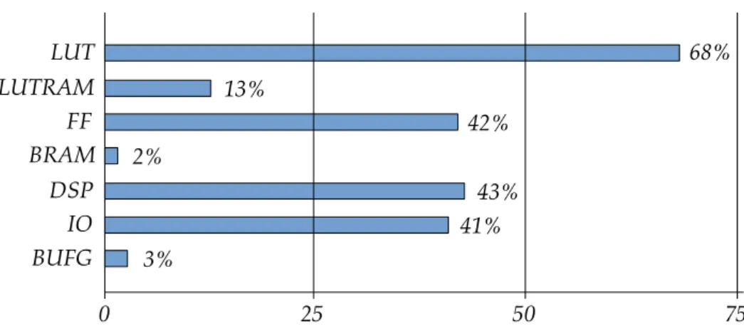
Figure 4.6 FPGA resources usage when using no directives or pragmas . . . 58

Figure 4.7 Execution time comparison . . . 59

Figure 5.1 Complete IP block diagram showing signal and data paths . . . 64

Figure 5.2 FPGA hardware resources utilisation (%) . . . 66

Figure 5.3 Vivado Block Design . . . 68

Figure 5.4 Zynq Processing System IP . . . 69

Figure 5.5 MMC HIL model IP . . . 69

Figure 5.6 Capacitor voltage eRTS IP . . . 71

Figure 5.7 PWM Generator IP . . . 72

Figure 5.8 CIC filter IP . . . 72

Figure 5.9 CIC filter structure for decimation (N=3, M =1) . . . 73

Figure 5.10 CIC converter to float IP . . . 74

Figure 5.11 Capacitor overvoltage alarm IP . . . 75

Figure 5.12 XADC IP . . . 76

Figure 5.13 State Machine diagram including software initialization, MMC capaci-tor charging, MMC normal operation and data retrieval . . . 77

Figure 5.14 Evolution of the input, output and capacitor voltages through the exe-cution states . . . 79

Figure 5.15 PSCAD detailed model of the MMC . . . 83

Figure 5.16 MMC model validation: Output currents . . . 85

Figure 5.17 MMC model validation: Phase output voltages . . . 86

Figure 5.18 MMC model validation: Upper capacitor voltages . . . 87

Figure 5.19 MMC model validation: Lower capacitor voltages . . . 88

Figure 5.20 MMC model validation: Phase output currents - Detail . . . 89

Figure 5.21 MMC model validation: Phase output voltages - Detail . . . 90

Figure 5.22 MMC model validation: Upper capacitor voltages - Detail . . . 91

Figure 5.23 MMC model validation: Lower capacitor voltages - Detail . . . 92

Figure 5.24 Energy controllers . . . 92

Figure 5.25 Current controllers . . . 93

Figure 5.26 Capacitor balancing controllers . . . 93

Figure 5.27 MMC IP working as HIL . . . 94

Figure 5.28 Input voltage and HIL estimated output voltage and currents - Com-plete simulation . . . 94

Figure 5.29 HIL estimated capacitor voltages - Complete simulation . . . 95

Figure 5.30 HIL estimated capacitor voltages - Capacitor oscillations . . . 95

Figure 5.31 Input voltage and HIL output voltage and currents. At 4.5s the control starts operating . . . 96

Figure 5.32 Input voltage and HIL estimated output voltage and currents. Load switched in at 6.5s . . . 96

Figure 5.33 Input voltage and HIL estimated output voltage and currents. Load switched out at 7.5s . . . 97

Figure 5.34 Test bench input and output voltages and output currents (from 0s to 5.5s) . . . 98

Figure 5.35 Test bench capacitor voltages (from 0s to 5.5s) . . . 98

Figure 5.36 Test bench input and output voltages and output currents(from 3.48s to 3.6s) . . . 99

Figure 5.37 Test bench capacitor voltages (from 3.48s to 3.6s) . . . 99

Figure 5.38 eRTS for fault-tolerant control diagram . . . .101

Figure 5.39 Current offset observer and Capacitor voltage eRTS diagram . . . .102

Figure 5.40 eRTS upper cell voltage estimation during normal operation . . . .103

Figure 5.41 eRTS lower cell voltage estimation during normal operation . . . .103

Figure 5.42 eRTS upper cell voltage estimation during change from normal opera-tion mode to fault mode at 5.5s . . . .104

Figure 5.43 eRTS lower cell voltage estimation during change from normal opera-tion mode to fault mode at 5.5s . . . .105

Figure 5.44 Upper capacitor voltage error . . . .105

Figure 5.45 Lower capacitor voltage error . . . .106

Figure 5.46 eRTS upper cell voltage estimation during change from normal opera-tion mode to fault mode at 5.5s - Detail . . . .106

Figure 5.47 eRTS lower cell voltage estimation during change from normal opera-tion mode to fault mode at 5.5s - Detail . . . .107

Figure 5.48 Voutreconstruction . . . 108

Figure 5.49 Voutreconstruction switching the Capacitor voltage eRTS in at 5.5s . . . 108

Figure A.1 Test bench main diagram - Control system . . . .120

Figure A.2 Test bench main diagram - Power converter . . . .120

Figure A.4 Rack picture - Front . . . .122

Figure A.5 Rack picture - Back . . . .122

Figure A.6 Half-Bridge sub-module picture . . . .123

Figure A.7 Half-Bridge rack diagram . . . .123

Figure A.8 Control board picture . . . .124

Figure A.9 Fiber optics interface . . . .125

Figure A.10 Protection board . . . .126

Figure A.11 Protection board diagram . . . .126

Figure A.12 Current and voltage sensor . . . .127

L I S T O F TA B L E S

Table 2.1 FPU instruction throughput and latency cycles . . . 18

Table 3.1 Number of operations to be executed . . . 37

Table 3.2 Best execution times (per iteration) on the ARM . . . 39

Table 3.3 Latency and area utilisation on the Zynq-7020 . . . . 40

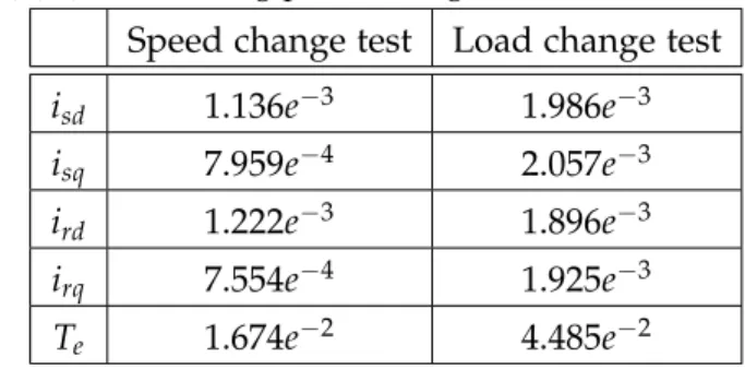
Table 3.4 64-bit floating-point average errors (software version) . . . 40

Table 3.5 32-bit floating-point average errors (software version) . . . 41

Table 3.6 32-bit floating-point absolute average errors (hardware version) . . . 42

Table 3.7 32-bit fixed-point absolute average errors (hardware version) . . . 43

Table 3.8 FPGA hardware resources utilisation (32-bit) . . . 43

Table 4.1 Execution time (in µs) . . . 57

Table 4.2 Precision results for va . . . 59

Table 5.1 FPGA hardware resources utilisation . . . 66

Table 5.2 HLS IPs execution times using a 100MHz clock . . . 66

Table 5.3 MMC HIL Execution time per state . . . 81

L I S T E D E S S Y M B O L E S

ADC Analog-to-Digital Converter

AMBA Advanced Microcontroller Bus Architecture

AXI Advanced Extensible Interface

CPLD Complex Programmable Logic Device

DAC Digital-to-Analog Converter

DDR Double Data Rate memory

DFIG Doubly-Fed Induction Generator

DMA Direct Memory Access

ERTS Embedded Real-Time Simulator

FPGA Field-Programmable Gate-Array

HB Half-Bridge

HDL Hardware Description Languages

HLS High-level Synthesis

I/O Input/Output

IP Intellectual Property

MMC Modular Multi-level Converter

MSPS Mega Sample Per Second

OCM On-chip Memory

OPAMP Operational Amplifier

PCB Printed Circuit Board

PL Programmable Logic

PS Processor System

PWM Pulse-Width Modulation

QoS Quality-of-Service

RT Real-Time

RTL Register Transfer Level

SM Submodule

SoC System-on-Chip

VHDL VHSIC Hardware Description Language

XADC Xilinx Analog-to-Digital Converter

Part I

1

G E N E R A L I N T R O D U C T I O N

In the course of the last two decades, real-time digital simulation has been under the focus of important research in almost any area of engineering. Its aim is mainly to provide control en-gineers with another testing scenario right after the offline simulation verification –but much closer to reality than this one, before its trial and deployment on the real plant. Actually, a real-time simulation differs from a standard offline simulation in that the system behavior is simulated in natural time by implementing its dynamical model on hardware. As a con-sequence, the design of a Real-Time Simulator (RTS) includes additionnal constraints to the development cycle which can be classified in three levels: (i) the modeling of the system to be controlled, (ii) its digital realization, and (iii) its digital implementation.

These RTS have been used mainly as Hardware-in-the-Loop (HIL) testing of controllers, where the plant model is executed at the same pace as the real system providing a similar dynamic response. Even though the focus of this thesis is very much related with them, its aim goes a bit further, where these RTS will be embedded within the controller to provide additional functionalities. These Embedded Real-Time Simulators (eRTS) could play several roles like obser-vators, estimators, diagnosis and health-monitoring, or fault-tolerant and sensorless control to mention some of them.

Nevertheless, when implementing such model-based eRTS, the main concern is how to balance between the accuracy of the model, the system dynamics, the simulation time-step (implicitly the execution time) and the needed mathematical computations to be executed in the chosen digital platform. The main challenge when designing these simulator Intellectual Properties1

(IPs) is to cope with their complexity having in mind that, in the case of embedded systems, the available hardware resources are limited. Moreover, this challenge is increased by the requirement of very short simulation time-steps when simulating power electronics [2].

To bring technological solutions to these implementation issues, for some years there has existed a new kinds of devices called System-on-Chip (SoC) which integrate in the same device CPU-based processor cores along with a Field-Programmable Gate Array (FPGA) fabric and other peripherals such as ADCs, DACs, DMAs, and hardware interfaces which provide these platforms with great connectivity capabilities.

Alongside these devices, the design tools have evolved as well aiming to reduce develop-ment time of the increasing complexity of nowadays controllers, providing professional tools that ease the utilisation and exploitation of SoC devices.

1 An IP core is a block of logic or data that is used in making an FPGA or Application-Specific Integrated Circuit

(ASIC) for a product. As essential elements of design re-use, IP cores are part of the growing Electronic Design Automation (EDA) industry trend towards repeated use of previously designed components. Ideally, an IP core should be entirely portable –that is, able to easily be inserted into any vendor technology or design methodology. Universal Asynchronous Receiver/Transmitter (UART), Central Processing Units (CPU), Ethernet controllers, Universal Serial Bus (USB) and PCI interfaces are all examples of IP cores [1].

1.1 t h e s i s o b j e c t i v e s a n d au t h o r c o n t r i b u t i o n s

The goal of this dissertation is then to evaluate and analyze the capabilities of these kinds of devices and the software tools that come with them for the implementation of accurate and reliable eRTS of electrical systems. In this work, the Zynq-7000 All Programmable SoC from Xilinx Inc. has been selected and its choice will be motivated later on.

To this purpose, two case applications have been chosen. Offshore Wind farm are composed of several subsystems. Among them, electrical machines (wind generators) and power elec-tronic systems (power converters) are significantly different in terms of requirements, and quite representative of what SoC devices can be used for.

Regarding the electrical machine, the decision of choosing a Doubly-fed Induction Generator (DFIG) has been taken because it is a quite popular generator used as wind turbines and it has a representative model complexity compared to other electromechanical systems [3]. The

specific application is a DFIG working as an islanded generator and feeding a three-phase RL load [4,5,6,7].

Concerning power electronics systems, some might think that it would have been more appropriate to use the classical two-level power converter that is usually connected to the DFIG in order to test the device in a complete power electronics application. However, this work has already been done; it can be found extensively in the literature, and it does not have the amount of complexity to evaluate the full capabilities of a SoC device [8,9,10]. Therefore,

in this work it has been decided to use a Modular Multilevel Converter (MMC) [11]. The aim of

choosing it is however to use a scalable power converter, with a much more complex structure in order to exploit the device capabilities at maximum, coping with the eRTS requirements of speed, computational power, and degree of parallelism [12,2,13,14].

In more detail, the idea is to have one –or several– IP blocks which estimate: e.g. stator and rotor currents and voltages, phase output voltages, arm and load currents, Half-Bridge (HB) capacitor voltages, etc.; based on other measured magnitudes. One of the most interesting applications these IP blocks could be utilized for is in the context of fault-tolerant embedded controllers, where these estimated variables would be used in case of a sensor fault. Further-more, they could also be adopted as estimators, observers, or also applied for diagnosis and health-monitoring [8, 15], without forgetting HIL applications for testing the control before

its deployment on the real plant [16,17,18,19,8], and sensorless control [20,21,22,23].

Accordingly, several IP blocks will be developed. On one hand, by the creation of several DFIG models using two different discretization methods and exploring whether is more suit-able to execute the coded algorithms either in software using the Processing System (PS), in hardware using its Programmable Logic2

(PL), or a collaboration between both. And on the other hand, by the conception of various MMC models to estimate different converter vari-ables, modifying the number of cells per arm to exploit all the computational power of the device.

Moreover, a deep exploration of the Vivado HLS software tool will be performed as well aiming to reduce the execution time at maximum, using different data formats (fixed- and floating-point) and data widths (64- and 32-bit) for the internal and external variables. The device performance will be compared in terms of execution time, resources utilisation and precision of the calculations.

2 A Programmable Logic Device (PLD) is an electronic component used to build reconfigurable digital circuits. Unlike a logic gate, which has a fixed function, a PLD has an undefined function at the time of manufacture. Before the PLD can be used in a circuit it must be programmed, that is, reconfigured [24].

1.2 thesis outline 5

In this study, a total of three boards mounting two different Zynq versions will be uti-lized. The ZedBoard3

and the MicroZed4

development boards manufactured by Avnet Inc., both mounting a Zynq-7020 classified as mid-range with an Artix-7 equivalent FPGA fabric, will be used for the DFIG study and for the experimental tests respectively. For the MMC case evaluation however, the ZC706 Evaluation Kit produced by Xilinx Inc. will be utilized. The lat-ter mounts a high-end Zynq-7045 having a Kintex-7 equivalent FPGA fabric with considerably more hardware resources.

To conclude, an MMC test rig has been developed and used to prove a real-world imple-mentation of eRTS. First, by using one IP to perform HIL validation of the controller before its deployment on the real plant; and second, by implementing a capacitor voltage estimator for fault-tolerant control.

This thesis work is mainly focused on the digital implementation issues of eRTSs. In fact, the proposed work can be seen as an extension of Dr. Dagbagi’s thesis [25] where the focus

was limited to full-hardware FPGA-based implementation of eRTSs. However, the implemen-tation constraints have been extended to consider SoC devices, which allow full-hardware, full-software and mixed hardware/software solutions.

1.2 t h e s i s o u t l i n e

The rest of this thesis dissertation is organized as follows: Chapter2presents the State of the

Art and introduces the main problems linked to the development of eRTSs. Then it focuses on the digital implementation by presenting the SoC technology and the programming tools linked to them. Chapter 3 is dedicated to eRTSs for electromechanical systems, hence the

DFIG case. Chapter 4 is devoted to the eRTS for power electronic systems, therefore the

MMC case. In Chapter5an exhaustive experimental validation of the MMC implementation

is performed. Finally, Chapters 6 and 7 are left for general conclusions and future work

respectively. At the end of this document Appendix A can be found with the description of the test bench, and Appendix Bwith the parameters of the state space model utilised in the experimental tests.

3 Official website zedboard.org. 4 Official website microzed.org

2

S TAT E O F T H E A R T

2.1 i n t r o d u c t i o n

This chapter discusses the main problems linked to the development of eRTS of electrical systems. They can be located at the main development stages of the eRTSs and can be classi-fied as follows: (i) Selection of the system’s mathematical model, (ii) digital realization of this model and (iii) its digital implementation.

1. Modeling. A model of the plant has to be found, with a good approach to emulate the system’s behavior using appropriate equations. Regarding power systems dynamics, they can be divided into two groups:

• Electromechanical and electromagnetic systems, which have relatively slow dy-namic response

• And power electronics systems, which have much more fast dynamics

2. Digital realization. In this step have to be chosen: a –constant– time-step, a numerical solver (explicit or implicit), and an appropriate data format (fixed- or floating-point), aiming always at the highest level of precision considering the computational power available.

3. Implementation. The last step is where the simulation platform to be used has to be decided. There exist many different possibilities ranging from powerful multi-core pro-cessors, FPGAs, or SoC devices to mention the most commonly used nowadays. The methodology when programming each of these platforms differ significantly and so do the software tools utilised. Moreover, the programming languages are also a big issue specially when FPGAs are involved.

2.2 w h at i s a n e m b e d d e d r e a l-time simulator?

The real-time concept has been extensively used by the industry but worn and utilised inap-propriately most of the time by the general public. According to [26] “A real-time system can

be described as one which controls an environment by receiving data, processing them, and returning the results sufficiently quickly to affect the environment at that time”. By using this description one could think that every controller is implemented in real-time. In regard to the subject we are on, this other more appropriate and specific definition is preferred: “Real-time is an adjective describing a system in which results and feedback follow input with no noticeable delay from the sys-tem’s point of view”. Accordingly, the timing requirements will rely upon the dynamics of the system under study.

A system is said to be in real-time if the total correctness of an operation depends not only on its logical fidelity, but also on the time in which it is performed. According to [27],

Deadline Time

Soft RT system Firm RT system Hard RT system Usefulness

Figure 2.1: Real-Time systems classification

real-time systems, as well as their deadlines, are classified by the consequence of missing a deadline:

• Hard: any missed deadline is a total system failure

• Firm: infrequent deadline misses are tolerable, but may degrade the system’s Quality of Service1

(QoS)

• Soft: The usefulness of a result degrades after its deadline, thereby degrading the sys-tem’s QoS

Figure2.1shows a representation of this classification.

Moving forward on the definition, a Real-Time Simulator (RTS) can be seen as a digital entity that mimics a real-world system or a part of it, which is executed at a rate that matches the one of the real process. As it will be explained later, this digital entity is executed at a constant time-step. Any missed deadline due to implementation issues is not tolerated, causing a simulation failure. Hence, RTSs can be classified as hard real-time systems.

When applied to electrical systems, RTS are mostly implemented in the context of Hardware-in-the-Loop (HIL) testing of the system controller in order to validate it in every operating condition, which would not be possible using only experimental setups [18,19,16,17].

How-ever, an RTS can also be embedded within the controller of the system in what is known as an Intellectual Property2

(IP) to play several roles like observators, estimators, model-based diagnostics, fault-tolerant and sensorless control, health monitoring, etc. It is in this context where such IP modules are called Embedded Real-Time Simulators (eRTS) [25,8,6,28,7,14].

Apart from the execution rate, another constraint when designing an eRTS is to cope with its complexity having in mind that, in the case of embedded systems, the available hardware resources of the digital platform are limited.

Moreover, this challenge is increased by the requirement of very short simulation time-steps when simulating power electronics [15]. This is the reason why at each development stage,

1 Description or measurement of the overall performance of a service.

2 An IP core is a block of logic or data that is used in making an FPGA or Application-Specific Integrated Circuit

(ASIC) for a product. As essential elements of design re-use, IP cores are part of the growing Electronic Design Automation (EDA) industry trend towards repeated use of previously designed components. Ideally, an IP core should be entirely portable - that is, able to easily be inserted into any vendor technology or design methodology. Universal Asynchronous Receiver/Transmitter (UART), Central Processing Units (CPU), Ethernet controllers, Universal Serial Bus (USB) and PCI interfaces are all examples of IP cores [1].

2.3 erts development (i) : system modeling 9

designer must rigorously consider a set of constraints linked to: (i) the chosen model of the system part to be RT simulated; (ii) its digital realization and (iii) its implementation on the targeted digital platform.

In the following, these development constraints will be discussed. Since the outline of this thesis is more about the implementation issues, an important focus will be given to the de-scription of the available SoC FPGA platforms and their value-added to this context.

2.3 e r t s d e v e l o p m e n t (i) : system modeling

To face today’s society and industry demands, the electrical systems have been the focus of intensive research starting from power generation, storage, until its consumption. As a con-sequence, a wide range of increasingly complex machine drives, power electronic converters and their controllers are now available in the market. This trend makes their design very chal-lenging since the time-to-market and the growing development cost must also be considered. All these reasons make the real-time digital simulation of these electrical systems mandatory in modern design cycles.

The first thing that influences the quality of a real-time simulation is the chosen model. It has to be properly formulated in order to represent the static and dynamic behavior of the system accurately. However, it has to be understood that a mathematical model of a system is a simplified representation of the reality. This simplification has to be done mainly because of two reasons: (i) models can become extremely complicated and hence, their development time can be significantly long; and (ii), these models have to be executed in a digital device, so execution time and resources must be considered. Therefore, neglecting physical phenomena that occur in the system (e.g. saturations, core losses, saliencies, power converter switching, skin effects, etc.) has to be assumed in most of the cases. This becomes even more impor-tant when considering RTS where the execution time of the mathematical model is a critical constraint.

An electrical system can be described as a set of interconnected elements that have different characteristics and dynamics. Naming them and starting from slow to fast dynamics: thermal dynamics, electromechanical dynamics, electrical dynamics, electromagnetic dynamics, and power electronics dynamics. Due to their wide gap between them, these phenomena can be grouped in two: fast dynamic systems considering only the power electronics systems, and slow dynamic systems grouping the rest [25]. In this dissertation, an example representing each of

the groups will be studied.

2.4 e r t s d e v e l o p m e n t (ii) : digital realization

Besides its mathematical modeling, the real-time simulation of an electrical system is also conditioned by the digital realization of the chosen models. This consists in selecting the appropriate numerical solver, the right simulation time-step, and the numerical representa-tion of the processed data. The choice has to consider: the complexity (number of operarepresenta-tions to implement), accuracy (contrasted to the original continuous-time model); numerical stabil-ity (the system may become unstable due to proximstabil-ity to singularities of various kinds or by growth of round-off errors or small fluctuations in initial data); and respect of real-time operation (computation time shorter than the chosen time-step).

4

4

Exec.

ERTS Exec.ERTS

Exec.

ERTS ERTSExec. Executecontrol

CIC int. (5us)

values available _Read

XADC Write to ERTS inputs

Read & Save ERTS outputs

Read

XADC Write to ERTS inputs

Read & Save

ERTS outputs Send control signals to PWM

Apply outputs and read inputs

Solve model equations

2

3

...

_...

5us 5us 5us 5us

100us 5us 5us 5us 100us 5us

...

95us 100us 105us 110us 200us

1

1

2

3

4

2

3

1

...

Total time-step Time

Figure 2.2: Real-time execution tasks

2.4.1 Numerical solver

The numerical solvers use a set of integration algorithms that approximate, based on Taylor series, the continuous-time differential equations of the plant. The approximation order has a huge impact, but if only the first-order approximation methods are considered, two cate-gories can be differentiated: explicit and implicit methods. The explicit methods calculate the state variables3

of the current time-step based only on previous values. Conversely, implicit methods compute the state variables based on current and previous values. More details and quantitative comparisons have been discussed in [25].

2.4.2 Time-step selection

The right choice of the real-time simulation time-step is crucial, specially when explicit meth-ods are in use. They might become unstable if the simulation time-step is too short. Implicit methods do not present this problem as far as all the continuous-time real poles are negative [29].

As previously introduced, it is assumed a discrete-time and constant time step. This means that during a discrete-time simulation, time moves forward in steps of equal duration. This is known as fixed time-step simulation [30]. However, other solving techniques exist which

use variable time-steps. Such techniques are used for solving high frequency dynamics and non-linear systems, but they are not suitable in the context of RTSs because of important implementation issues [31]. In addition, the required time to compute the model at a given

time-step must be shorter than the wall-clock duration of the chosen time-step. Therefore, if the simulator operations are not all achieved within the required time-step, the RTS commits an overrun and the simulation is considered as non-valid [26].

As shown in Figure 2.2, for each time-step, the simulator must execute the same series of

tasks: 1) apply previous iteration outputs and read current iteration inputs, 2) solve model equations, 3) generate outputs and 4) wait for the start of the next iteration. So in order to guarantee a real-time execution, the amount of time needed to perform these operations should be less than the total time-step.

The four most important selection criteria when defining the time-step duration are the following:

3 A state variable is one of the set of variables that are used to describe the mathematical “state” of a dynamical

2.4 erts development (ii) : digital realization 11 0 0.2 0.4 0.6 0.8 1 1.2 1.4 1.6 1.8 2 0 0.2 0.4 0.6 0.8 1 1.2 1.4 Continuous Discrete (T_s= 0.05 τ) Discrete (T_s= 0.1τ) Discrete (T_s= 0.5τ) Time (seconds) Amplitude

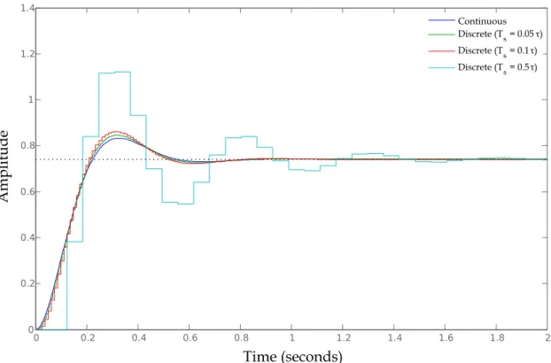
Figure 2.3: Effect of time-step selection when discretizing

• System dynamics. According to [26,32], when an electromagnetic element is of concern,

a time-step between 5% to 10% of the smallest time constant has to be chosen. To give an idea, most mechanical systems –which have slow dynamics– require time-steps from 1ms to 10ms, whereas electromagnetic transient simulation with frequency content up to 10kHz, typically require a simulation time-step around 10µs. Furthermore, if the objective is to accurately simulate fast-switching power electronic devices, the timing requirements can be in the order of 250ns without interpolation, or 10µs if an interpola-tion technique is utilized [32,33]. In Figure2.3is shown how different time-steps affect

the discrete-time system’s similarity with the continuous-time version.

• Interfacing errors. When considering switching elements which are interfaced with a controller, the power converter RTS can respond to its control signals only at each simu-lation time-step [34]. As a result, switching events that occur between two steps cannot

be detected and therefore errors are inevitably introduced to the simulation results. To avoid this problem, the time-step should be at least 100 times shorter than the switching period [35]. Figure 2.4 shows how the PWM sampled signal fidelity decreases as the

sampling period increases. Note that Ts3 =2Ts2 =4Ts1.

• Numerical stability. Whatever the numerical solver is, even if it is unconditionally stable4 , when the time-step decreases, the poles of the discrete-time model move closer to the stability limit (i.e.,|z| =1). Hence, poles become very sensitive to variations caused by limited precision data quantification [36]. These variations may then lead to instability

4 According to [29], A-stable discretization methods are unconditionally stable if all continuous-time poles are stable, i.e. they are placed in the negative part of the s-plane. All implicit methods have this characteristic.

Deadline Time Soft RT system Firm RT system Hard RT system Usefulness Sampling Ts1 Time Ts2 Ts3 PWMcont. PWM1 PWM2 PWM₃

Figure 2.4: Interfacing errors

especially when fixed-point format is used. Hence, care should be taken when choosing the amount of fractional bits and its representation. Moreover, the growth of round-off errors or small fluctuations in initial data could also affect the stability of the system [37].

• Real-time operation. Logically, when considering a real-time simulation, the time-step must be short enough to reproduce system’s behavior, but at the same time, sufficiently long to allow processing of the model equations (see Figure2.2). Accordingly, to

guaran-tee real-time operation, the processing time must be shorter than the chosen time-step [26].

2.4.3 Data representation

Regarding the numerical data representation, fixed- or floating-point can be adopted. The first uses between 3 to 4 times less hardware and is 3 to 4 times faster [38]. However, the price

to pay is accuracy. With floating-point representation the range of the data is much more broader but the price to pay is complexity of floating-point operations and thus, both area utilisation and computation time increases.

2.5 e r t s d e v e l o p m e n t (iii) : digital implementation

Once the importance of selecting the right model, the appropriate numerical solver, a suitable time-step, and the right data format has been explained, the final step that influences the performance of a real-time simulation is its digital implementation. The main challenge from the application’s point of view is to find an appropriate platform able to handle the complex-ity of the simulated system and ensure the required timing performances, i.e. providing a simulation time-step small enough to properly simulate the highest system dynamics.

Along this line, many performance digital platforms are available in the market. They inte-grate powerful multi-core processors where the number of CPUs and other components can be arranged on demand by the manufacturer regarding system’s scale, complexity, number of I/Os, timing requirements, cost, etc. The most widely known companies providing

commer-2.5 erts development (iii) : digital implementation 13

cial real-time simulators are RTDS Technologies5

and Opal-RT6

. The first are more focused on power systems applications whereas the second excel on power electronic based applications.

From the designer’s point of view, these platforms are provided with a set of software tools that allow creating the system’s model, setting up the simulation, controlling and modifying the system parameters during simulation, acquire data, and analyze its results. Two examples can be RTDS Simulator from RTDS Technologies, and HYPERSIM from Opal-RT. Besides these tools, which are specific to each manufacturer, they often provide as well toolboxes that allow using their hardware in traditional simulation tools like MATLAB/Simulink from Mathworks7

. As far as digital implementation is concerned, using FPGAs for real-time simulation has been a big trend in the last few years [18,19,35,39,40]. This approach has many advantages.

First, computation time is almost independent of the size of the system because of the parallel nature of FPGAs. Second, overruns cannot occur when the model is implemented in hardware once timing constraints are met during the design process. And finally, the simulation time-step achieved can be in the order of few hundred of nanoseconds. However, there are still limitations on model size since the number of gates and their interconnections are limited.

Hence, to boost timing performances these commercial platforms are also equiped with FPGA-based boards, which have been successfully integrated because of the following rea-sons:

• Parallel computational capability. Works [35,39,40,9] show how these kinds of devices are

used in the real-time simulation of electrical systems with ultra-fast transients such as high-frequency IGBT-based power converters. Taking advantage of the inherent paral-lelism of FPGAs, the computation time is reduced setting small time-steps in the order of 1µs or less.

• Additional hardware resources. These devices include distributed memories, Digital Sig-nal Processor (DSP) blocks, high speed I/Os, ASig-nalog-to-Digital Converters (ADC), Digital-to-Analog Converters (DAC), logic blocks, etc., which give the possibility to implement complex models like power converters with large number of switches [41], or using the

combination of multiple FPGA boards to simulate large-scale systems [42].

• New design tools. The traditional way of programming these kinds of devices was using Hardware Description Languages (HDL). The most widely utilised are VHDL, Verilog and SystemC. However, the use of these languages can be seen as a disadvantage since con-trol and software engineers might not be particularly familiar with them. To overcome this issue, two kinds of software tools are available in the market. Most commercial simulation platforms allow today to program the FPGAs by using graphical tools such as Xilinx System Generator from Xilinx, DSP Builder toolbox from Intel8

, or the LabVIEW FPGA Module from National Instruments. The second group are High-Level Synthesis (HLS) tools let the designers to work at a higher abstraction level by specifying the behavior of an algorithm using C, C++ or SystemC. Additional information regarding this last set of tools can be found in Section2.7.

As introduced earlier, these high-performance platforms are most of the time dedicated to HIL testing during the design of digital controllers [18,19,16,17]. However, their cost is not

always taken into account. Additionally to the reduction of the development time and the

5 Official website rtds.com 6 Official website opal-rt.com 7 Official website mathworks.com

8 Intel recently bought Altera Corporation, an American manufacturer of programmable logic devices who released

verification of the controller in every situation, the other primary objective of a HIL test is to achieve a high level of correspondence with the real plant. This implies utilizing detailed and complex algorithms running at very short time-steps. The consequence is the use of powerful but costly digital platforms [41, 43]. Nevertheless, The use of such expensive devices is not

acceptable in the case of embedded applications where eRTSs are not only developed for HIL testing but also embedded within digital controllers [8,25,7,14].

Consequently, the constraints linked to the real-time simulation discussed in the former Section are strengthened by those of embedded systems such as cost, power consumption, reliability, size, and flexibility. To bring solutions to this new field, SoC devices including FPGA fabric are surely one of the most promising technologies. The following Section tries to prove it by describing these devices and giving an overview of the design opportunities that they offer thanks to their versatile architecture and improved design tools.

2.6 s y s t e m-on-chip devices

A wide and diversified range of powerful platforms are available nowadays in the market. Among them, recent SoC devices are surely the most promising since they bring a new design paradigm thanks to their heterogeneity and computational power. Heterogeneity because they include in the same chip general-purpose processors and an FPGA fabric associated to several peripherals like ADCs or DACs; and computational power thanks to these potent hard-processors plus the many capabilities the PL offers, which can increase massively the computing speed of the whole system.

Considering all these properties, one can easily see that SoC-based eRTS offer much more flexibility compared to the pure hardware FPGA-based eRTS approach studied in [25]. To

provide clear examples about it, with this new technology it is possible to go with a full-software implementation (everything runs in the processor or processors), a full-hardware one (all is computed in the FPGA fabric), or a hardware-software co-design where only the heavy calculations are performed in hardware (also known as a hardware accelerator).

2.6.1 General overview

To cite some of these new SoC devices, the first version of Microsemi’s SmartFusion SoCs features an ARM Cortex-M3 processor clocked at 100MHz, an FPGA fabric, and other pro-grammable analog circuitry [44]. The processor is the actual industry-leading 32-bit processor

for highly deterministic real-time applications [45]. Its FPGA part is based on their ProASIC3

architecture, ranging between 60.000 to 500.000 system gates with up to 350MHz system performance, embedded SRAMs and FIFOs and up to 128 FPGA I/Os supporting LVDS, PCI, PCI-X and LVTTL/LVCMOS standards [46]. The programmable analog has high-performance

analog signal condition blocks with voltage, current and temperature monitors, 12-bit ADC and DAC converters, up to ten 15ns high-speed comparators, and up to 32 analog inputs and 3 analog outputs. They offer as well the SmartFusion2 (diagram shown in Figure2.5) with

lower power consumption, higher security, and better reliability for safety critical and mission critical systems [47].

Intel –formerly Altera– offers a full-range SoC FPGA product portfolio spanning high-end, mid-range, and low-end applications [48]. Their high-end Stratix 10 SoC mount the powerful

64-bit quad-core ARM Cortex-A53 processor [49], whereas the Arria 10, Arria V and Cyclone V

SoCs feature a 32-bit dual-core ARM Cortex-A9 processor [50], a significantly more powerful

2.6 system-on-chip devices 15

Figure 2.5: Microsemi’s SmartFusion2 SoC FPGA [credit: Microsemi Corp.]

with two embedded hardware accelerators per core, which will be described afterwards: the NEON Single Instruction, Multiple Data (SIMD), capable of executing the same mathematical operation on several registers in parallel [51]; and the VFPv3 (in Cortex-A9) and VFPv4 (in

Cortex-A53), two Floating-point Units (FPU), which can compute operations with very few clock cycles in either 32- and 64-bit precision [52,53]. These two units, initially developed and

broadly used in media processing, can be configured and used to execute intensive operations –like matrix multiplications and matrix inversions– reducing the execution time significantly compared to sequential operations in common processors or DSPs. Moreover, they are com-posed as well of configurable L1 caches up to 64kB of memory with a system coherency support using the Accelerator Coherency Port (ACP), and hardened floating-point DSP blocks capable of processing rates up to 1.5 TFLOPS9

and power efficiency up to 40 GFLOPS/Watt. However, Intel’s SoC does not come with a built-in ADC. The Cyclone V SoC diagram is shown in Figure2.6.

The last example of SoC devices available in the market, which is included in this thesis work, is the Zynq All Programmable SoC produced by Xilinx, which main diagram is shown in Figure2.7. They offer a broad portfolio ranging from single-core 32-bit ARM Cortex-A9 plus an

Artix FPGA fabric, passing through a double-core version with the FPGA hardware available in both technologies Artix and Kintex. Recently, they released the Zynq UltraScale+ featuring dual- and quad-core ARM Cortex-A53 (64-bit architecture), another version including as well a dual-core ARM Cortex-R5 deterministic real-time microcontroller, plus the highest-end ver-sion which also comes with a GPU10

Mali-400 MP2 supporting the H.264-H.265 video codec. Wistfully, Xilinx has not included in any of the Zynq UltraScale+ versions the double 12-bit ADC, 1MSPS11

ADCs present in the older Zynq-7000 devices [54].

9 In computing, floating-point operations per second (FLOPS) is a measure of computer performance, useful in fields

of scientific computations that require floating-point calculations.

10 A Graphics Processing Unit (GPU) is a specialized electronic circuit designed to rapidly manipulate and alter

memory to accelerate the creation of images in a frame buffer intended for output to a display device. 11 Millions of Samples Per Second (MSPS).

Figure 2.6: Intel’s Cyclone V SoC [credit: Intel Corp.]

2.6 system-on-chip devices 17

Figure 2.8: NEON operations [credit: Xilinx Inc.]

2.6.2 ARM Cortex-A9 hardware accelerators

When implementing an RTS, the processing accuracy and execution time are the most critical parameters [8,55,22]. Indeed, the choice between using floating- or fixed-point data format is

directly related not only with the accuracy of the calculations, but also with the time needed to execute them. As previously introduced, the ARM Cortex-A9 present in the Intel and Xil-inx’s products, have two powerful FPUs [52], one per core, which are capable of computing

operations with very few clock cycles either in 32- or 64-bit precision –see Table2.1.

Addition-ally, these powerful processors come as well with two NEON SIMD units which can execute the same mathematical operation on several registers in parallel [51], decreasing significantly

the algorithm execution time as it will be demonstrated later on. These two units can be con-figured and used to execute intensive operations reducing the execution time significantly.

2.6.2.1 The NEON SIMD

NEON technology is a 128-bit SIMD architecture extension of the ARM Cortex-A9 series pro-cessors, designed initially to provide flexible and powerful acceleration for consumer multi-media applications [51]. It has 32 registers, 64-bits wide (dual view as 16 registers, 128-bits

wide), which are shared with the FPU.

It can perform packed SIMD processing –see Figure2.8:

• Registers are considered as vectors of elements of the same type

• Data types can be: signed/unsigned 8-bit, 16-bit, 32-bit, 64-bit, and single precision floating-point

• Instructions perform the same operation in all lanes

2.6.2.2 The VFPv3 FPU

This FPU provides hardware support for floating-point operations in half-, single- and double-precision floating-point arithmetic [52]. The FPU fully supports the basic instructions shown

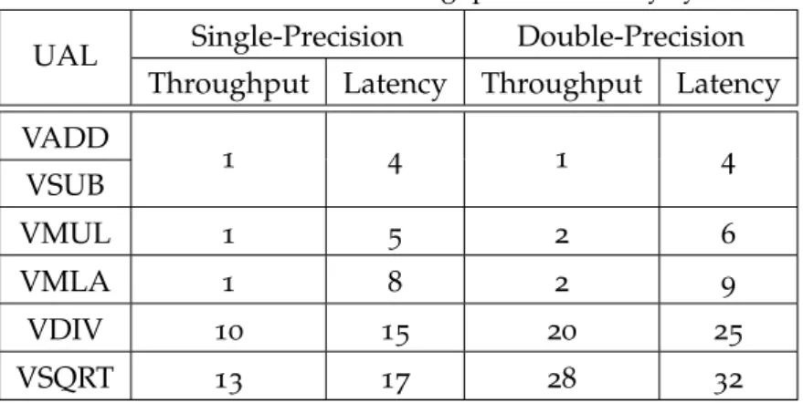
in Table 2.1 along with their corresponding latency12 and throughput13 for either 32- and

64-bit floating-point formats.

12 Number of clock cycles to process an operation.

Table 2.1: FPU instruction throughput and latency cycles

UAL Single-Precision Double-Precision

Throughput Latency Throughput Latency VADD 1 4 1 4 VSUB VMUL 1 5 2 6 VMLA 1 8 2 9 VDIV 10 15 20 25 VSQRT 13 17 28 32 2.6.3 PS-PL interfacing

Regarding the interface between PS, PL, and the additional peripherals of the devices pre-sented above, all of them use ARM’s Advanced Microcontroller Bus Architecture (AMBA) open-standard, on-chip interconnect specification. However, each manufacturer uses a different version. Microsemi uses the AMBA 2, a 1999 protocol called Advanced High-performance Bus (AHB), a single clock-edge protocol. Intel chose the AMBA 3 specification from 2003, which included the Advanced eXtensible Interface (AXI3), a high-performance, high-clock frequency system designs that uses separate address/control and data phases, supports unaligned data transfers and burst based transactions with only start address issued. Xilinx opted for the AMBA 4 specification released in 2011, which included the AXI4 defining three new different protocols: AXI4-Master, AXI4-Lite, and AXI4-Stream. The AXI4-Master is an improved version of the AXI3 protocol, allowing bigger burst transactions and QoS signals among other en-hancements. The AXI4-Lite is a simpler version of the AXI4-Master that uses less hardware resources and is intended to be used mainly for control and configuration purposes. Both are memory mapped protocols, where the read/write transactions contain the destination ad-dresses. Finally, the AXI4-Stream is the simplest and fastest interconnection, where there are no addresses involved, uses one single channel and hence the data is traveling only in one direction. In [56] can be found further details about the AMBA AXI protocol.

Among the three devices presented above, Xilinx’s Zynq include other useful peripher-als like ADCs, external Direct Memory Access (DMA) controllers, and I/O peripherperipher-als and interfaces. All of them are interconnected using the ARM Advanced Microcontroller Bus Archi-tecture (AMBA), which in the 4th specification of the protocol –the one implemented in the Zynq-7000– include the AXI4 point-to-point channels for communicating addresses, data, and response transactions between master and slave clients [56]. These interfaces, seen in Figure 2.9, can be divided into three groups:

• Four AXI High-Performance slave ports (HP0-HP3): – Configurable 32-bit or 64-bit data width – Access to OCM and DDR only

– AXI FIFO Interface(AFI) are 1kb FIFOs to smooth large data transfers

– Automatic conversion and synchronization to processing system clock domain

• Four AXI General-Purpose ports: