Low b-values Diffusion Weighted Imaging of the in vivo human heart

(1)

HAL Id: tel-02117865

https://hal-amu.archives-ouvertes.fr/tel-02117865

Submitted on 7 May 2019

HAL is a multi-disciplinary open access

archive for the deposit and dissemination of sci-entific research documents, whether they are pub-lished or not. The documents may come from teaching and research institutions in France or abroad, or from public or private research centers.

L’archive ouverte pluridisciplinaire HAL, est destinée au dépôt et à la diffusion de documents scientifiques de niveau recherche, publiés ou non, émanant des établissements d’enseignement et de recherche français ou étrangers, des laboratoires publics ou privés.

Copyright

human heart

Stanislas Rapacchi

To cite this version:

Stanislas Rapacchi. Low b-values Diffusion Weighted Imaging of the in vivo human heart. Imaging. Université de Lyon - Université Claude Bernard Lyon1, 2011. English. �tel-02117865�

(2)

Low b-values Diffusion Weighted

Imaging of the in vivo human heart

Dissertation for the degree of Philosophiæ Doctor

Stanislas RAPACCHI

2007-2010

Directed by:

• Pierre CROISILLE, MD PhD • Denis GRENIER, PhD With the collaboration of:

• Han WEN, PhD • Vinay M. PAI, PhD

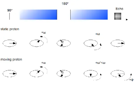
Using low diffusion-weighting values (b) DWI reduces DWI sensitivity to physiological motion but permits only the imaging of intravoxel incoherent motion (IVIM), which combines both water diffusion and perfusion. This work evaluates the context of low b-values DWI imaging of the human heart, proposes methodological contributions and then applies the developed techniques experimentally. Images acquisition is optimized on several parameters and an ideal time-window for robust cardiac triggering is defined. Eventual results of a dedicated acquisition strategy combined with image processing: PCATMIP-low b-values DWI, show significant improvements towards the application of cardiac DWI. Preliminary in vivo results encourage further clinical investigations and scientific developments.

(3)

JURY COMPOSITION:

Referees: David FIRMIN PhD

Jacques FELBLINGER PhD Jean-Nicolas DACHER MD, PhD

Invited: Virginie CALLOT PhD

Isabelle MAGNIN PhD

Yue-Min ZHU PhD

Directors: Pierre CROISILLE MD, PhD Denis GRENIER PhD

(4)

Résumé

L’Imagerie par Résonance Magnétique pondérée en Diffusion (IRM-D) permet l’accès à l’information structurelle des tissus au travers de la lecture du mouvement brownien des molécules d’eau. Ses applications sont nombreuses en imagerie cérébrale, tant en milieu clinique qu’en recherche. Néanmoins le mouvement physiologique créé une perte de signal supplémentaire au cours de l’encodage de la diffusion. Cette perte de signal liée au mouvement limite les applications de l’IRM-D quant à l’imagerie cardiaque. L’utilisation de faibles valeurs de pondération (b) réduit cette sensibilité mais permet seulement l’imagerie du mouvement incohérent intra-voxel (IVIM) qui contient la circulation sanguine et la diffusion des molécules d’eau. L’imagerie IVIM possède pourtant de nombreuses applications en IRM de l’abdomen, depuis la caractérisation tissulaire à la quantification de la perfusion, mais reste inexplorée pour l’imagerie du cœur.

Mon travail de thèse correspond à l’évaluation des conditions d’application de l’IRM-D à faibles valeurs de b pour le cœur humain, afin de proposer des contributions méthodologiques et d’appliquer les techniques développées expérimentalement.

Nous avons identifié le mouvement cardiaque comme une des sources majeures de perte de signal. Bien que la mouvement global puisse être corrigé par un recalage non-rigide, la perte de signal induite par le mouvement perdure et empêche l’analyse précise par IRM-D du myocarde. L’étude de cette perte de signal chez un volontaire a fournit une fenêtre temporelle durable où le mouvement cardiaque est au minimum en diastole. Au sein de cette fenêtre optimale, la fluctuation de l’intensité atteste d’un mouvement variable résiduel. Une solution de répéter les acquisitions avec un déclenchement décalé dans le temps permet la capture des minimas du mouvement, c.-à-d. des maximas d’intensité en IRM-D. La projection du maximum d’intensité dans le temps (TMIP) permet ensuite de récupérer des images pondérées en diffusion avec un minimum de perte de signal lié au mouvement.

Nous avons développé et évalué différentes séquences d’acquisition combinées avec TMIP : la séquence d’imagerie écho-planaire classique par écho de spin (SE-EPI) peut être adaptée mais souffre du repliement d’image ; une séquence Carr-Purcell-Meiboom-Gill combinée avec une préparation d’encodage de diffusion est plus robuste aux distorsions spatiales mais des artefacts de bandes noires empêchent son applicabilité ; finalement une séquence double-SE-EPI compensant les courants de Foucault et pleinement optimisée produit des images IRM-D moins artefactées. Avec cette séquence,

(8)

l’IRM-D-TMIP permet la réduction significative de la perte de signal liée au mouvement pour l’imagerie cardiaque pondérée en diffusion. L’inconvénient avec TMIP vient de l’amplification du bruit positif d’intensité.

Afin de compenser cette sensibilité du TMIP, nous séparons le bruit d’intensité des fluctuations lentes liées au mouvement grâce à une nouvelle approche basée sur l’analyse en composantes principales (PCA). La décomposition préserve les détails anatomiques tout en augmentant les rapports signal et contraste-à-bruit (SNR, CNR). Avec l’IRM-D-PCATMIP, nous augmentons à la fois l’intensité finale et la qualité d’image (SNR) en théorie et expérimentalement. Les bénéfices ont été quantifiés en simulation avant d’être validés sur des volontaires. De plus la technique a montré des résultats reproductibles sur des patients post-infarctus aigue du myocarde, avec un contraste cohérent avec la position et l’étendue de la zone pathologique.

Contrairement à l’imagerie cérébrale, l’imagerie IRM-D par faibles valeurs de pondération in vivo doit être différentiée des analyses IRM-D ex-vivo. Ainsi l’IRM-D-PCATMIP offre une technique sans injection pour l’exploration du myocarde par imagerie IVIM. Les premiers résultats sont encourageants pour envisager l’application sur un model expérimental d’une maladie cardiovasculaire. Enfin l’accès à des valeurs plus élevées de b permettrait l’étude du modèle complet IVIM du cœur humain, afin de séparer et quantifier à la fois la perfusion et la diffusion au sein des tissus.

(9)

Abstract

Diffusion weighted magnetic resonance imaging (DW-MRI, or DWI) enables the access to the structural information of body tissues through the reading of water molecules Brownian motion. Its applications are many in brain imaging, from clinical practice to research. However physiological motion induces an additional signal-loss when diffusion encoding is applied. This motion-induced signal-loss limits greatly its applications in cardiac imaging. Using low diffusion-weighting values (b) DWI reduces this sensitivity but permits only the imaging of intravoxel incoherent motion (IVIM), which combines both water diffusion and perfusion. IVIM imaging has many applications in body MRI, from tissue characterization to perfusion quantification but remains unexplored for the imaging of the heart.

The purpose of this work was to evaluate the context of low b-values DWI imaging of the heart, propose methodological contributions and then apply the developed techniques experimentally.

We identified cardiac motion as one of the major sources of motion-induced signal loss. Although bulk motion can be corrected with a non-rigid registration algorithm, additional signal-loss remains uncorrected for and prevents accurate DWI of the myocardium. The study of diffusion-weighted signal-loss induced by cardiac motion in a volunteer provided a time-window when motion is at minimum in diastole. Within this optimal time-window, fluctuation of intensity attests of variable remaining physiological motion. A solution to repeat acquisition with shifted trigger-times ease the capture of motion amplitude minima, i.e. DWI-intensity maxima. Temporal maximum intensity projection (TMIP) finally retrieves diffusion weighted images of minimal motion-induced signal-loss.

We evaluated various attempts of sequence development with TMIP: usual spin-echo echo-planar imaging (se-EPI) sequence can be improved but suffers aliasing issues; a balanced steady-state free-precession (b-SSFP) combined with a diffusion preparation is more robust to spatial distortions but typical banding artifacts prevent its applicability; finally a state-of-the-art double-spin-echo EPI sequence produces less artifacted DWI results. With this sequence, TMIP-DWI proves to significantly reduce motion-induced signal-loss in the imaging of the myocardium. The drawback with TMIP comes from noise spikes that can easily be highlighted.

To compensate for TMIP noise sensitivity, we separated noise spikes from smooth fluctuation of intensity using a novel approach based on localized principal component analysis (PCA). The decomposition was made so as to preserve anatomical features while increasing signal and contrast to

(10)

noise ratios (SNR, CNR). With PCATMIP-DWI, both signal-intensity and SNR are increased theoretically and experimentally. Benefits were quantified in a simulation before being validated in volunteers. Additionally the technique showed reproducible results in a sample of acute myocardial infarction (AMI) patients, with a contrast matching the extent and location of the injured area.

Contrarily to brain imaging, in vivo low b-values DWI should be differentiated from ex vivo DWI pure diffusion measurements. Thus PCATMIP-DWI might provide an injection-free technique for exploring cardiac IVIM imaging. Early results encourage the exploration of PCATMIP-DWI in an experimental model of cardiac diseases. Moreover the access to higher b values would permit the study of the full IVIM model for the human heart that retrieves and separates both perfusion and diffusion information.

Keywords: diffusion weighted imaging (DWI); cardiac magnetic resonance (CMR); intravoxel

incoherent motion (IVIM) imaging; temporal maximum intensity projection (TMIP); principal component analysis (PCA)

(11)

1. Introduction

The heart is a key organ in the human body. Cardiovascular diseases impact deeply the whole body, threatening all organs via the circulation system. Therefore cardiac imaging is a major discipline of radiology.

Magnetic resonance imaging (MRI) is a powerful mean to explore the human body non-invasively. Cardiac magnetic resonance (CMR) plays a major role in everyday patients’ care by diagnosing, preventing and following cardiac diseases non-invasively and without radiations.

Diffusion weighted magnetic resonance imaging (DW-MRI, or DWI) enables the access to the structural information of body tissues through the reading of water molecules Brownian motion. Its applications are many in brain imaging, from clinical practice to research. However when physiological motion occurs during diffusion encoding, an additional signal loss appears that limits the accuracy of DWI and bias results. This motion-induced signal-loss limits greatly its applications in cardiac imaging. A solution to reduce this sensitivity is to use low diffusion-weighting values (b) DWI. But low b-values DWI permits only the imaging of intravoxel incoherent motion (IVIM), which combines both water diffusion and perfusion. IVIM imaging has many applications in body MRI, from tissue characterization to perfusion quantification but remains unexplored for the imaging of the heart.

My work has been to define the context of feasibility for low b-values cardiac DWI in order to propose methodological contributions that could improve the reliability of cardiac DWI and/or ease the application of DWI in vivo. The purpose was to work in tight collaboration with the application towards possible immediate results in vivo.

This dissertation presents first the basis of cardiac imaging, then focuses on MRI technique, and especially describes DW-MRI. Once theoretical knowledge is stated, the developments and achievements of my thesis are exposed with the care of concision and clarity.

(12)

1.1. Clinical cardiac imaging: today’s challenges

Improving imaging of the heart is a necessity

The heart is one of the vital organs of the human body. Therefore its slightest defect might greatly

impact the whole body health. Thus cardiac imaging is critical in diagnosis procedures and this topic is a subject of intense research and investments.

1.1.1. Major public health issues and common pathologies

Cardiovascular diseases are the leading cause of death worldwide, making it a major public health

issue. Coronary heart disease was the world leading cause of death in 2004 with 7.2 millions of deaths, which represents 12.2% of overall deaths. Chronic cardiovascular diseases impacts particularly high-income countries. Ischemic cardiomyopathy alone, when oxygen supply to the heart is critically reduced, was responsible for 8% (~40 000 cases) of deaths in France in 2006, and all circulation diseases account for the second cause of death (28%) after tumors (30%){source: INSEE, CépiDc-Inserm }.

The increasing mortality rate related to cardiovascular death leads to growing interest and investments from governments in the topic. Major risks of cardiovascular disease come from new life style in wealthy countries and the same behavior in developing countries is becoming an important public health concern. Increased stress, too rich diet and reduced physical activity are reasons for increasing risk of heart failure and vascular pathology. Therefore investments go to both research and prevention, in order to improve health care as well as raise public awareness.

1.1.2. Cardiac imaging: purpose and techniques

Cardiac imaging stands as one of the top priorities towards improving health care, to provide better

and more accessible care to the numerous cardiovascular patients. Cardiac imaging is required to

provide accurate diagnosis as well as tools for treatments evaluation.

1.1.2.1. Diagnosis

Imaging is at the core of identification, diagnosis and follow-up for all major cardiovascular diseases today. While biomarkers enables the detection of abnormality and triggers disease suspicions, imaging

(13)

helps pathology detection and treatment choice. Accurate diagnosis helps to define treatments targets and guides chirurgical intervention.

Moreover imaging is a key to provide the follow-up to assess treatment efficiency. Subsequent treatment adjustments rely heavily on the radiologists’ conclusion.

Finally imaging also helps in new treatments evaluation, particularly for the heart which is difficult to access and analyze in vivo.

1.1.2.2. Prognosis

Aging as well as long-term diseases such as diabetes and obesity can impact severely the vascular system, including the heart. The mechanisms behind the complications are not always well understood and certainly not easy to anticipate. Cardiac imaging has an important role of prognostic to play in the

detection and the prevention of such complications before trauma occurs. Many other diseases or

dangerous genetic background are potential sources of future trauma and require regular check-ups. Accurate assessment of the current state of the body health in its deep foundations, especially the heart and the circulatory system, is needed to develop an efficient prevention.

1.1.3. Techniques: advantages and limitations

Cardiac imaging is giving a lot of interests towards many different applications. However imaging the heart is difficult and encounters many limitations. Investigating the heart can be done through 4 main imaging techniques, each with its own advantages and drawbacks: Positron emission Tomography (PET), very specific but suffers low resolution and exposes patients to radiations; Ultrasounds, easily accessible and non-invasive, but can image only a limited depth and with relative quality; Cone-beam X-ray

tomography (CT), which has a very good resolution but is difficulty specific and exposes patients to small

radiations; Magnetic Resonance Imaging (MRI) which offers a good resolution and specificity totally non-invasively but suffers a limited accessibility, related to its important cost.

Magnetic resonance imaging (MRI) has several advantages such as being harmless and non-invasive

and providing a wide range of information that enables the differentiations of many cardiac diseases. However MRI has the drawback of being expensive and is also one of the most complex medical imaging techniques actually used. Nuclear spins manipulation and subsequent signal detection works in the frequency space and a Fourier transform is needed to retrieve images spatial features. Therefore MRI development requires specific techniques implying combined state-of-the art mathematics and physics.

(14)

Although the first MR images were acquired 40 years ago, the complexity of an MR imaging acquisition process qualify it as a new imaging modality with a vast evolution potential and new breakthroughs are observed every year. The resolution and image quality is satisfactory although not as good as CT image quality. Finally MRI allows a wide variety of image contrasts that characterize tissues on variable basis so that many diagnosis can be performed (protons density, nuclear spins properties, etc) from a single MRI examination, with no harm for the patient. This access to different contrasts makes MR Imaging a technique of great potential in diagnosis for the cardiac muscle. Several contrast agents can also be employed in MRI: coated gadolinium (Gd) is the common one used to perform perfusion imaging but also ultra-small super-paramagnetic iron oxide (USPIO) are used as contrast agent in MRI. Gadolinium is coated because of its high toxicity if injected as is. Cardiac imaging benefits greatly from this contrast-enhanced imaging as it can determine the precise 3D localization and extent of an injury subsequent to a heart attack. Moreover MRI can access information from several nuclei. Common MRI is based on 1H resonance (water and organic tissues possess many 1_{H), but}31_{P MR spectroscopy (MRS) or}17_{O MRI are}

also interesting nuclei since 31_{P-MRS can measure myocardial adenosine triphosphate (ATP) and}

phosphocreatine (PCr) (Bottomley et Weiss 1998) and 17_{O MRI might able the quantification of oxygen}

consumption (McCommis et al. 2010). Thus MRI might enable to quantify the physiological tissues cells activity.

Among all imaging techniques, the choice to use one over the others is made depending on their diagnosis potential regarding suspected pathology but advantages and drawbacks like cost and accessibility are also taken in consideration and sometimes prevent any choice at all. This work focuses on cardiac MRI since many techniques are being developed in this field and benefit each other from their innovations (Lustig, Donoho, et Pauly 2007). Cardiac MRI is indeed a hot topic that currently motivates researchers worldwide.

(15)

1.2. Heart physiology

1.2.1. Introduction

To better understand the problematic of this thesis work, some basic knowledge of the cardiac physiology might be useful. This part is designed only for the basic understanding of the cardiac structure and function and focuses on their implication in the application of diffusion weighted magnetic resonance imaging to study the cardiac muscle.

1.2.2. Role of the heart

It might be obvious to some, but the heart plays a major role in the body system by circulating the blood from the lungs to the organs and backwards. The function of the heart acts as a double pump, propelling the deoxygenated blood to the lungs, where it is re-oxygenated, and then propelling the oxygenated blood towards all organs and tissues in the body (including the heart itself).

Figure 1: Blood circulatory system. The blood transports oxygen (in red) from the lungs, through the heart and to the body cells. Then the deoxygenated blood (blue) brings back carbon dioxide through the heart to the lungs to be expelled. Adapted from www.biosbcc.net .

(16)

1.2.3. Macroscopic heart anatomy

The human heart is about the size of a big fist and weights normally 250 to 350g. The heart functions as a double pump, decomposed in 4 cavities, with 4 valves separating each compartment:

• The atria: the right atria and the left atria, pre-chambers where flow is gathered • The ventricles: the right ventricle and the left ventricle, where flow is propelled.

The two ventricles are separated by the septum wall. On each side, the valves function by pairs to open and close the entry and exit points of blood flow. When a chamber is full, the entry valve closes and the exit valve opens. When the chamber needs refill, the exit valve closes and the entry valve opens. The valves are controlled by the ventricles contraction through chordae tendineae (orange) taking roots in papillary muscles (small muscles in grey).

Figure 2: Heart anatomy focus. Abbreviations are: RA, right atria; LA, left atria; RV, right ventricle; LV left ventricle; T, tricuspid valve; P, pulmonic valve; A, aortic valve; M, mitral valve.

The two sides are very different as the right ventricle propels the deoxygenated blood to the lungs, very close to the heart and easy to access, while the left ventricle propels the oxygenated blood to all the organs, requiring a lot of strength. Therefore the left ventricle muscle is usually thicker than the right ventricle.

(17)

The heart muscle consists of a continuum (Streeter et al. 1970) that can be described with three adjacent layers: the epicardium, the thin outer layer (<1mm), the myocardium, the middle layer (~7-9mm) and the endocardium, the thin inner layer (<1mm).

Figure 3: Heart wall muscles: from the exterior (epicardium) to the interior wall (endocardium). http://library.thinkquest.org/C003758/Structure/walls.htm

1.2.4. The cardiac cycle

The cardiac cycle can be decomposed in 4 steps. The focus is usually brought on the left ventricle, more critical than the right ventricle since it expels blood to the body, feeding the organs with oxygenated blood. But the two sides, the two ventricles function simultaneously.

Figure 4: Cardiac cycle description. Reproduced from www.cvphysiology.com

The four basic cardiac phases are:

a. Ventricular filling. The mitral valve is open. The ventricle dilates to fill blood in. (diastole)

b. Isovolumetric contraction. The mitral valve closes, the aortic valve remains closed. The ventricle contracts to increase the pressure in the ventricle.

(18)

c. Ejection. The aortic valve opens. The blood is ejected through the aorta to the body organs. d. Isovolumetric relaxation. The aortic valve closes. The myocardium relaxes the pressure in the

ventricle.

The cardiac cycle is usually simplified in two parts: the systole, active part of the cycle, includes phases b to d, and the diastole, passive part, the phase a where the blood filling dilates the relaxed myocardium. The cycle is accessible through its electrical activity that surface electrodes can capture. The reference being the strong R-wave corresponding to the trigger of the myocardium contraction (phase b). Most cardiac studies use the R-wave as the reference of time.

Figure 5: Electrocardiogram (ECG) and corresponding left ventricular pressure (LVP) and volume (LVV). Reproduced from www.cvphysiology.com

1.2.5. The myocardium microstructure

The cardiac muscle, the myocardium, is a very particular muscle in the human body that is a striated muscle as skeletal muscles, but involuntarily (contractile) as smooth muscles (e.g. autonomic nervous system of the eye).

There are three major types of cardiac cells (www.brown.edu):

• Cardiomyocytes - These are the cells that make up the contractile cardiac muscle. The cardiomyocytes are multinuclear such as cells in skeletal muscles (and contrarily to smooth muscles).

• Vascular endothelial cells - These cells are located in the inner lining of the heart blood vessels. They reduce turbulence of the flow of blood allowing the fluid to be pumped farther. They

(19)

regulate blood flow through vasoconstriction and vasodilation. They also act as a selective barrier that controls molecules transit through capillary membranes.

• Smooth muscle cells - These are located in the wall of the heart's blood vessels. They control the volume of blood vessels and the local blood pressure.

Figure 6: Histological section taken along the myocytes length. The fibrous arrays of myocytes with their multi-nucleus (dark spots) are seen. Reproduced from Wikipedia.org

The myocardium is composed of almost 80% of water, distributed among 3 main fluids compartments of interest appear (Bassingthwaighte, Yipintsoi, et Harvey 1974):

• Intracellular space, dense with cell activity, is where chemical reactions occur. Intracellular fluid makes up approximately 75-78% of myocardium water (Friedrich 2010) in healthy state. Intracellular water is tightly bound inside cells to proteins, ribonucleic acids and other molecules (see below for details).

• Interstitial space, part of extracellular space, is the space that carries all compounds between cells and the capillary system. Interstitial water accounts for 15-18% of myocardial water. Interstitial fluids are continually moving, being refreshed and recollected by lymphatic channels. Interstitial water moves slowly, driven by myocardial contraction and pressure gradients (mechanical pressure from intravascular space towards interstitium; osmotic pressure from K+/Na+ pump mechanisms to transit from intracellular space towards the venous system) (Mehlhorn et al. 2001).

• Intravascular space is the space inside the vascular circulatory system. Together with interstitial space, extracellular space makes up approximately 6-8 % of body water. Intravascular water is flowing at variable velocity (depending on the level of blood flow) and is slowly filtered through the endothelial barrier.

(20)

Figure 7: Model for water compartments in the myocardium. Intracellular space holds most of water in the myocardium and exchange easily water molecules with interstitial space in the healthy state. However water exchanges are limited through the

endothelial barrier between interstitial space and intravascular space.(Judd, Reeder, et May-Newman 1999)

Water molecules move rapidly through myocytes membrane between interstitial space and intracellular space. Water transits through cell membrane via 3 main routes: (1) by diffusion, (2) coupled to ion-channels or substrate transporters, such as glucose, Na+, K+ and Ca+, (3) via aquaporins, proteins that enable selective rapid transit in response to osmotic gradients(Egan et al. 2006). Indeed like water, ions, proteins and molecules rapid exchanges in and out cells are required to supply metabolic mechanisms that provide for cellular function and energy (ATP). Among these mechanisms, ionic pumps (Na+, K+, Ca+ and H+) are critical to the control of metabolic regulation and osmotic gradients. As a part of this transit control, ionic pumps also regulate most of intracellular water content and water molecules displacements between intra and extracellular spaces.

Additionally intracellular water possesses a particular diffusion pattern in the myocardium since cardiomyocytes are elongated cells composed of bundled proteins filaments (Figure 8). Thus water molecules diffusion is tightly constrained spatially but in the longitudinal direction of myocytes. Additionally cardiomyocytes are well aligned to form fibers (myofibers), thus water moves preferably in one main direction that defines locally the microstructure of the myocardium.

(21)

Figure 8: Ultrastructure of the working myocardial cell. Contractile proteins are arranged in a regular array of thick and thin filaments (seen in cross section at left). The A-band represents the region of the sarcomere occupied by the thick filaments, whereas the I-band is occupied only by thin filaments that extend toward the center of the sarcomere from the Z-lines, which bisect each I-band. The sarcomere, the functional unit of the contractile apparatus, is defined as the region between two Z-lines, and so contains two half I-bands and one A-band. The sarcoplasmic reticulum, an internal membrane system, consists of the sarcotubular network at the center of the sarcomere and the subsarcolemmal cisternae; the latter form composite structures with the transverse tubular system (t-tubules) and the sarcolemma called dyads. The t-tubular membrane is continuous with the sarcolemma, so that the lumen of the t-tubules carries the extracellular space toward the center of the myocardial cell. Mitochondria are shown in the central sarcomere and in cross section at the left.(Katz 2005; Topol et al. 2002)

Therefore intracellular and interstitial water molecules displacements occur locally along one main direction: the direction of myofibers. Additionally capillaries are aligned to this fibers structure, so

that cardiac microcirculation follows the same direction (Callot et al. 2003). Consequently both diffusion and perfusion follows a pattern specific to the myocardium architecture (detailed further down in 1.2.7.). The displacement freedom of fluids within each compartment is a major parameter of tissue health.

Accessing the quantity of water molecules for each compartment and the microscopic motion of molecules (molecules diffusion and flow) is a critical mean to diagnosing tissues’ health.

1.2.6. The coronary flow mechanics (Rossi 2007)

The heart has a unique perfusion sequence. Because of the cardiac muscle contraction the vascular system is squeezed during systole. Thus contrarily to other organs, coronary perfusion mostly occurs during diastole.

Coronary blood flow is unique in the sense that it occurs on and into the heart which is alternately contracting and relaxing. Thus the phasic nature of blood flow into and through its muscular wall is a little different from other organs. As a consequence of that, in contrast to all other organs, coronary arterial blood flow occurs predominantly during diastole. Coronary arterial blood flow at rest is low

(22)

during systole, and then increases markedly in early diastole. Then it falls off in parallel with aortic

pressure during mid-to-late diastole, and then falls abruptly during isometric ventricular contraction, prior to aortic valve opening. The reverse occurs with coronary venous blood flow which is high during systole and low during diastole. These cyclic changes are less marked in the right coronary arteries, supplying predominantly the right ventricle, but are very marked in the left coronary artery, which supplies the left ventricle.

Figure 9: Left anterior descending coronary pressure (P) and blood flow velocity (U) for a healthy 62y.o. woman.(Siebes et al. 2009)

Therefore, although coronary perfusion is needed to sustain myocardial contraction, the latter seems to be an impeding factor for coronary perfusion. It is as if left ventricular contraction squeezes branches of the coronary arteries entering the myocardium so that nearly no flow can occur through these vessels during systole. The small amount of blood flowing into the left coronary artery during systole probably just dilates the epicardial branches of this artery (DOUGLAS et GREENFIELD 1970; Hoffman et Chilian 2000; F W Prinzen et al. 1985; Freeman et al. 1985). During diastole, squeezing ceases with myocardial relaxation and the coronary system of the left ventricle is perfused by the pressure gradient between origin − aorta, and exit − right atrium.

Additionally the myocardium requires a constant supply of oxygen to function. Whereas body muscles can sustain certain duration in anaerobic state, the myocardium cannot sustain local oxygen privation longer than 20-40 min without irreversible necrosis. Therefore compared to other organs, capillary density in myocardium is high (3-4 .103_{capillaries per mm² cross section) and effective}

(23)

1.2.7. The myocardium global architecture

As mentioned above, cardiac tissues are made of myocytes aligned into myofibers. The myofibers organize themselves into sheets. Global heart’s architecture is positioned as a helix of muscle fibers that enhance the contraction mechanisms to increase the blood propeller-then-suction power. The fibers layers rotate across the myocardium wall with a progressive angle (from -90° to 90°(Wu et al. 2006)) to create the helix. In this configuration, the shortening of fibers amplifies the compression of the left ventricular cavity. This architecture is critical to the pump function of the heart. The alteration of this structure, such as in the process of remodeling after infarction (Wu et al. 2009; Streeter et al. 1970) can weaken the cardiac function.

Figure 10: Fibers orientation in the heart. Left: The myocardial “grain” as seen at various depths through the left ventricular wall of the porcine heart, visualized by peeling aggregates of myocytes stepwise in planes intruding from the epicardium to the endocardium. Note the turn of the grain upon a radial axis (red arrows). PA shows the origin of the pulmonary trunk from the right ventricle. LV, left ventricle. Right: the cartoon shows the variation in angle of the long axis of the myocytes aggregates when assessed relative to the ventricular equator. This is the so-called helical angle.(Anderson et al. 2006)

Conclusion

Overall the cardiac muscle possesses a complex architecture and a unique functional behavior among body organs. The heart function is critical to other organs. Consequently cardiac diseases deeply affect their viability. The prevention as well as the diagnosis of cardiovascular pathologies is a topic of intense research, especially throughout developments of cardiac imaging.

(24)

1.3. MRI

Quantum physics - harmless body tissues exploration

Here is proposed a brief overview of nuclear magnetic resonance (NMR) with the classic model in order for the reader to reach faster the core of this thesis contribution. The author does realize the limitations of this model and is aware of risky but necessary shortcuts made in the following text, and asks talented quantum physics experts’ forgiveness in order for them to focus on his accomplishments.

1.3.1. NMR principles

Nuclear Magnetic Resonance (NMR) is based on the interaction between an exterior magnetic field and particles’ nuclear spins. Spin is a quantum fundamental property of particles. It can be represented as equivalent to an inner rotating magnetic momentum, and is determined by 2 parameters: its spin quantum number s (as every fundamental property, it is discrete: s=0,±1/2, ±1) and its direction described by a vector.

• Electrons, neutrons and protons (1_{H) have a spin s=1/2}

• Photons have a spin s=1 Proton NMR: basis

Let us now consider 1H atoms, with s=1/2 corresponding spin. An externally applied magnetic field Bo applied to a proton population will have 2 effects:

1. Their spins will start oscillating around the field axis at a pulsation proportional to the field strength: ω=γBo. This is the Larmor precession.

(25)

It is possible to show the rotation is limited to a cone, with a given cone angle θm≈54.74°.

2. Their energy levels split. This is the Zeeman effect (Zeeman 1897).

The splitting occurs because of the interaction of the magnetic moment µ of the atom with the magnetic field B slightly shifts the energy of the atomic levels by an amount:

𝛿𝐸 = −µ. 𝑩 (I.)

This energy shift depends on the relative orientation of the magnetic moment and the magnetic field{Physics 387 Home Page}. The magnetic momentum of the proton is:

µ = 𝑔𝑒. 𝑰 2𝑚= 𝛾𝑰

(II.)

Given the proton’s charge e and its mass m. g is a dimensionless factor(the g-factor), gH≈ 5.586. And

γ is the gyromagnetic ratio, characteristic for each nuclide (γ= γ/2π=42.577 MHz/T for 1_{H). Resulting}

(26)

𝛿𝐸 = ±µ𝑧𝐵𝑜 = ±𝑔

𝑒. ℏ

4𝑚. 𝐵𝑜= ±𝛾𝑠ℏ𝐵𝑜= ±ℏ𝑠𝑣

(III.)

The energy gap between the two population is then ΔE=-2δE=-hγB=-hv, with v corresponding frequency. The difference in populations between those two energy levels can be expressed with the Boltzmann statistics, with a naturally larger population for the lower energy level (thus the minus in the formula above):

𝑎 =𝑁 + 𝑁 −= 𝑒

−Δ𝐸_𝑘𝑇 (IV.)

Considering protons in a human body (T=37°C) within a clinical magnetic resonance imaging magnet of B=1.5T, we obtain v=63.87 MHz and a=1.000009882611, that is a difference of n=(a-1)/(a+1)=4.94ppm(part-per-million), which is a really small difference!

Because of this very small spins population difference, NMR signal is usually very weak and a strong magnetic field is required in order to capture a significant signal.

Also since the human body is composed of a lot of water, and water molecules possess two protons (H2O), nuclear magnetic resonance of the proton is the most effective non-invasive NMR method to study body tissues.

Am I hearing resonance?

It is possible to make spins “hop” between populations by applying an electromagnetic radiofrequency (RF) pulse of the same energy as the gap between the two energy levels. The system will absorb the RF pulse energy, perturbing its equilibrium state, then it will return progressively to its initial state while restituting part of the given energy. This is the nuclear magnetic resonance (NMR).

In order to match corresponding energy difference, the RF pulse is calibrated on a frequency basis with the Larmor frequency connecting energy and frequency: vo= ωo/2π =-γB, as seen above.

(27)

The two levels of energy can be represented (quantum probabilities apart) with the spins: the lower level corresponds to spins z-components aligned parallel to the external magnetic field while the higher level corresponds to spins aligned anti-parallel to the external field.

Figure 11: The difference in spins populations creates a macroscopic magnetic momentum M.

In a static external magnetic field Bo, a resulting magnetic moment M is created by the sum of unbalanced spin momentum, align parallel to the magnetic field. Applying RF pulses will enable the manipulation of this magnetic momentum M, from flipping it into transverse plane relative to static Bo, to flipping it entirely along the longitudinal axis(=Bo axis).

NMR corresponds to the excitation-relaxation-reception of the magnetization M with varying parameters that enables the characterization of the sample.

1.3.2. NMR experiment

As seen previously, the excitation RF pulse is a variable electromagnetic field B1 rotating around the

Bo axis at the Larmor pulsation ωo. Considering the frame turning with the spins at ωo, the Larmor

pulsation, the RF pulse can be represented as an additional fixed magnetic field B1 in a classic mechanic

model. Applying this field in the transverse plane, here on x-axis, creates a torque T on M according to the Laplace force:

𝑻 = 𝑴 × 𝑩𝟏= 1 γ d𝑴 dt → d𝑴 dt = 𝑴 × γ𝑩𝟏 (V.)

(28)

Figure 12: Rotation of macroscopic magnetization subject to a local radio-frequency variable electromagnetic field B1.

The RF pulse leads to the rotation of the M vector around B1 axis (x-axis) with a speed equal to

ω1=γB1. Eventual rotation angle is 𝜃 = ∫ 𝛾𝐵₁(𝑡)𝑑𝑡

𝑡𝑖𝑚𝑝

given timp the RF impulsion time. NMR RF pulses

are usually characterized by this rotation angle 𝜃, ranging from 0 to 180°(full flip of magnetization M), with common value at 90°(flip of M into the transverse plane,then Mz=0).

At resonance, the magnetization simply rotates around B1 in the rotating frame of reference,

while in the laboratory frame the motion of M is a spiral (nutation) caused by the precession around the vector sum of B0 and B1(t).

Figure 13: Excitation (left) and relaxation (Right) of the macroscopic magnetization. The relaxation occurs in a spiral trajectory that rotates (=nutation) around the intense static field Bo.

Relaxation of the magnetization (Absil 2006)

After being excited, the spins system returns to its thermal equilibrium state in the field Bo, this is the spin-latice relaxation (T1). The magnetization during relaxation is ruled by the Bloch equations

(Bloch 1946). The excited magnetization presents a second relaxation time, the transverse (spin-spin) relaxation time, depending on spins phasing/dephasing during the nutation:

(29)

• The longitudinal relaxation («spin-lattice» relaxation) is due to energy exchanges with the surrounding lattice. Actually, the spin system transfers the energy given by the excitation and tends to come back to the difference of energy level population at thermal equilibrium (more spins on the lowest state).

𝑀𝑧(𝑡) − 𝑀𝑜 = (𝑀𝑧(𝑡𝑜) − 𝑀𝑜)𝑒−𝑡−𝑡𝑜𝑇1 (VI.)

The longitudinal relaxation is characterized by the relaxation time T1. Any NMR experiment has

to consider T1 since it conditions the time allowed to the magnetization to recovers from previous

excitation before doing the next excitation. Therefore the repetition time (TR) choosen is related to the

T1 of the sample.

• The transverse relaxation («spin-spin» relaxation) is due to interactions between the spins themselves. These interactions progressively and irreversibly dephase the spins in the transverse plane, leading to a decay of the transverse macroscopic magnetization toward zero.

𝑀𝑥𝑦(𝑡) = 𝑀𝑥𝑦(𝑡𝑜) 𝑒−𝑡−𝑡𝑜𝑇2 (VII.)

The transverse relaxation is characterized by the relaxation time T2. Note that the transverse

magnetization decreases faster than the longitudinal magnetization, therefore T2<T1. In the case

of short T2, the sequence needs to be fast otherwise the signal intensity is too small to be

captured. The echo time (TE) needs to be much smaller (conventionally five time) than the T2

of the sample (50-100ms).

With the proton density ρ, these two relaxation times T1 and T2 are the most common

parameters used to modulate the image contrast of a MR Imaging experiment, ,. These 3 parameters are the primary characteristics of tissues characterization in nuclear Magnetic Resonance Imaging (MRI).

1.3.2. MRI techniques: signal formation

The excitation as well as the signal detection is performed with coils based on the Faraday’s law of induction. Inducing an electrical current in a transmitting coil generates a magnetic field. Reversely the variation of the magnetic flux through the coil surface generates an electrical current.

(30)

Figure 14: Basis of NMR excitation-reception. Excitation: an alternative current in the coil generates a variable magnetic field on the spin lattice. Reception: the magnetization generates a variable flux that induces electrical currents in the coil.

The electrical signal received by a receiving coil is called the Free Induction Decay (FID). This is an alternative signal oscillating around the Larmor frequency.

Spin Echo techniques

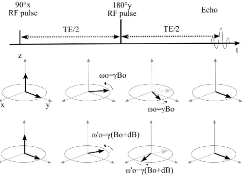
In order to “read” the magnetization, M is rotated into the transverse plane, manipulated with variable magnetic fields: magnetic gradient then brought back to its initial angle in the transverse plane. This creates an echo, appearing at a specific chosen time: the echo time TE. One the most common NMR sequence proceeds as follow:

-A 90° RF pulse along the x axis at t=0

-A 180° RF pulse along the y axis at t=TE/2

(31)

Figure 15: Spin echo principle. The spin echo enables to refocus spins even in the case of static magnetic field

inhomogeneities (case at the bottom). Echo time (TE) occurs at twice the elapsed time between the excitation and the refocusing pulse (TE/2).

The advantage of such a method appears when we consider inhomogeneities in the static magnetic field Bo. The spins precess at different frequencies depending on their location in the inhomogeneous magnetic field. But with the spin echo scheme, they are all rephrased at the echo time.

Spin echo NMR sequences have the advantage of being able to compensate for Bo inhomogeneities.

Spin echo sequences have:

• Less sensitivity to magnetic field inhomogeneity

• Higher SAR since at least 2 RF pulses are required one being a 180° pulse • Longer TE, that affects motion sensitivity and T2 signal decrease

The present work in this manuscript will make use of a spin echo MRI sequence.

Gradient Echo techniques

In order to “read” the magnetization, M is rotated by only a small angle (𝛼) from the longitudinal axis (z). Magnetic gradients rotate the magnetization back then forth to bring it back to its initial position. This creates an echo in the rotating frame (at 𝜔 = 𝛾𝐵0), appearing at a specific chosen time:

(32)

-A 𝛼° RF pulse (here along the x axis at t=0)

-A gradient lobe of intensity -G, along the readout direction, of duration 𝜏

- A gradient lobe of intensity +G, along the readout direction, of duration 2𝜏

Gradient echo techniques are:

• Very fast (short TE)

• Use less RF power, thus deposit less energy in the body (low SAR).

• Are sensitive to magnetic field inhomogeneities. Spins at different magnetic field strength will not be refocused identically, thus the echo intensity will be less than for a spin echo at same TE.

The present work in this manuscript will not make use of a gradient echo MRI sequence in this form.

Balanced Steady-State Free Precession (b-SSFP) techniques

Balanced-SSFP mechanism was described long ago (Carr 1958), but has become of interest only through more recent developments which provide a robust T2/T1 contrast technique. Balanced-SSFP is

(33)

Figure 16: Schematic construction of a balanced-Steady State Free Precession (b-SSFP) MR sequence. The combination of a spin echo and a gradient echo creates a steady state after the second RF pulse (+𝛼°𝑥) that can be maintained with repeated RF

pulses.

After the initial half-spin echo, the pattern in gray dashed-square is repeated for each line. At echo time (TE), both a spin echo from previous pulses and a gradient echo from present gradients are superimposed. Thus the repeat time TR=2*TE.

The technique is fast, with high echo intensity, but suffers off-resonance artifacts from its magnetic field inhomogeneity sensitivity, like gradient echo techniques. The present work in this manuscript will make use of a b-SSFP MRI sequence.

1.3.3. MRI: Encoding spatial information

Now that we know how to characterize tissues with NMR, it is important to be able to localize the source of the signal to differentiate tissues. All localization is based on the Larmor frequency relationship.

Basic space encoding scheme

1. The first step is to image only one slice using a space-selective excitation. The slice selection is performed with adding a linear gradient Gs to the static field Bo along its direction (z-axis) during excitation. Thus the magnetic field the spins see depends on their z position, so does their resonance frequency:

𝜔𝑂(𝑧) = 𝛾(𝐵𝑜 + 𝑑𝐵(𝑧)) (VIII.)

By applying this gradient, it is possible to excite only spins within a defined slice thickness Δz with a corresponding selective excitation frequency bandwidth of Δω=(γGs)*Δz.

(34)

Figure 17: MRI slice selection principle. A magnetic gradient G creates a linear relationship between the magnetic field B and the spins location along the axis z: B(z). Thus spins resonance frequency depends on z according to the Larmor equation. Finally only the spins whose frequency is within range of excitation pulse frequency are excited: only a slice along axis z is excited.

2. Once a slice has been selected, the acquisition of the image remains to be done. Positional information along a first dimension is obtained by modifying magnetizations’ phases along one of the inplane directions (in the example along the y-axis). This is the phase encoding step. By applying a linear gradient Gφ (as in step 1.) during a time t along the y-axis, the transverse magnetizations undergo different precession frequencies depending on their location along this axis. Therefore, at the end of the phase encoding step, different magnetizations along the y-axis have acquired different phase angles F which are function of their y-position. Thus lines can be resolved by reading the magnetization phase after application of the phase gradient.

𝑦 =𝜙(𝑦)

𝛾𝐺𝜙𝜏 (IX.)

3. The final step is to resolve voxels within each line. As in step 1, a linear gradient Gω is used on the x direction during the readout of the signal. Thus spins frequency depend on their location along the x-axis. This is the frequency encoding step.

𝑥 =𝜔(𝑥) 𝛾𝐺𝜔

(35)

Figure 18: MRI spatial encoding. First is the selective slice excitation with a gradient across the slice Gss. Then is the line encoding with a phase-gradient Gφ. Finally is the frequency encoding gradient Gω during the readout of the echo that differentiate voxels along each line. Corresponding time diagram for a spin-echo MRI experiment is illustrated on the right panel (Kastler et al. 2006).

With this the location of each voxel is determined by its phase (=line on y-axis) and its frequency (=column on x-axis) at the time of readout. This creates the so-called k-space which presents 2 axis: phase and frequency axis. In order to recover the image from this k-space, a 2D Fourier transform is applied to convert phase-frequency information into spatial x-y information.

Image reconstruction

Since MRI signal is acquired in the phase-frequency domain, a (discrete) 2D-Fourier transform (FT) is necessary to retrieve spatial information (since phase-frequency information is discrete within a pixels matrix, a discrete 2D-FT is used).

𝑆(𝑥, 𝑦, 𝑡) = ∑ ∑ 𝐾(𝑥, 𝑦, 𝑡). 𝑒𝑗(𝜔(𝑥)𝑡+𝜙(𝑦))

𝑥 𝑦

(XI.)

Where K(x,y,t) represents the magnetization measured in k-space (phase-frequency space) and

S(x,y,t) the spatial magnetization in the image space.

Low frequencies, corresponding to greatest changes in the image (contrast) are in center of k-space, while high frequencies, corresponding to small feature, details in the image, are in the outer k-space.

(36)

Figure 19: Image reconstruction depends on k-space content. Low-frequency k-space corresponds to contrast; High-frequency k-space corresponds to details in the image.

Echo Planar Imaging(EPI)

The basic space encoding scheme as described previously present a major flaw as it requires repeating the whole sequence for each encoded line desired. But it is possible to acquired the full k-space within one “shot” by successively dephase(change line) and read one line. This technique is called

echo planar imaging. But since signal decays in time because of T1 and T2 relaxations, the EPI scheme

was designed to read the whole k-space as fast as possible. Therefore gradient times are minimized by reading lines alternatively back and forth.

(37)

Figure 20: Time-diagram of an Echo Planar Imaging (EPI)MRI spin-echo sequence. Corresponding lines letters are reported on the read k-space on the right panel(DeLaPaz 1994).

This technique remains subject to improvements every year because of its sensibility to gradients flaws. It assumes ideal linear gradients while real gradients are subject to amplitude fluctuation and their switching time might be longer than predicted. It also remains limited in speed because of the gradients max amplitude and slew rate (see. 1.2.1. Gradients).

However the work presented in this manuscript depends only on EPI technique, with simple improvements such as partial k-space acquisition, sampling during gradients establishment (ramp-sampling, this is sampling while the practical linear gradients are not yet fully established) and post-processing distortions correction. With these improvements, EPI is a fast imaging technique that is more robust to off-resonance artifacts than some faster techniques such as spiral imaging(highly sensitive in cardiac imaging). Off-resonance artifacts come from an unexpected shift of resonance frequency. Different tissues in the body create additional gradients to the magnetic field. These static susceptibility effects cause the signal to appear at the “wrong” frequency. Other sources of off-resonance effects can be eddy currents. The effect of off-resonance with EPI is a signal loss and geometrical distortions, usually a shift in the image that does not affect the interpretation. However other fast readout techniques such as spiral are highly sensitive to off-resonance effects, which manifest as a damageable blurring. Therefore EPI remains a good compromise for fast MRI.

1.3.4. MRI hardware

Magnetic resonance imaging (MRI) implies several technological choices as well as many limitations depending on the study of interest. This part proposes a simplified overview of the main hardware elements needed to acquire an MR image:

(38)

• A strong static magnetic field usually provided by a superconducting magnet of several Teslas to create the magnetization. This magnet is coupled to a battery of “shims” (adjustable magnetic coils used to insure the best field homogeneity within the magnet.

• Radio frequency (RF) magnetic field emitting coils. These coils are needed to “create” a detectable magnetization (kW) to create the detectable signal

• RF magnetic field receiving coils. These coils are needed to acquire the macroscopic MR signal (mW) to detect the macroscopic signal.

• Spatially varying magnetic fields able to switch at audio frequency speed (gradients). • And a computer to reconstruct images.

Each of these elements are vitals for the image MR images synthesis process and have to be dimensioned according to the MRI purpose (generic, cardiology, neurology, spectroscopy, imaging, ….)

Figure 21: NMR experiment simple interactions model. The excitation creates a NMR signal, which can be influenced by magnetic field gradients and/or RF pulses. Resulting NMR signal is captured by a receiving coil. Excitation and reception coils can

be differentiated or the same coil can play both roles. Bo Magnet

Nuclear Magnetic Resonance occurs only in an intense static magnetic field. The main component of a MRI system is the magnet. The NMR signal increases with the static magnetic field strength, suggesting that higher fields are more suited for MRI (Haacke et al. 1999):

𝑆𝑖𝑔𝑛𝑎𝑙 ∝ 𝛾

3_𝐵𝑜3_𝜌

𝑇

(39)

Apart from the technical difficulty of creating a stable magnet of great intensity, increasing the magnetic field presents several issues to the experimentation in vivo. High field technical challenges

include (Snyder et al. 2009):

• field in-homogeneity

• sub-optimal ECG performance

Another immediate consequence of increasing the magnetic field strength is the increased difficulty to acquire electrophysiological activity, especially electro cardiogram (ECG) gating. The magneto-hydrodynamic effects cause the magnetic field to induce electrical currents in moving conductive fluid, modifying the magnetic field itself, but also spoiling the ECG. Synchronization is complicated at high fields (see figure below of ECG at 1.5T and 7T).

Figure 22: Electro-cardiogram (ECG) for 0.5 and 7T. ECG distortions increase within high magnetic fields. Triggering becomes an issue for such intense fields NMR experiments on humans. (Snyder et al. 2009)

For all these reasons, clinical magnets are limited in magnetic field strength at 1.5 and more recently

3 Tesla.

RF pulses

A stronger static field implies the use of higher frequency RF pulses, which provides higher NMR signal but images become more sensitive to field variations. Magnetic field in-homogeneity introduces greater artifacts in the images. Motion, pulsation and susceptibility effects such as tissues interfaces (esp. air-tissues interfaces) are all sources of magnetic field inhomogeneity, creating as many sources of

(40)

The main reason to limit magnetic field strength also comes from the consequently increasing radiofrequency power deposition on the patient’s body that creates an important heating of the tissues. The mechanism for heating is the induction of eddy currents in the body by the time-dependent RF magnetic field in accordance with Faraday’s Law, due to the finite conductivity of the body. Absorption of RF power by the tissue is described in terms of Specific Absorption Rate (SAR), which is expressed in W/kg. (In the US, the recommended SAR level for head imaging is 3.2 Watts/kg.) SAR in MRI is a function of many variables including RF pulses frequency (related to field strength), pulse sequence, coil parameters and the weight of the region exposed. Because the proportion of power absorbed by the tissues is very high (70 to 90%), calibration of RF pulses is primordial.

Figure 23: Power and SAR measurements from the prototype SAR dosimeter. The measured output power from the RF amplifier (blue diamonds and line of best fit), the measured input power to the birdcage coil (incident minus reflected power; green squares and line), and the total power deposited in the transducer as deduced from Eq. [1] (cyan crosses and line), all as a function of the power measured on the dosimeter load RL on the horizontal axis. The cyan curve relating actual-to-measured power in the dosimeter, is used for calibration. The red line (red triangles) plot the SAR (vertical axis at right) for the average head in W/kg, as a function of the power measured in RL on the horizontal axis. [A Prototype RF Dosimeter for Independent Measurement of the Average Specific Absorption Rate (SAR) During MRI](Stralka et Bottomley 2007)

While MRI would benefit higher resonance signal from increased excitation power, the SAR estimation and regulation provides the limits of application both in instantaneous power deposition and long-term heating during the full examination. Cardiac imaging is deeply affected by SAR limitation as the excitation needs to input a sufficient power amount into the heart muscle which in buried in the thorax, sometimes through a big wall of flesh, bones and fat. A lot of power is absorbed in the way, and the compromise between the minimum power to obtain a good enough image and the maximum power the

(41)

SAR limit can tolerate for the thorax. The calibration of RF excitation is usually done by the scanner,

which probes the “sample” before any MR exam. The MRI software estimates in real time the amount of energy deposit in the patient and prevent any armful heating by stopping the sequence acquisition or preventing it’s launching if the energy deposit becomes higher than a safety threshold.

For all these reasons, clinical magnets are commonly limited in magnetic field strength at 1.5 and

more recently 3 Tesla.

Gradients

Spatial manipulation of the magnetization is done through the use rapidly varying magnetic field gradients. Gradients, which are switched on and off and modified during the course of the imaging experiment, have many uses, including:

• dephasing or refocusing magnetization • Selective excitation

• Spatial encoding

• Contrast creation (such as perfusion and diffusion imaging) Gradients are characterized by 3 parameters:

• Their amplitude • Their duration • Their rise time

The stronger gradients the hardware can achieve, the shorter the Echo Time and the better the spatial resolution can be. Also the shorter time the gradients are applied, the faster the images can be acquired, increasing the time resolution of examination. However the variation of the magnetic field causes the induction of electrical currents within body tissues. Thus their use has several limitations, both in speed and intensity. Typical maximum gradient amplitude in clinical scanners reaches 40 to 80

(42)

amplitude, either positive or negative. The slew rate is based on both the hardware limits and the limitation imposed by the induction in the body. Typical slew rate ranges 100 - 200 mT/m/msec.

Once all the hardware has been dimensioned, the sequence design implies different combinations of gradients and RF pulses towards the contrast desired. The more accurate and robust the contrast researched is, the more demanding on hardware the sequence will be. That is especially true in the case of diffusion weighted MRI contrast that aims at water molecule Brownian motion at a microscopic level.

1.4. Diffusion Weighted Magnetic Resonance Imaging (DW-MRI or

DWI)

Non-invasive exploration of tissues structure

Basic MRI contrast characteristics were described previously: T1, T2 and proton density 𝜌. This paragraph will focus on another contrast, one that is of interest for this work: diffusion weighted MRI.

1.4.1. Diffusion theory

Brownian motion, or diffusion, describes the thermal random motion particles in a fluid undergo. This is a stochastic process in which particles probability density function associated to the position of the particles follows Brownian statistics. In our case, this is the random motion from water molecules in body tissues. Reading the diffusion of water molecules enables to characterize tissues as the random walk of molecules is restricted by their environment that is tissues structure. Therefore diffusion imaging has been of high interest in the past decade and remains yet a major subject of study and development.

In molecular diffusion, the moving entities are small molecules, here water molecules. They move at random because they frequently collide. Since collision times in typical solvents like water are about 0.1 nanoseconds, it is not possible to access microscopic motion with magnetic resonance imaging; however it is possible to access the macroscopic displacement of water molecules. Since diffusion is a three dimensional phenomenon, the mean displacement can be measured in every direction of space. The mean-square displacement <r²> depends on the time of observation t and the characteristic diffusion coefficient D (in m²/s). D is the diffusion coefficient that, according to Fick’s law,