Probabilistic models in physics, biology and actuarial science.

HAL Id: tel-02915245

https://tel.archives-ouvertes.fr/tel-02915245

Submitted on 13 Aug 2020

HAL is a multi-disciplinary open access

archive for the deposit and dissemination of sci-entific research documents, whether they are pub-lished or not. The documents may come from teaching and research institutions in France or abroad, or from public or private research centers.

L’archive ouverte pluridisciplinaire HAL, est destinée au dépôt et à la diffusion de documents scientifiques de niveau recherche, publiés ou non, émanant des établissements d’enseignement et de recherche français ou étrangers, des laboratoires publics ou privés.

science.

Hélène Guerin

To cite this version:

Hélène Guerin. Probabilistic models in physics, biology and actuarial science.. Probability [math.PR]. Université de Rennes 1 (UR1), 2019. �tel-02915245�

HABILITATION À DIRIGER

DES RECHERCHES DE

L’UNIVERSITE DE RENNES 1

COMUE UNIVERSITE BRETAGNE LOIRE

Ecole Doctorale N°601

Mathèmatique et Sciences et Technologies de l’Information et de la Communication Spécialité : (voir liste des spécialités)

Par

Hélène GUÉRIN

Comportement en temps long et étude de modèles probabilistes

pour des phénomènes physiques, biologiques et actuariels.

Unité de recherche : IRMAR - UMR CNRS 6625 Thèse N°:

Rapporteurs avant soutenance :

Arnaud GUILLIN, Professeur, Université Blaise Pascal Stéphane LOISEL, Professeur, Université Lyon 1 - ISFA Sylvie RŒLLY, Professeure, Universität Potsdam

Composition du jury :

Présidente : Eva LÖCHERBACH, Professeure, Univeristé Paris 1

Examinateurs : Jean-Christophe BRETON, Professeur, Université de Rennes 1 Loïc CHAUMONT, Professeur, Université d’Angers

Arnaud GUILLIN, Professeur, Université Blaise Pascal Stéphane LOISEL, Professeur, Université Lyon 1 - ISFA Sylvie RŒLLY, Professeure, Universität Potsdam

Contents

Remerciements 5

Introduction 7

1 Notations . . . 8

2 Some probabilistic tools . . . 9

2.1 The notion of infinitesimal generator of a Feller process . . . 9

2.2 Some distances in probability . . . 10

3 List of publications . . . 11

1 Transport Theory, Particle Systems Models in kinetic theory : the Boltzmann and Landau equations 13 1 The spatially homogeneous Boltzmann and Landau equations and their probabilistic representation . . . 14

1.1 The Boltzmann equation . . . 14

1.2 Probabilistic approach of the Boltzmann equation . . . 16

1.3 The Landau equation and its associated process . . . 17

2 Well-posedness of the spatially homogeneous Boltzmann equation . . . 19

2.1 Some notations . . . 20

2.2 Assumptions on the collision kernel . . . 21

2.3 The main results . . . 22

3 Well-posedness of the spatially homogeneous Landau equation . . . 23

3.1 Existing results and goals . . . 23

3.2 A general inequality . . . 24

3.3 Applications . . . 24

4 Mean field interacting particle system for the Landau type processes . . . . 24

4.1 An interacting particles system . . . 25

4.2 Convergence to the nonlinear Landau type process . . . 26

4.3 Mesurability of optimal transportation for a general cost . . . 28 3

2 Long time behavior of Piecewise Deterministic Markov Processes

A model in biology : chemotaxis of a flagellated bacterium 31

1 The model . . . 32

2 The reflected process . . . 36

3 Coalescent coupling for the reflected process . . . 36

3.1 Jump times of the reflected process . . . 37

3.2 A Coupling for the reflected processes . . . 39

3.3 Estimate of the speed of convergence to the equilibrium . . . 42

4 Convergence to equilibrium for the initial process . . . 44

5 To go further . . . 46

3 Markov Switching Processes, Spectrally Negative L´evy Processes Some actuarial and financial issues 49 1 Di↵usions with Markov switching . . . 50

1.1 Invariant measure of the di↵usion with Markov switching . . . 51

1.2 Intuition and scheme of the proof . . . 53

1.3 Speed of convergence to equilibrium . . . 57

2 Di↵erent notions of ruin in insurance . . . 57

2.1 Some models in insurance . . . 58

2.2 Some notions of ruin . . . 60

2.3 Other risk measures . . . 63

3 Occupation time of L´evy processes in finite time . . . 66

3.1 Joint distributions of occupations times and the process sampled at a fixed time . . . 67

3.2 Applications in finance and in insurance . . . 68

4 To go further . . . 71

Remerciements

De nombreuses personnes ont contribu´e, de pr`es ou de loin, math´ematiquement ou pas, `

a la r´ealisation du travail dont ce document est la synth`ese. Je souhaite ici leur t´emoigner toute ma reconnaissance.

Je souhaite tout d’abord remercier mes rapporteurs Arnaud Guillin, St´ephane Loisel et Sylvie Rœlly d’avoir accept´e de rapporter mon m´emoire d’habilitation `a diriger des recherches. J’en fus extrˆemement honor´ee car vous repr´esentez chacun `a votre mani`ere et chacun dans votre domaine l’excellence et le dynamisme scientifique. Je remercie aussi tr`es chaleureusement ´Eva L¨ocherbach, avec qui depuis nos premiers pas en recherche, nous ´evoluons chacune de notre cot´e, tout en se croisant r´eguli`erements, d’avoir accept´e de pr´esider mon jury de soutenance. Je souhaite enfin remercier Jean-Christophe Breton et Lo¨ıc Chaumont pour leur participation `a ce jury. Il ´etait vraiment important pour moi d’avoir votre regard scientifique sur mon travail. Si je devais mentionner un directeur pour ce m´emoire, le nom de Jean-Christophe me viendrait naturellement tellement il m’a accompagn´e et soutenu dans le processus de r´edaction.

Une personne ´etait malheureusement absente lors de cette journ´ee, principalement `a cause de ma mauvaise organisation, une personne qui m’est tr`es ch`ere. Sylvie M´el´eard m’a transmis le goˆut de la recherche, a pouss´e ma curiosit´e, tout en d´eveloppant ma rigueur scientifique. Mˆeme si depuis mon doctorat, nos th`emes de recherche se sont ´eloign´es, j’ai toujours grand plaisir `a la retrouver et poursuivre nos discussions scientifiques.

Les travaux pr´esent´es ici n’auraient pas ´et´e les mˆemes sans les rencontres stimulantes que j’ai fait depuis mon doctorat. Je remercie l’ensemble de mes collaborateurs avec qui j’ai eu ´enorm´ement plaisir `a discuter pour imbriquer nos id´ees sur des sujets fascinants. Les ´echanges que l’on peut avoir lors de collaborations restent pour moi le meilleur moteur pour la recherche. J’esp`ere que nous continuerons `a travailler ensemble sur de nouveaux projets.

Je souhaite bien ´evidemment remercier l’UFR de Math´ematiques de l’universit´e de Rennes 1 et l’Institut de Recherche Math´ematique de Rennes et leur personnel admin-istratif, pour le merveilleux cadre de travail qu’ils o↵rent `a leurs enseignants-chercheurs. C’est une vrai chance de pouvoir ´evoluer dans cet environnement stimulant et bienveillant. J’ai eu beaucoup de plaisir `a travailler au sein de l’´equipe Processus Stochastiques du pˆole al´eatoire de l’IRMAR. Je tiens `a saluer ici mes coll`egues, `a la fois pour nos ´echanges sci-entifiques et amicaux (parfois autour d’un bon repas pour certains) : Bernard, Guillaume, Isma¨el, Jean-Christophe, J¨urgen, Mihai, Nathalie, St´ephane, Ying,... Sans oublier les col-l`egues de la pause m´eridienne avec qui j’ai eu plaisir `a partager mon repas dans la petite cuisine de l’IRMAR : David, Guy, Goulwen, ´Eric,...

Il y a aussi bien entendu les anciens qui sont partis bien avant moi de Rennes : Jean-Baptiste Bardet, Florent Malrieu, Philippe Briand et Philippe Berthet. Je dois avouer parfois regretter l’ambiance bon enfant et dynamique de mes d´ebuts `a Rennes avec mes deux comp`eres Jean-Baptiste et Florent et leurs familles. J’ai par ailleurs une pens´ee pour mes coll`egues plus loin g´eographiquement : Joaquin Fontbona, Victor Rivero, Jean-Fran¸cois Renaud,...

Enfin, mes derniers mots s’adressent `a mes proches, `a ma famille. Je souhaite ici saluer le soutien ind´efectible d’Arthur, sa capacit´e `a prendre le relais et bien sur l’´energie sans limite de mes enfants : Ma¨el, Romane et Fleur.

Introduction

This document is an overview of my di↵erent works since my PhD thesis. I have consid-ered probabilistic models for di↵erent applications, in physics, biology or actuarial science, always with the aim of studying carefully the behavior and properties of the underlying process. Most of my results investigates the question of the long-time behavior of stochastic processes.

The first model I studied is about some rarefied homogeneous gas in kinetic theory. The behavior of the particles is given either by the well-known Boltzmann equation or by the Landau equation, depending on the nature of the collision between particles. During my thesis, I worked on the existence of solutions to the Landau equation by a probabilistic way, their regularity and on the link between the Boltzmann solutions and the Landau solutions. I continued to explore this subject during the first years after my PhD thesis. With Nicolas Fournier, we studied the dependence on the initial condition of the solutions of the Boltzmann and the Landau equation, [FG08, FG09]. With Joaquin Fontbona and Sylvie M´el´eard, we have been interested in constructing an easily simulable di↵usive inter-acting particle system converging towards the nonlinear Landau process and in obtaining an explicit speed of convergence, [FGM09, FGM10]. The results on the Boltzmann and Landau equations are presented in Chapter 1 of this document.

With Florent Malrieu and Joaquin Fontbona, we have been interested in the study of a model in biology, more precisely a model describing the behavior of a flagellated bacterium in its environment. The general model introduced by Erban and Othmer being quite com-plex with many parameters, we considered a simplified model in order to obtain interesting and quantitative results on the long time behavior of the bacterium using a probabilistic approach, [FGM12, FGM16]. The behavior of a such bacteria is modelized by a piecewise deterministic Markov process (PDMP). This kind of processes has been extensively stud-ied during the last decade, and can also have many applications, especially for e↵ective Monte-Carlo algorithms. Although we have considered a fairly simple model, the study of

its long time-behavior has highlighted the important role of jump times, especially when the deterministic flows are not contractive. Using a geometrical coupling, we obtained an explicit speed of convergence to equilibrium. These results are presented in Chapter 2 of this document.

During a long stay in Montr´eal in 2012-2014, I have met some researchers in actuar-ial science which led to fruitful collaborations in ruin theory for the spectrally negative L´evy framework, [BSGMF15, GR16, GR17]. We worked on new ruin measures, which ex-tend the classical probability to have a negative surplus in the case of spectrally negative L´evy model. We can relate those results to the work on Ornstein-Ulhenbeck di↵usions with Markov switching, in collaboration with Florent Malrieu and Jean-Baptiste Bardet, [BGM10], which has applications in finance and in insurance. The results related to these topics are presented in Chapter 3 of this document.

Each chapter of this work can be read independently from the others. In the next sections of this introduction, we give some common notations (the devoted notation of each chapter being defined therein), and we recall some well-known definitions and results in probability which will be used in di↵erent chapters of this document.

1

Notations

Let d 1. Let us denote by C₁2 Rd (resp. C_b2 Rd , resp. C_c2 Rd ) the set of C2-functions :Rd _{7! R of which the second derivative is bounded (resp. of which the derivatives of}

order 0 to 2 are bounded, resp. which are compactly supported). Let also Lp _Rd _{be the space of measurable functions f with}

kfkLp_(Rd_{) :=} ✓Z Rd fp(v) dv ◆1/p < +1. Let us introduce⇣⌦,_{F, (F}t)t 0,P ⌘

a filtered probability space. The distribution of a random variable X will be denoted by_L(X). Let P Rd _{be the set of probability measures onR}d_{, and for k 1,}

Pk ⇣ Rd⌘₌n_{f 2 P}⇣_Rd⌘_{, m} k(f ) <1 o with mk(f ) := Z Rd|v| k_{f (dv).}

We denote by L1 [0, T ],Pk Rd and L1 0, T ], Lp Rd the sets of measurable families

(ft)t2[0,T ]of probability measures onRdsuch that supt2[0,T ]mk(ft) <1,R₀T ||ft||Lpdt <1

respectively.

ID R+,Rd will denote the Skorohod space of c`adl`ag functions fromR+intoRd. This space

Finally we denote x^ y = min(x, y), x _ y = max(x, y) for x, y 2 R+, and z.˜z the scalar

product of z, ˜z_{2 R}dand Mt and M⇤ are respectively the transpose matrix and the adjoint matrix of the matrix M .

For some set A we write 1Athe usual indicator function of A.

2

Some probabilistic tools

We introduce in this section some classical probabilistic tools which are used throughout this document. Specific tools for each model will be introduced in the devoted chapter.

2.1 The notion of infinitesimal generator of a Feller process

Let (E,_{E) be a measurable space. On a filtered probability space (⌦, F, (F}t)t 0,P), we

consider (Xt)t 0a Feller process with transition (Pt)t 0with values in (E,E), which means

that X is a Markov process with transition (Pt)t 0, i.e. for any nonnegative measurable

function f and s < t,

E[f(Xt)|Fs] = Pt sf (Xs) P ps,

such that for any t 0, any continuous function f , Ptf is a continuous function and

limt#0Ptf (x) = f (x).

The infinitesimal generator of a Feller process X is the operator defined, for f a continuous function, by

Lf = lim

t#0

1

t(Ptf f ).

The domain D(L) of the operator L is the subset of continuous functions such that the previous limit exists.

Consequently, for f _{2 D(L),}

E[f(Xt+h) f (Xt)|Ft] = hLf (Xt) + o(h).

The operator L describes the infinitesimal behavior of the process on a small time interval. We can observe that if f _{2 D(L), the process Mt}f = f (Xt) f (X0) R₀tLf (Xs)ds is a

(Ft,P⌫) martingale for any initial measure ⌫, see [RY94].

A measure µ is said to be an invariant measure for the Markov process X if for any t 0,

any smooth function f , _Z

Ptf dµ =

Z f dµ,

or equivalently, _Z

2.2 Some distances in probability

The Wasserstein distance

Let us consider processes in dimension d 1.

For two probability measures µ, ⌫ 2 Pp Rd and ⇡ 2 Pp(Rd⇥ Rd), we write ⇡ <µ⌫ if the

marginals of ⇡ are ⇡1 = µ and ⇡2 = ⌫. The Wasserstein distanceWp on Pp Rd is defined

as follows: for any µ, ⌫ _{2 P}p(Rd),

Wp(µ, ⌫) = ✓ inf ⇡<µ⌫ ⇢Z |x y_|p⇡(dx, dy) ◆1/p (0.1) = infnE[|X Y |p] : (X, Y )_{2 R}d_{⇥ R}d random vectors with _{L(X) = µ and L(Y ) = ⌫}o1/p. It is well-known that _Pp Rd ,Wp is a complete metric space (see [Vil02]).

For p = 2,_W2 is called the Wasserstein distance with quadratic cost c(x, y) =|x y|2. The

topology endowed by the Wasserstein distance is stronger than the usual weak topology (for more details, see Villani, [Vil03] Theorem 7.12). It is well-known that the infimum is actually a minimum, and that if µ (or ⌫) has a density with respect to the Lebesgue measure onRd, then there is a unique ⇡ <µ⌫ such thatW22(µ, ⌫) =

R

Rd_⇥Rd|x y|2⇡(dx, dy).

In section 4.3 of Chapter 1, the question of optimal transportation for the Wasserstein distance with general costs will be considered.

The total variation distance

The total variation distance between two probability measures µ and ⌫ in some measurable space (_{X , B) is given by} kµ ⌫kTV= sup A2B{|µ(A) ⌫(A)|} = 1 2sup{|µ( ) ⌫( )| : k k1 1}. (0.2) We notice that

kµ ⌫kTV= inf{P(X 6= Y ) : X, Y random variables with L(X) = µ, L(Y ) = ⌫}, (0.3)

where each pair of random elements (X, Y ) of _{X is simultaneously constructed in some} probability space and is called a coupling. See [Lin92] for alternative definitions of this distance and its main properties.

Let us notice that the Wasserstein distance is quantitative while the total variation distance is qualitative. Indeed, the Wasserstein distance is small if there exists a coupling (X, Y ) with close random variables while this is not enough for the total variation distance. For example,

Wp( x, y) =|x y|, k x yk_TV= 1x6=y,

3

List of publications

[GR17] Gu´erin, H´el`ene; Renaud, Jean-Fran¸cois, On the distribution of cumulative Parisian ruin, Insurance Math. Econom., 73, 2017, 116–123

[FGM16] Fontbona, Joaquin; Gu´erin, H´el`ene; Malrieu, Florent, Long time behavior of telegraph processes under convex potentials, Stochastic Process. Appl., 126, 2016, 10, 3077– 3101

[GR16] Gu´erin, H´el`ene; Renaud, Jean-Fran¸cois, Joint distribution of a spectrally negative L´evy process and its occupation time, with step option pricing in view, Adv. in Appl. Probab., 48, 2016, 1, 274–297

[BSGMF15] Ben-Salah, Zied; Gu´erin, H´el`ene; Morales, Manuel; Firouzi, Hassan Omidi, On the depletion problem for an insurance risk process: new non-ruin quantities in collective risk theory, Eur. Actuar. J., 5, 2015, 2, 381–425

[FGM12] Fontbona, Joaquin; Gu´erin, H´el`ene; Malrieu, Florent, Quantitative estimates for the long-time behavior of an ergodic variant of the telegraph process, Adv. in Appl. Probab., 44, 2012, 4, 977–994

[BGM10] Bardet, Jean-Baptiste; Gu´erin, H´el`ene; Malrieu, Florent, Long time behavior of dif-fusions with Markov switching, ALEA Lat. Am. J. Probab. Math. Stat., 7, 2010, 151–170

[FGM10] Fontbona, Joaquin; Gu´erin, H´el`ene; M´el´eard, Sylvie, Measurability of optimal trans-portation and strong coupling of martingale measures, Electron. Commun. Probab., 15, 2010, 124–133

[BGM15] Bardet, Jean-Baptiste; Gu´erin, H´el`ene; Malrieu, Florent, On the Laplace transform of perpetuities with thin tails, arXiv: 0912.3232, 2009

[FG09] Fournier, Nicolas; Gu´erin, H´el`ene, Well-posedness of the spatially homogeneous Lan-dau equation for soft potentials, J. Funct. Anal., 256, 2009, 8, 2542–2560

[FGM09] Fontbona, Joaquin; Gu´erin, H´el`ene; M´el´eard, Sylvie, Measurability of optimal trans-portation and convergence rate for Landau type interacting particle systems, Probab. Theory Related Fields, 143, 2009, 3-4, 329–351

[FG08] Fournier, Nicolas; Gu´erin, H´el`ene, On the uniqueness for the spatially homogeneous Boltzmann equation with a strong angular singularity, J. Stat. Phys., 131, 2008, 4, 749–781

[GMN06] Gu´erin, H´el`ene; M´el´eard, Sylvie; Nualart, Eulalia, Estimates for the density of a nonlinear Landau process, J. Funct. Anal., 238, 2006, 2, 649–677

[Gu´e04] Gu´erin, H´el`ene, Pointwise convergence of Boltzmann solutions for grazing collisions in a Maxwell gas via a probabilistic interpretation, ESAIM Probab. Stat. 8, 2004, 36–55

[GM03a] Gu´erin, H´el`ene; M´el´eard, Sylvie, Convergence from Boltzmann to Landau processes with soft potential and particle approximations, J. Statist. Phys., 111, 2003, 3-4, 931–966

[Gu´e03] Gu´erin, H´el`ene, Solving Landau equation for some soft potentials through a proba-bilistic approach, Ann. Appl. Probab., 13, 2003, 2, 515–539

[Gu´e02] Gu´erin, H´el`ene, Existence and regularity of a weak function-solution for some Landau equations with a stochastic approach, Stochastic Process. Appl., 101, 2002, 2, 303– 325

Transport Theory, Particle

Systems

Models in kinetic theory : the

Boltzmann and Landau equations

My first steps in research concerned the study of the Bolzmann and Landau equations in kinetic theory by a probabilistic way. I continued to explore this topic during the first years after my PhD thesis. The results obtained during this period are presented in this chapter. With Nicolas Fournier, Sorbonne universit´e, we have studied the dependence on the initial condition of the solutions of the Boltzmann and of the Landau equations. These results has been published in Journal of Statistical Physics, On the uniqueness for the spatially homogeneous Boltzmann equation with a strong angular singularity, [FG08], and in Journal of Functional Analysis, Well-posedness of the spatially homogeneous Landau equation for soft potentials, [FG09].

With Joaquin Fontbona, Universidad de Chile, and Sylvie M´el´eard, CMAP, ´Ecole Poly-technique, we have been interested in constructing an easily simulable di↵usive interacting particle system converging towards the nonlinear Landau process and in obtaining an ex-plicit speed of convergence. These results rely on two articles, Measurability of optimal transportation and convergence rate for Landau type interacting particle systemspublished in Probability Theory and Related Fields, [FGM09], and Measurability of optimal trans-portation and strong coupling of martingale measures published in Electronic Communi-cations in Probability, [FGM10]. The approach was quite new and used in a sophisticated way the optimal transport theory.

Let us first introduce the spatially homogeneous Boltzmann and Landau equations.

1

The spatially homogeneous Boltzmann and Landau

equa-tions and their probabilistic representation

1.1 The Boltzmann equation

The spatially homogeneous Boltzmann equation is an important equation from kinetic theory which describes the evolution of the density ft(v) of particles with velocity v 2 R3

at time t in a rarefied homogeneous gas. This is a nonlinear di↵erential equation given by @f

@t = QB(f, f ), (1.1)

with QB the quadratic collision kernel defined by

QB(f, f )(t, v) = Z R3 dv_⇤ Z S2 d B(_|v v_{⇤|, ✓)}⇥ft(v0)ft(v_⇤0) ft(v)ft(v⇤)⇤

where the pre-collisional velocities are given by v0 = v + v⇤ 2 + |v v_⇤| 2 , v 0 ⇤ = v + v_⇤ 2 |v v_⇤| 2 , (1.2)

and ✓ is the so-called deviation angle defined by cos ✓ = (v v⇤)

|v v⇤| · . The collision kernel

B(_{|v v⇤|, ✓) = B(|v}0 v_⇤0_{|, ✓) depends on the nature of the interactions between particles.} This equation is quite natural: it says that for each v _{2 R}3, new particles with velocity v appear due to a collision between two particles with velocities v0 and v0_⇤, at rate B(_|v0 v_⇤0|, ✓), while particles with velocity v disappear because they collide with another particle with velocity v_⇤, at rate B(_{|v v⇤|, ✓). See Desvillettes [Des01] and Villani [Vil02] for more} details.

Since the collisions are assumed to be elastic, conservation of mass, momentum and kinetic energy hold at least formally for solutions to (1.1), that is for all t 0,

Z R3 ft(v) (v) dv = Z R3 f0(v) (v) dv, for (v) = 1, v,|v|2.

We classically assume without loss of generality thatR_R3f0(v) dv = 1.

We also assume that for some functions :R+ 7! R+ and : (0, ⇡]7! (0, 1), the collision

kernel is of the form

B(_|v v_{⇤|, ✓) sin ✓ = (|v} v_{⇤|) (✓).} (A1)

When particles interact through repulsive forces in 1/rs, with s _{2 (2, 1), one has (see} Cercignani [Cer88]) (z) = z , (✓)_⇠ 0 cst ✓ 1 ⌫_{, with =} s 5 s 1 2 ( 3, 1), ⌫ = 2 s 1 2 (0, 2). One classically names hard potentials the case when 2 (0, 1) (i.e., s > 5), Maxwellian molecules the case when = 0 (i.e., s = 5), moderately soft potentials the case when 2 ( 1, 0) (i.e., s 2 (3, 5)), and very soft potentials the case when 2 ( 3, 1) (i.e., s2 (2, 3)).

In any cases, R₀₊ (✓)d✓ = +_{1, which expresses the a✏uence of grazing collisions, that} is collisions with a very small deviation. We will assume here the general physically rea-sonnable conditions Z ⇡ 0 (✓)d✓ = +_{1, }1 := Z ⇡ 0 ✓2 (✓)d✓ < +_1. (A2)

Let us define the notion of weak solutions we shall use.

Definition 1.1. Let B be a collision kernel which satisfies (A1-A2). A family f = (ft)t2[0,T ]2 L1([0, T ],P2(R3)) is a weak solution to (1.1) if Z T 0 dt Z R3 ft(dv) Z R3 ft(dv⇤) (|v v⇤|) |v v⇤|2 < +1, (1.5)

and if for any 2 C2 1 R3 , and any t2 [0, T ], Z R3 (v) ft(dv) = Z R3 (v) f0(dv) + Z t 0 ds Z R3 fs(dv) Z R3 fs(dv⇤)A (v, v⇤), (1.6) where A (v, v⇤) = (|v₂ v⇤|) Z ⇡ 0 (✓)d✓ Z 2⇡ 0 d'⇥ (v0) + (v0_⇤) (v) (v_⇤)⇤.

As noted by Villani [Vil98b, p 291], one has, for all v, v_{⇤2 R}3, all ✓_{2 [0, ⇡], all 2 C1}2 R3 , Z 2⇡

0

d'⇥ (v0) + (v_⇤0) (v) (v_⇤)⇤ _{ C||} 00_||1✓2_|v v_⇤|2,

so that thanks to assumption (A2), (1.5) ensures that all the terms in (1.6) are well-defined. Let us now introduce the jump amplitude

a := a(v, v_⇤, ✓, ') := (v0 v) = (v_⇤0 v_⇤). (1.7) One of the main difficulties of this equation is that a is not a Lipschitz continuous function on the variables v and v_⇤. It just satisfies an “almost”-Lipschitz property of a (Lipschitz up to a rotation), as proved in [Tan79] or in its “fine” version in [FM02].

1.2 Probabilistic approach of the Boltzmann equation

Since R₀⇡✓ (✓)d✓ may be infinite and taking into account the conservation of the mass, we introduce the following definition of probability measure solutions of (1.1).

Definition 1.2. We say that a probability measure family (Qt)t 0 is a measure-solution of

the Boltzmann equation (1.1) if for each 2 C2 b(R3) Z (v)Qt(dv) = Z (v)Q0(dv) + Z t 0 ZZ K _, (v, v_⇤)Qs(dv) Qs(dv⇤) ds, (1.8)

where K _, is defined in the compensated form by K _, (v, v_⇤) = b (v v_⇤)(v v_⇤)._{r (v)} + Z 2⇡ 0 Z ⇡ 0 ✓ (v + a(v, v_⇤, ✓, ')) (v) a(v, v_⇤, ✓, ')._{r (v)} ◆ (_|v v_{⇤|) (✓)d✓d'} and where b = ⇡ Z ⇡ 0 (1 cos ✓) (✓)d✓.

We can consider (1.8) as the evolution equation for the marginals of a Markov process whose law is defined by a martingale problem. Indeed, the distribution Q can be seen as the law of a stochastic process belonging to ID(_R+,R3) solution of the nonlinear stochastic

di↵erential equation Vt= V0 b Z t 0 Z R3 (_|Vs z|)(Vs z)Qs(dz)ds + Z t 0 Z R3 Z R+ Z ⇡ 0 Z 2⇡ 0 a(Vs , z, ✓, ')1{x (|Vs z|)}N˜⇤(dx, d✓, d', dz, ds)

where ˜N⇤ is the compensated martingale of an inhomogeneous Poisson-point measure on R+⇥[0, ⇡]⇥[0, 2⇡]⇥R3⇥R+with intensity dx (✓)d✓d'Qt(dz)dt. The nonlinearity appears

through Qs, which is the law of Vs for each s.

We consider a compensated form of the Poisson-point measure following Definition 1.2. That gives a pathwise mean-field interacting representation of the Boltzmann process: the process jumps following a Poisson-point measure which picks independent colliding partic-ules having the same law as the process itself. The jump takes place if x (|Vs z|)

and the amplitude of the jump is equal to a.

1.3 The Landau equation and its associated process

The Landau equation is a continuous approximation of the Boltzmann equation: when there are infinitely many infinitesimally small collisions, the particle velocities become continuous in time. The most interesting case is that of Coulomb potential (i.e. when = 3), since then the Boltzmann equation seems to be meaningless. It is also the most difficult case to study mathematically. However, the Landau equation can be derived from the Boltzmann equation with very soft potentials, that is 2 ( 3, 1) (see see Funaki [Fun85], Goudon [Gou97], Villani [Vil98b, Vil98a] and Gu´erin-M´el´eard [GM03b, Gu´e04]). The main idea is that the more is negative, the more the Landau equation is physically interesting. We refer to [Vil02] for a detailed survey about such considerations.

Consequently, the Landau equation, also called the Fokker-Planck-Landau equation, de-scribes the collisions of particles in a plasma and is obtained as limit of Boltzmann equations when the grazing collisions prevail. In the spatially homogeneous case, it writes in IR3:

@f @t = QL(f, f ) (1.9) with QL(f, f ) (t, v) = 1 2 3 X i,j=1 @ @vi ⇢Z IR3dv⇤Aij(v v⇤)  ft(v⇤) @ft @vj (v) ft(v) @ft @v_⇤j (v⇤)

where ft(v) 0 is the density of particles having velocity v 2 IR3 at time t 2 IR+, and

(Aij(z))_1i,j3 is a nonnegative symmetric matrix depending on the interaction between

the particles, of the form

A (z) =_|z| +2⇧ (z) =_|z| 2 4 z 2 2 + z23 z1z2 z1z3 z1z2 z12+ z32 z2z3 z1z3 z2z3 z21+ z22 3 5 (1.10)

where ⇧ (z) is the orthogonal projection on (z)? and _{2 ( 3, 0] the potential. As A is a} symmetric nonnegative matrix, there exists a matrix such that A = . ⇤_{, where is the}

adjoint matrix of . There is not uniqueness of .

Like for the Boltzmann equation, we observe that the solutions to (1.9) conserve, at least formally, the mass, the momentum and the kinetic energy: for any t 0,

Z R3 ft(v) (v)dv = Z R3 f0(v) (v)dv, for (v) = 1, v,|v|2.

We classically may assume without loss of generality that R_R3f0(v)dv = 1. Another

fun-dammental a priori estimate is the decay of entropy, that is solutions satisfy, at least formally, for all t 0,

Z R3 ft(v) log ft(v)dv Z R3 f0(v) log f0(v)dv.

By integration by parts, see [Vil98b], a weak formulation of Equation (1.9) writes, at least formally, for any test function 2 C2

b IR3 , d dt Z R3 (v)ft(v)dv = ZZ R3_⇥R3 ft(dv)ft(dv⇤)L (v, v⇤) (1.11)

where the operator L is defined by L (v, v⇤) = 1 2 3 X i,j=1 Aij(v v⇤)@ij2 (v) + 3 X i=1 bi(v v⇤)@i (v) (1.12) with bi(z) = 3 X j=1 @jAij(z) = 2|z| zi, for i = 1, 2, 3. (1.13)

Let us mention that existence of weak solutions, under physically reasonnable assumptions on initial conditions, has been obtained by Villani [Vil98b].

Like for the Boltzmann equation, using the conservation of mass, we introduce a definition of probability-measure solutions of the Landau equation :

Definition 1.3. Let P0 belong to P2 IR3 . A weak solution of the Landau equation (1.14)

with initial data f0 is a family (ft)t 0 of probability measures in P2 R3 satisfying

Z (v) ft(dv) = Z (v) f0(dv) + Z t 0 ZZ L (v, v_⇤) fs(dv) fs(dv⇤) ds (1.14)

for any function _{2 Cb}2 IR3 where L is the Landau kernel defined by (1.12).

The probability measure solution of the Landau equation can be seen as the distribution of a Markov processes X of a nonlinear stochastic di↵erential equation of type:

Xt= X0+ Z t 0 Z R3 (Xs y)WP(dy, ds) + Z t 0 Z R3 b(Xs y)Ps(dy)ds (1.15)

where is a ”square-root” of the matrix A defined by (1.10), b is defined by (1.13), Ptis the

law of Xt, and WP is aR3 valued space-time white noise on [0, T ]⇥ R3 with independent

coordinates, each of which having covariance measure Pt(dy)⌦ dt, in the sense of Walsh

[Wal86].

The nonlinear process (1.15) was introduced by Funaki [Fun84], who obtained existence and uniqueness results for Lipschitz coefficients :R3 ! R3⌦3 _{and b :R}3 _{! R}3_{, see also}

Gu´erin [Gu´e02, Gu´e03] for a di↵erent approach.

2

Well-posedness of the spatially homogeneous Boltzmann

equation

We investigate in this section the question of the well-posedness of the spatially homoge-neous Boltzmann equation for singular collision kernel as introduced above. In particular we are interested in uniqueness and stability with respect to the initial condition.

In the case of a collision kernel with angular cuto↵, that is when R₀⇡ (✓)d✓ < +_{1, there} are some optimal existence and uniqueness results: see Mischler-Wennberg [MW99] and Lu-Mouhot [LM12].

The case of collision kernels without cuto↵ is much more difficult, but is very important, since it corresponds to the previously described physical collision kernels. This difficulty is not surprising: on each compact time interval, each particle collides with infinitely (resp. finitely) many others in the case without (resp. with) cuto↵.

In all the previously cited physical situations, global existence of weak solutions has been proved by Villani [Vil98b] by using some compactness methods.

Tanaka [Tan79], Horowitz-Karandikar [HK90], Toscani-Villani [TV99] studied uniqueness for non cuto↵ collision kernel in the case of Maxwellian molecules: it was proved in [TV99] that uniqueness holds for the Boltzmann equation as soon as is constant and (A2) is met,

for any initial (measure) datum with finite mass and energy, that isR_R3(1 +|v|2) f0(dv) <

+_1.

Then there has been three papers in the case where is non cuto↵ and is not con-stant. The case where is bounded (together with additionnal regularity assumptions) was treated in [Fou06], for essentially any initial (measure) datum such thatR_Rd(1+|v|)f0(dv) <

1. More realistic collision kernels have been treated by Desvillettes-Mouhot [DM09] and Fournier-Mouhot [FM09] (including hard and moderately soft potentials). However, all these results apply only when assuming the following condition, stronger than (A2),

Z ⇡ 0

✓ (✓)d✓ <1. (1.16)

In particular, this does not apply to very soft potentials ( 2 ( 3, 1]). Weighted Sobolev spaces were used in [DM09], while the results of [FM09] rely on the Kantorovich-Rubinstein distance.

With Nicolas Fournier in [FG08], we obtained the first uniqueness result which can deal with the case where only (A2) is supposed. Our result is based on the use of the Wasserstein distance with quadratic cost. The main interest of our paper concerns very soft potentials, for which we obtain the uniqueness of the solution provided it remains in Lp(R3), for some p large enough. Since we are only able to propagate locally such a property, we obtain some local (in time) well-posedness result.

Our method could be applied to the case of hard potentials, but we have not treat this case, since there are already some available uniqueness results, as said previously.

Our proof is probabilistic, and we did not manage to rewrite it in an analytic way. The main idea is quite simple: for two solutions (ft)t 0, ( ˜ft)t 0 to the Boltzmann equation, we

construct two stochastic processes (Vt)t 0 and ( ˜Vt)t 0 whose time marginal laws are given

by (ft)t 0 and ( ˜ft)t 0, and which are coupled in such a way that E[|Vt V˜t|2] is “small” for

all times. This bounds from above the Wasserstein distance with quadratic cost between ft and ˜ft.

2.1 Some notations

For ↵2 ( 3, 0), we introduce the space J↵ of probability measures f on R3 such that

J↵(f ) := sup v2R3

Z

R3|v

v_⇤|↵f (dv_⇤) <1, (1.17)

We denote by L1 [0, T ],_Pk , L1 [0, T ], Lp , L1([0, T ],J↵) the set of measurable families

(ft)t2[0,T ]of probability measures onR3such that supt2[0,T ]mk(ft) <1,

RT

0 ||ft||Lpdt <1,

RT

Remark 1.4. For ↵ 2 ( 3, 0) and p > 3/(3 + ↵), there exists a constant C↵,p > 0 such

that for all nonnegative measurable f :R3 _{7! R, any v}⇤ _{2 R}d J↵(f ) ||f||L1 + C_↵,p||f||_Lp.

For a nonnegative function f _{2 L}1_(R3_{), we denote its entropy by}

H(f ) = Z

R3

f (v) log(f (v))dv.

2.2 Assumptions on the collision kernel

We now introduce, for ✓2 (0, ⇡], H(✓) :=

Z ⇡ ✓

(x)dx and G(z) := H 1(z).

Here H is a continuous decreasing bijection from (0, ⇡] into [0, +1), and its inverse function G : [0, +_{1) 7! (0, ⇡] is defined by G(H(✓)) = ✓, and H(G(z)) = z. We will suppose that} there exists 2> 0 such that for all x, y2 R+,

Z ₁

0

(G(z/x) G(z/y))2dz_{ }2

(x y)2

x + y . (A3)

Concerning the velocity part of the cross section, we will assume that for all x, y2 R+,

min(x2, y2)[ (x) (y)]

2

(x) + (y) + (x y)

2_{[ (x) + (y)]}

+ min(x, y)|x y|| (x) (y)|  (x y)2[ (x) + (y)] for some function :R+ 7! R+, with for some 2 ( 3, 0], some 3 > 0, for all x2 R+,

(x)_{ }3x . (A4( ))

Under Assumption ((A4)( )), we can easily see that necessarily for all x _{2 R}+, (x) 

(x), and then (x)_{ }3x .

These assumptions are not very transparent. However, the following lemma, proved in [FG08], shows how they apply. Roughly, (A3) is very satisfying, (A4(0)) corresponds to regularized velocity cross sections, while (A4( )) allows us to deal with general soft potentials.

Lemma 1.5. (i) Assume that there are 0 < c < C and ⌫ 2 (0, 2) such that for all ✓ 2 (0, ⇡], c✓ ⌫ 1 _{ (✓)  C✓} ⌫ 1. Then (A2-A3) hold.

(ii) Assume that (x) = min(x↵_{, A) for some A > 0, some ↵2 R, or that (x) = (" + x)}↵

for some " > 0, ↵ < 0. Then (A4(0)) holds.

2.3 The main results

Our result is based on the use of the Wasserstein distance with quadratic cost. A remarkable result, due to Tanaka [Tan79], is that in the Maxwellian case, that is when _{⌘ 1, t 7!} W2(ft, ˜ft) is nonincreasing for each pair of reasonnable solutions f, ˜f to the Boltzmann

equation.

Our main result is the following inequality.

Theorem 1.6. Assume (A1-A2-A3-A4( )) for some 2 ( 3, 0]. Let us consider two weak solutions (ft)t2[0,T ], ( ˜ft)t2[0,T ]to (1.1) lying in L1([0, T ],P2(R3))\L1([0, T ],J ).

As-sume furthermore than for all t_{2 [0, T ], f}t(or ˜ft) has a density with respect to the Lebesgue

measure on R3. There exists a constant K = K(1, 2, 3) such that for all t2 [0, T ],

W2(ft, ˜ft) W2(f0, ˜f0) exp ✓ K Z t 0 J (fs+ ˜fs)ds ◆ , where W2(., .) is the Wasserstein distance with quadratic cost.

Observe here that the technical assumption that ft has a density can easily be removed,

provided one has some uniform estimates on J (ft), as will be the case in the applications

below.

We first give some application to the case of mollified velocity cross sections.

Corollary 1.7. Assume (A1-A2-A3-A4(0)). For any f0 2 P2(R3), any T > 0, there

exists a unique weak solution (ft)t2[0,T ] 2 L1([0, T ],P2(R3)) to (1.1). Furthermore, there

exists a constant K = K(1, 2, 3) such that for any pair of weak solutions (ft)t2[0,T ] and

( ˜ft)t2[0,T ] to (1.1) in L1([0, T ],P2(R3)), any t > 0,

W2(ft, ˜ft) W2(f0, ˜f0)eKt.

We now apply our inequality to the case of soft potentials.

Corollary 1.8. Assume (A1-A2-A3-A4( )) for some _{2 ( 3, 0], and let p 2 (3/(3 +} ),_1).

(i) For any pair of weak solutions (ft)t2[0,T ], ( ˜ft)t2[0,T ]to (1.1) lying in L1([0, T ],P2(R3))\

L1([0, T ], Lp(R3)), there holds 8 t 2 [0, T ], W2(ft, ˜ft) W2(f0, ˜f0) exp ✓ Kp Z t 0 [1 +kfskLp_(R3₎+k ˜f_sk_Lp_(R3₎]ds ◆

where Kp depends only on , p, 1, 2, 3. Uniqueness and stability with respect to the initial

condition thus hold in L1([0, T ],_P2(R3))\ L1([0, T ], Lp(R3)).

(ii) For any f0 2 P2(R3)\Lp(R3), there exists T⇤ = T⇤ kf0kLp_(R3₎, p, , ₁, ₂, ₃ > 0 such

that there exists a unique weak solution (ft)t2[0,T⇤) to (1.1) lying in L1loc [0, T⇤),P2(R3)\

3

Well-posedness of the spatially homogeneous Landau

equa-tion

We consider now the spatially homogeneous Landau equation of kinetic theory, and provide some well-posedness results from a di↵erential inequality for the Wasserstein distance with quadratic cost between two solutions. The main difficulty is that this equation presents a singularity for small relative velocities. Our uniqueness result is the first one in the important case of soft potentials. Furthermore, it is almost optimal for a class of moderately soft potentials, that is for a moderate singularity. Indeed, in such a case, our result applies for initial conditions with finite mass, energy, and entropy. For the other moderately soft potentials, we assume additionnally some moment conditions on the initial data. For very soft potentials, we obtain only a local (in time) well-posedness result, under some integrability conditions. Our proof is probabilistic, and uses a stochastic version of the Landau equation, in the spirit of Tanaka [Tan79].

3.1 Existing results and goals

We study here the question of uniqueness (and stability with respect to the initial condi-tion). This question is of particular importance, since uniqueness is needed to justify the derivation of the equation, the convergence from the Boltzmann equation to the Landau equation, the convergence of some numerical schemes, ...

Villani [Vil98a] has obtained uniqueness for Maxwell molecules, and this was extended by Desvillettes-Villani [DV00] to the case of hard potentials. We adapt for this section the ideas of [FG08] and also [FM09, DM09]. We essentially prove here that uniqueness and stability hold in the following situations:

(a) for _{2 (} 0, 0), with 0 = 1

p

5 _' 1.236, as soon as f0 satifies the sole physical

assumptions of finite mass, energy and entropy;

(b) for _{2 ( 2,} 0], as soon f0 has finite mass, energy, entropy, plus some finite moment

of order q( ) large enough;

(c) for 2 ( 3, 2], as soon f0 has a finite mass, energy, and belongs to Lp, with p >

3/(3 + ), and the result is local in time.

Observe that (a) is extremely satisfying, and (c) is quite disappointing.

Observe also that we obtain some much better results than for the Boltzmann equation [FM09, FG08], where well-posedness is proved in the following cases: for _{2 ( 0.61, 0) and} f0 with finite mass, energy, entropy; for 2 ( 1, 0.61) and f0 with finite mass, energy,

entropy, and a moment of order q( ) sufficiently large, and for 2 ( 3, 1] and f0 2 Lp

with finite mass and energy, with p > 3/(3 + ), and the result being local in time in the latest case.

In [Vil98b], Villani proved several results on the convergence of the Boltzmann equation to the Landau equation. His results work up to extraction of a subsequence. Of course, our

uniqueness result allows us to get a true convergence.

3.2 A general inequality

Our main result reads as follows.

Theorem 1.9. Let T > 0 and 2 ( 3, 0). Consider two weak solutions f and ˜f to the Landau equation (1.11) such that f, ˜f _{2 L}1 [0, T ],_P2 \ L1([0, T ],J ). We also assume

that ft (or ˜ft) has a density with respect the Lebesgue measure on R3 for each t 2 [0, T ].

Then there exists an explicit constant C > 0, depending only on , such that for all t_{2 [0, T ],} W22(ft, ˜ft) W22(f0, ˜f0) exp ✓ C Z t 0 (J (fs) + J ( ˜fs))dt ◆ , where W2(., .) is the Wasserstein distance with quadratic cost.

Observe that if the initial entropy H(f0) is finite, then H(ft) <1 for all t 0, so that ft

has a density for all times. Thus this result always applies for solutions with finite entropy. This result asserts that uniqueness and stability hold in L1 [0, T ],P2 \ L1([0, T ],J ).

Using Remark 1.4, we immediately deduce that uniqueness and stability also hold in L1 [0, T ],_P2 \ L1([0, T ], Lp), as soon as p > 3/(3 + ).

3.3 Applications

We now show the existence of solutions in L1 [0, T ],_P2 \ L1([0, T ], Lp).

Corollary 1.10. (i) Assume that 2 ( 2, 0). Let q( ) := 2_{/(2 + ). Let f}

0 2 P2(R3)

satisfy also H(f0) < 1 and mq(f0) < 1, for some q > q( ). Consider p 2 (3/(3 +

), (3q 3 )/(q 3 ))_{⇢ (3/(3 + ), 3). Then the Landau equation (1.11) has an unique} weak solution in L1 [0, T ],P2 \ L1([0, T ], Lp).

(ii) Assume that 2 ( 3, 0), and let p > 3/(3 + ). Let f0 2 P2(R3)\ Lp(R3). Then

there exists T⇤ > 0 depending on , p,_||f0||p such that there is an unique weak solution in

L1_loc([0, T_⇤), Lp).

Observe that if _{2 (1} p5, 0)_{' ( 1.236, 0), then q( ) < 2, and thus we obtain the} well-posedness for the Landau equation under the physical assumptions of finite mass, energy, and entropy. This is of course extremely satisfying.

4

Mean field interacting particle system for the Landau type

processes

With Sylvie M´el´eard and Joaquin Fontbona, in [FGM09], we have worked on the construc-tion of an easily simulable mean field interacting particle system converging in law towards

processes solution of nonlinear di↵erential equation of type Landau processes (1.15), with an explicit pathwise rate. In a second time, we have generalized the result to a class of non-linear processes in [FGM10]. This work is somehow an adaptation of techniques introduced by M´el´eard-Rœlly in [MRC88].

Almost simultaneously, Nicolas Fournier, [Fou09] worked also on a mean field interacting particle system towards Landau processes (4.1). The inventiveness of its results was to work with a simpler particle system with a better estimation of its rate of convergence. This question was of great interest in order to construct a tractable simulation algorithm for the law Ptand thus, in particular, for solutions f of equation (1.9). At that time, there

was no result on convergence rates of the deterministic numerical methods used for the Landau equation, which are reviewed in [CM03]. The interest of our approach, [FGM09], and the one of Fournier, [Fou09], is that they are based on the di↵usive nature of the equation, and that they address a large class of nonlinear processes.

We consider the following nonlinear di↵erential equation in dimension d 2: Xt= X0+ Z t 0 Z Rd (Xs y)WP(dy, ds) + Z t 0 Z Rd b(Xs y)Ps(dy)ds (4.1)

where Pt is the law of Xt, and WP is a Rd valued space-time white noise on [0, T ]⇥ Rd

with independent coordinates, each of which having covariance measure Pt(dy)⌦ dt, in the

sense of Walsh [Wal86]. The stochastic process associated to the Landau equation (1.9), defined in (1.15), is solution of a such nonlinear equation for a particular choice of b and . That explains that solutions of equations of the form (4.1) will be called Landau type processes. The nonlinear process (4.1) was introduced by Funaki [Fun84], who obtained existence and uniqueness results for Lipschitz coefficients :Rd! Rd⌦d _{and b :R}d_{! R}d_,

see also Gu´erin [Gu´e03, Gu´e02] for a di↵erent approach in the case of the Landau process. The fact that we want to deal with simulable systems will necessitate a coupling between finite dimensional and infinite dimensional stochastic processes. With Sylvie M´el´eard and Joaquin Fontbona, we introduce a coupling argument based on results on measurability of the optimal mass transportation problem, [FGM09, FGM10].

4.1 An interacting particles system

We consider a particle system which is naturally related to the nonlinear process (4.1). Indeed, we notice that the di↵usion matrix associated with the process (4.1) can be written on Rdas

A(x, Pt) :=

Z

Rd

(x y) ⇤(x y)Pt(dy) (4.2)

where ⇤ is the adjoint matrix of . Thus, if in order to approximate the white noise driven stochastic di↵erential equation (4.1), we heuristically replace Pt in (4.2) by an empirical

measure of n 2 N⇤ _{particles in R}d_{, we are led to consider the following system driven by}

n2 independent Brownian motions (Bik): X_ti,n= X₀i+ _p1 n Z t 0 n X k=1 (X_si,n X_sk,n)dB_sik+ 1 n Z t 0 n X k=1 b(X_si,n X_sk,n)ds, i_{2 {1, . . . , n}.} (4.3) To be more precise, if µn_t = 1_nPn_{i=1 X}i,n

t is the empirical measure of the system, the

mappings g(t, !, x)_7! p1 n Z t 0 n X k=1 g(s, !, X_sk,n)dBik_s , i = 1, . . . , n, (4.4) define (for suitably measurable functions g) orthogonal martingale measures in the sense of Walsh [Wal86], with covariance measure µn

t ⌦ dt.

By adapting techniques of M´el´eard-Rœlly [MRC88] based on martingale problems, we show propagation of chaos for system (4.3) with as limit the process (4.1). This says in particular that the covariance measure of (4.4) converges in law to Pt⌦dt when n goes to infinity. But

in turn, the arguments of [MRC88] do not give any information on the speed of convergence. To estimate the distance between the law of the particles and the law of the nonlinear pro-cess, we need to construct a significant coupling between finitely many Brownian motions and the white noises processes. This problem is much more subtle than in the McKean-Vlasov model (cf. Sznitman [Szn91] or M´el´eard [M´el96]), where each particle is coupled with a limiting process through a single Brownian motion that drives them both. The well known p1

n convergence rate in that model is consequence of the standard L2-law of

large numbers inRdand of the fact that the di↵usion and drift coefficients of the nonlinear process depend linearly on the limiting law through expectations with respect to it. In the present model, we have to deal with the space-time random fields (4.4), which have fluctuations of constant order in n. This is also reflected in the fact that it is the squared di↵usion matrix (4.2) of the Landau process (4.1), that depends linearly on Pt. It is hence

not clear where a convergence rate can be deduced from.

4.2 Convergence to the nonlinear Landau type process

We considered n independent copies (Xi₎

i2{1,...,n} of the nonlinear process (4.1) in Rd in

some probability space: X_ti = X₀i+ Z t 0 Z Rd (X_si y)Wi(dy, ds) + Z t 0 Z Rd b(X_si y)Ps(y)dyds

and ⌫_tn their empirical measure at time t (observe that it samples Pt). We construct

particles (4.3) on the same probability space, in such way that they will converge pathwise in L2 on finite time intervals, at the same rate at which the Wasserstein distance W2

Theorem 1.11. Let n 2 N and assume usual Lipschitz hypothesis on and b, and that the law P0 of X0i has finite second order moment. Assume moreover that Pt has a density

with respect to Lebesgue measure for each t > 0.

Then, in the same probability space as (X1, . . . , Xn) there exist independent standard Brow-nian motions (Bik)1i,kn such that the particle system (Xi,n)ni=1 defined in (4.3) satisfies

E sup t2[0,T ]|X i,n t Xti|2 !  C exp(C0T ) Z T 0 E W22(⌫sn, Ps) ds

for constants C, C0 that do not depend on n.

Thanks to available convergence results for empirical measures of i.i.d samples (see e.g. [RR98a, RR98b]), Theorem 1.11 will allow us to obtain, under some additional moment assumptions on P0, the speed of convergence n

2

d+4 _{for the pathwise law of the system (see}

[FGM09, Corollary 6.2]). We remark that the absolute continuity condition of Theorem 1.11 can be obtained under non-degeneracy of the matrix ⇤ by using for instance Malliavin calculus [Nua06]; it is also true for the specific coefficients of the Landau equation (1.9) despite their degeneracy, and for some generalizations (see Gu´erin [Gu´e02]).

The proof of Theorem 1.11 relies on new results on the optimal mass transportation prob-lem. For general background on the theory of mass transportation, we refer to Villani [Vil03]. Recall that if µ and ⌫ are probability measures in _Rd _{with finite second moment,}

the first of them having a density, then the optimal mass transportation problem with quadratic cost between µ and ⌫ has a unique solution, which is a probability measure on R2d _{of the form ⇡(dx, dy) = µ(dx)}

T (x)(dy) . The so-called Brenier or optimal transport

map T (x) is (µ a.s. equal to) the gradient of some convex function in _Rd_{, and pushes}

forward µ to ⌫. Let now Wi

P be the white noise process driving the i-th nonlinear process Xi. The key

idea in Theorem 1.11 is to construct Brownian motions (Bik)k2{1,...,n} in an “optimal”

pathwise way from W_Pi. Heuristically, this will consist in pushing forward the martingale measure Wi

P through the Brenier maps Tt,!,n(x) realizing the optimal transport between

Ptand ⌫tn(!) (this is the reason for the absolute continuity assumption on Pt). But to give

such a construction a rigorous sense, we must make sure that we can compute stochastic integrals of Tt,!,n_{(x) with respect to W}i

P(dx, dt). From the basic definition of stochastic

integration with respect to space-time white noise ([Wal86]), this requires the existence of a measurable version of (t, !, x)_{7! T}t,!,n(x) being moreover predictable in (t, !). A striking problem then is that no available result in the mass transportation theory can provide any information about joint measurability properties of the optimal transport map, with respect to the space variable and some parameter making the marginals vary. Nevertheless, we show that a suitable “predictable transportation process” exists:

Theorem 1.12. There exists a measurable process (t, !, x)7! Tn_{(t, !, x) that is predictable}

in (t, !) with respect to the filtration associated to (W_P1, . . . , W_Pn) and (X₀1, . . . , X₀n), and such that for dt_{⌦ P(d!) almost every (t, !),}

Tn(t, !, x) = Tt,!,n(x) Pt(dx)-almost surely.

This statement is a consequence of a general abstract result about “measurability” of the mass transportation problem. To be more explicit, recall that the optimality of a transfert plan ⇡ is determined by its support (it is equivalent to the support being cyclically mono-tone, see McCann [McC95] or Villani [Vil03]). On the other hand, without assumptions (besides moments) on the marginals µ and ⌫, the solution ⇡ of the mass transportation problem may not be unique. A basic question then is how to formulate, in a general set-ting, the adequate property of “measurability” of the solution(s) ⇡ with respect to the data (µ, ⌫). The natural formulation requires indeed to introduce notions and techniques from set-valued analysis. Then, we prove the following result.

Theorem 1.13. Let P2(Rd) be the space of Borel probability measures in R2 with finite

second order moment, endowed with the Wasserstein distance and its Borel field. Denote by ⇧⇤(µ, ⌫) the set of solutions of the mass transportation problem with quadratic cost associated with (µ, ⌫)2 (P2(Rd))2. The function assigning to (µ, ⌫) the set of R2d:

[

⇡2⇧⇤_(µ,⌫)

supp(⇡),

is measurable in the sense of set-valued mappings.

In particular, this ensures that if µ and ⌫ vary in a measurable way with respect to some parameter , so that in each of the associated optimal transportation problems uniqueness holds, then the support of the solution ⇡ also “varies” in a measurable way.

Theorem 1.12 has been generalized by Fontbona, Gu´erin, M´el´eard in [FGM10] for a more general class of cost than the quadratic cost. We just give in the next section the main result.

4.3 Mesurability of optimal transportation for a general cost

Let _P(Rd_{) be the space of Borel probability measures inR}d _{endowed with the usual weak}

topology, and Pp(Rd) the subspace of probability measures having finite p order moment.

Given ⇡2 P(R2d_{), we write}

⇡ <µ_⌫

if µ, ⌫ 2 P(Rd_{) are respectively its first and second marginals. Such ⇡ is referred to as a}

Let c :R2d! R+ be a continuous function. The mapping

⇡ _{! I(⇡) :=} Z

R2d

c(x, y)⇡(dx, dy)

is then lower semi continuous. The Monge-Kantorovich or optimal mass transportation problem with cost c and marginals µ, ⌫ consists in finding

inf

⇡<µ⌫

I(⇡).

It is well known that the infimum is attained as soon as it is finite, see [Vil03, Ch.1]. In this case, we denote by ⇧⇤_c(µ, ⌫) the subset of _P(R2d_{) of minimizers. If otherwise, I(⇡) = +1}

for all ⇡ <µ⌫, then by convention we set ⇧⇤c(µ, ⌫) =;.

We shall say that Assumption H(µ, ⌫, c) holds if

there exists a unique optimal transference plan ⇡ _{2 ⇧}⇤

c(µ, ⌫), and it has the

form

⇡(dx, dy) = µ(dx)_{⌦ T (x)}(dy) for a µ(dx) a.s. unique mapping T :Rd! Rd_.

Such T is called an optimal transport map between µ and ⌫ for the cost function c.

We recall that the condition that µ does not give mass to sets with Hausdor↵ dimension smaller than or equal to d 1 is optimal both for existence and uniqueness of T , see Remark 9.5 in [Vil09]. Moreover, if ⇧⇤_c(µ, ⌫)_{6= ;, then the latter condition implies H(µ, ⌫, c) in the} following situations (see Gangbo and McCann [GM96]):

i) c(x, y) = ˜c(_|x y_{|) with ˜c : R}+ ! R+ strictly convex, superlinear and di↵erentiable

with locally Lipschitz gradient.

ii) c(x, y) = ˜c(|x y|) with ˜c strictly concave, and µ and ⌫ are mutually singular. Condition H(µ, ⌫, c) also holds if

iii) c(x, y) = ˜c(_{|x y|) with ˜c strictly convex and superlinear, and moreover µ is absolutely} continuous with respect to Lebesgue measure.

When µ, ⌫ _{2 P}p(Rd), fundamental examples are the cost function c(x, y) = |x y|p with

p 2 for case i), p > 1 for case iii), and p2 (0, 1) for case ii).

The main result of [FGM10] is the following generalization of Theorem 1.12.

Theorem 1.14. Let (E, ⌃, m) be a finite measure space and consider a measurable function 2 E 7! (µ , ⌫ ) 2 (P(Rd₎₎2 _{such that for m almost every , H(µ , ⌫ , c) holds,}

with optimal transport map T :Rd ! Rd_{. Then, there exists a function ( , x) 7! T ( , x)}

which is measurable with respect to ⌃_{⌦ B(R}d) and such that m(d ) almost everywhere, T ( , x) = T (x) µ (dx)-almost surely.

In particular, T (x) is measurable with respect to the completion of ⌃⌦ B(Rd_{) with respect}

Long time behavior of Piecewise

Deterministic Markov Processes

A model in biology : chemotaxis of

a flagellated bacterium

We consider in this chapter a particular Piecewise Deterministic Markov Process (PDMP) which can be seen as a toy model of chemotaxis. We study the long time behavior of this process in an ergodic situation and obtain a control of the total variation distance to equilibrium at each instant of time. These results rely on an exact description of the excursions of the process away from the origin and on the explicit construction of an original coalescent coupling for both velocity and position.

The results presented in this chapter were obtained in collaboration with Joaquin Fontbona, Universidad de Chile, and Florent Malrieu, Universit ˜Al’ de Tours. The case of constant jump rates has been published in Advances in Applied Probability, Quantitative estimates for the long-time behavior of an ergodic variant of the telegraph process, [FGM12], and the general case has been published in Stochastic Processes and their Applications,Long time behavior of telegraph processes under convex potentials, [FGM16].

1

The model

Chemotaxis is the movement of an organism in response to a chemical stimulus. Bacte-ria or cellular organisms direct their movements according to certain chemicals in their environment. This is important for bacteria to find nutriments by swimming toward the highest concentration of food molecules, or to flee from poisons. Generally, the motion of flagellated bacteria consist of a sequence of run phases and tumble phases.

PDMPs have been introduced by Davis to distinguished those processes from di↵usions and have been extensively studied in the last two decades (see [Dav84, Dav93, Jac06] for general background) and have recently received renewed attention, motivated by their natural application in areas such as biology [RS13, DHKR15], toxicology [BCT09, BCT13, Bou15], communication networks [DGR02, BCG+13] or reliability of complex systems, to name a few. Understanding the ergodic properties of these models, in particular the rate at which they stabilize towards equilibrium, has in turn increased the interest in the long-time behavior of PDMPs.

We present here the study of these questions on PDMP models of bacterial chemotaxis, initiated by Othmer and Erban in [EO05a, EO05b] by means of analytic tools, and deepened in [FGM12, FGM16] and [MM13] on simplified versions that can be seen as variants of Kac’s classic “telegraph process” [Kac74]. We consider the simple PDMP of kinetic type (Zt)_{t 0} = ((Yt, Wt))_{t 0} with values inR ⇥ { 1, +1} and infinitesimal generator

Lf (y, w) = w@yf (y, w) + a(y)1_{yw0}+ b(y)1_{yw>0} (f (y, w) f (y, w)), (1.1)

where a and b are nonnegative functions inR. That is, the continuous component Y evolves according to dYt

dt = Wt and represents the position of a particle on the real line, whereas

the discrete component W represents the velocity of the particle and jumps between +1 and 1, with instantaneous state-dependent rate given by a(y) (resp. b(y)) if the particle at position y approaches (resp. goes away from) the origin. This process describes, in a

naive way, the motion of flagellated bacteria as a sequence of linear ”runs”, the directions of which randomly change at rates that depend on the position of the bacterium. The emergence of macroscopical drift is expected when the response mechanism favors longer runs in specific directions (reflecting the propensity to move for instance towards a source of nutriments). We refer the reader to [RS13] for a scaling limit of the processes introduced in [EO05a, EO05b] that leads to simplified models like (1.1), to [MM13] for the study of related models in the circle, relying on a spectral decomposition, and to [Mon14] for a general approach to some kinetic models including the above one, based on functional inequalities.

More recently, this process has been studied by Bierkens and Roberts, in [BR17], the case of velocities taken their values uniformly in [ 1, 1], has been considered by Calvez, Raoul and Schmeiser in [CRS15], and the case of higher dimension has been studied by Bierkens, Fearnhead and Roberts in [BFR16] and in a more general case by F˜Al’tique in [F´et17]. In this presentation we will consider position dependent jump-rates which throughout will be assumed to satisfy:

Hypothesis 2.1. Function b (resp. a) is measurable, even, non decreasing (resp. non increasing) on [0, +_{1), bounded from below by b > 0 (resp. a > 0). Moreover we assume} that b(y) > a(y) for all y_{6= 0.}

In the sequel, ¯b stands for sup_y>0b(y)2 [b, 1] and sgn : R ! { 1, +1} denotes de function sgn(y) = 1_{{y 0}} 1_{y<0}.

The case where the rates are constant functions with a = b corresponds to the classical telegraph process inR ⇥ { 1, +1} introduced by Kac [Kac74], in which case the density of (Yt) solves the damped wave equation

@2_p @t2 @2_p @x2 + a @p @t = 0

called the telegraph equation. The telegraph process, as well as its variants and its connec-tions with the so-called persistent random walks have received considerable attention both in the physical and mathematical literature (see e.g. [HV10] for historical references and for some recent probabilistic developments). It is well known that (Yt)t 0 converges when

a = b to the standard one dimensional Brownian motion in the suitable scaling limit. This result can be generalised to a process with infinitesimal generator (1.1). Indeed, under the suitable scaling, a such process (1.1) behaves like a di↵usion processes, see Theorem 1.5 in [FGM16] in the general case and Proposition 1.1 in [FGM12] for a simpler version in the case constant jump rate.

Under Hypotheses 2.1, a particle driven by (1.1) spends in principle more time moving towards the origin than away from it. Thus, a macroscopic attraction to the origin should take place in the long run, though in a consistent way with the fact that the particle has

constant speed. Our aim is to clarify this picture by determining the invariant measure µ of (Y, W ) under Hypotheses 2.1, and obtaining bounds, as quantitative as possible (i.e. estimates that are explicit functions of the parameters a and b), for the convergence to its invariant measure µ of the law of (Yt, Wt) as t goes to infinity.

We first point out the explicit form of the equilibrium of the process (Y, W ) by noting that the following measure satisfies

Z

Lf (y, w) µ(dy, dw) = 0.

Proposition 2.2 (Invariant distribution, [FGM16, Proposition 1.3]). The invariant dis-tribution of (Y, W ) on R ⇥ { 1, +1} is given by

µ(dy, dw) = 1 CF

e F (y)dy⌦1

2( 1+ +1)(dw) where CF :=R_Re F (y)dy <1 and F is the convex function

y2 R 7! F (y) = Z y

0

sgn(z)(b(z) a(z)) dz. (1.2)

The domain of the Laplace transform of µ is ( ¯b + a, ¯b a)_{⇥ { 1, +1}.}

Since the invariant measure is explicitly known in terms of the jump rates, one can construct Monte-Carlo algorithms based on the Zig-Zag process. Let us mention the works of Bierkens and his co-authors, for example [BR17, BFR16].

Example 2.3 (Laplace and Gaussian equilibria). If a and b are constant functions, then µ(dy, dw) = b a

2 e

(b a)|y|_dy⌦1

2( 1+ +1)(dw). If a is a constant function and b is the map y _{7! a + |y|, then}

µ(dy, dw) = p1 2⇡e

y2_/2

dy⌦1

2( 1+ +1)(dw).

Figures 2.2 and 2.1 compare in the latter case the empirical law of Yt to its invariant

Figure 2.1: Empirical law of Yt starting at (5, 1) for t 2 {2, 6, 10, 14, 18, 22} with a = 1 and b = 2. 0.0 0.5 1.0 1.5 2.0 2.5 3.0 - 4 - 2 0 2 4 6 8 0.00 0.05 0.10 0.15 0.20 0.25 0.30 0.35 0.40 - 4 - 2 0 2 4 6 8 0.00 0.05 0.10 0.15 0.20 0.25 0.30 0.35 0.40 0.45 - 4 - 3 - 2 - 1 0 1 2 3 4 5 0.00 0.05 0.10 0.15 0.20 0.25 0.30 0.35 0.40 0.45 - 4 - 3 - 2 - 1 0 1 2 3 4 0.00 0.05 0.10 0.15 0.20 0.25 0.30 0.35 0.40 - 4 - 3 - 2 - 1 0 1 2 3 4 0.00 0.05 0.10 0.15 0.20 0.25 0.30 0.35 0.40 0.45 - 4 - 3 - 2 - 1 0 1 2 3 4 5

Figure 2.2: Empirical distribution of Yt starting at (5, 1) for t2 {2, 6, 10, 14, 18, 22} with

a(y) = 1 and b(y) = 1 +|y|.

This chapter is organized as follows: in the following section, we introduce the reflected process, then in Section 3 we introduce a coalescent coupling for two reflected processes starting at di↵erent initial data and finally in Section 4 we estimate the coalescent time for two initial processes starting at di↵erent initial data and we give an estimate of the speed of convergence to equilibrium.

2

The reflected process

From the symmetry of the model with respect to zero, it is easy to see that the reflected process is quite simplest to study. The idea is then to obtain explicit speed of convergence for the reflected process and then deduce estimates for initial process. For constant jump rates, it is quite simple to deduce the speed of convergence for the initial process from the one of the reflected process since the relationship between the reflected process and the initial process is quite explicit. Unfortunately, as we will see in Section 4 of this Chapter, it was more complex than expected to transfer the results to the unreflected process in the general case.

We now introduce the reflected process (X, V ). The Markov process ((Xt, Vt))t 0is defined

by its infinitesimal generator: Af (x, v) = v@xf (x, v) + ✓ a(x)1_{{v= 1}}+ b(x)1_{v=1}+1₁{x=0} {x>0} ◆ (f (x, v) f (x, v)), (2.3) where the maps a and b satisfy Hypothesis 2.1. The term 1_{x=0}(1_{x>0}) 1 means that V flips from 1 to +1 as soon as X hits zero. In other words, X is reflected at zero.

Given a path ((Yt, Wt))t 0driven by (1.1), a path of ((Xt, Vt))t 0can be constructed taking

Xt=|Yt|, V0 = sgn(Y0)W0

and defining the set of jump times of V to be

{t > 0 : Vt6= 0} = {t > 0 : Wt6= 0} [ {t > 0 : Yt= 0}.

Since W does not jump with positive probability when Y hits the origin, one can also construct a path of ((Yt, Wt))t 0 from an initial value y 2 R and a path ((Xt, Vt))t 0

driven by (2.3): set 0 = 0 and ( i)i 1 for the successive hitting times of the origin and

(Yt, Wt) = ( 1)isgn(y)(Xt, Vt) if t2 [ i, i+1).

3

Coalescent coupling for the reflected process

The estimates on speed of convergence to equilibrium relies on a probabilistic coupling argument, reminiscent of Meyn-Tweedie-Foster-Lyapunov techniques, see [MT09, Lin92]. Variants of this type of methods have been developed in several previous works on specific instances of PDMP [BLBMZ12, BCG+13, ABG+14, Mal15]. The model under study in the present paper is harder to deal with, since the vector fields that drive the continuous part are not contractive.

A pair of stochastic processes (Ut, ˜Ut)t 0 constructed in the same probability space, for

is called a coalescent coupling. The random variable

T_⇤ = infnt 0 : Ut+s = ˜Ut+s8s 0

o

is then called the coupling time. It follows in this case that the total variation distance, defined in Section 2.2, is controled from above by

L(Ut) L( ˜Ut)

TV P(T⇤ > t).

A helpful notion in obtaining an e↵ective control of the distance is stochastic domination (see [Lin92] for a complete introduction).

Definition 2.4. Let S and T be two non-negative random variables with respective cumu-lative distribution functions F and G. We say that S is stochastically smaller than T and we write Ssto.T , if F (t) G(t) for any t2 R.

In particular, for a couple (Ut, ˜Ut) as above, Cherno↵’s inequality yields

L(Ut) L( ˜Ut)

TV  P(T > t)  E

⇣

e T⌘e t (3.4)

for any non-negative random variable T such that T_⇤sto.T , and any 0 in the domain

of the Laplace transform 7! E e T _{of T .}

In the sequel, we explain how to construct a coalescent coupling from two trajectories start-ing at di↵erent initial data in order to obtain the exponential convergence to equilibrium for (Y, W ) and its reflected version (X, V ). We first work with the reflected process and give some properties of its jump times.

3.1 Jump times of the reflected process

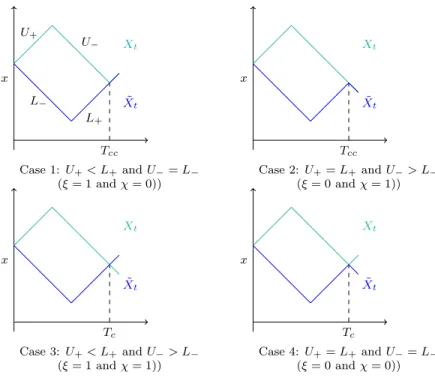
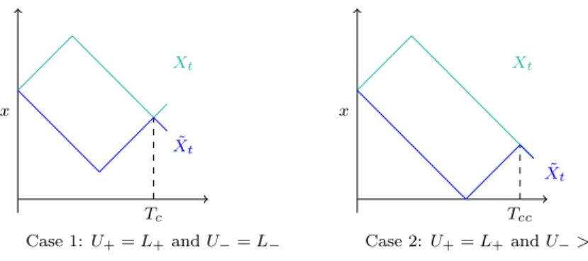
Let us denote by T_(x,v) the first jump time of the stochastic process (X, V ) starting from (X0, V0) = (x, v) with infinitesimal generator defined by (2.3). This random time satisfies

T_(x,v)= inf ⇢ t 0 : Z t 0 c(Xs)ds E ,

where E is an exponential variable with unit mean and c stands for the function b when v = +1 and, when v = 1,

c(x) = (

a(x) for x > 0, +₁ for x_{ 0.}

The process (X, V ) being deterministic between jump times, we have T(x,v)= inf ⇢ t 0 : Z t 0 c(x + vs)ds E .