Analysis Strategies for Marine Icing and Impact Module Images

(1)

Publisher’s version / Version de l'éditeur:

Vous avez des questions? Nous pouvons vous aider. Pour communiquer directement avec un auteur, consultez la Questions? Contact the NRC Publications Archive team at

PublicationsArchive-ArchivesPublications@nrc-cnrc.gc.ca. If you wish to email the authors directly, please see the first page of the publication for their contact information.

https://publications-cnrc.canada.ca/fra/droits

L’accès à ce site Web et l’utilisation de son contenu sont assujettis aux conditions présentées dans le site LISEZ CES CONDITIONS ATTENTIVEMENT AVANT D’UTILISER CE SITE WEB.

Student Report; no. SR-2009-04, 2009-01-01

READ THESE TERMS AND CONDITIONS CAREFULLY BEFORE USING THIS WEBSITE.

https://nrc-publications.canada.ca/eng/copyright

NRC Publications Archive Record / Notice des Archives des publications du CNRC : https://nrc-publications.canada.ca/eng/view/object/?id=959d851a-ffc7-4e9f-bc03-9114e1f8ad4a https://publications-cnrc.canada.ca/fra/voir/objet/?id=959d851a-ffc7-4e9f-bc03-9114e1f8ad4a

NRC Publications Archive

Archives des publications du CNRC

For the publisher’s version, please access the DOI link below./ Pour consulter la version de l’éditeur, utilisez le lien DOI ci-dessous.

https://doi.org/10.4224/18227305

Access and use of this website and the material on it are subject to the Terms and Conditions set forth at Analysis Strategies for Marine Icing and Impact Module Images

(2)

National Research Council Canada Institute for Ocean Technology Conseil national de recherches Canada Institut des technologies oc ´eaniques

SR-2009-04

Student Report

Analysis Strategies for Marine Icing and Impact Module

Images.

(3)

DOCUMENTATION PAGE REPORT NUMBER SR-2009-04 NRC REPORT NUMBER SR-2009-04 DATE April 24, 2009

REPORT SECURITY CLASSIFICATION

UNCLASSIFIED

DISTRIBUTION

UNLIMITED

TITLE

ANALYSIS STRATEGIES FOR MARINE ICING AND IMPACT MODULE IMAGES

AUTHOR(S)

Lian Feng Li

CORPORATE AUTHOR(S)/PERFORMING AGENCY(S) PUBLICATION

SPONSORING AGENCY(S)

IOT PROJECT NUMBER NRC FILE NUMBER KEY WORDS

Image Analysis, Marine Icing, Ice Impacts

PAGES 86 FIGS. 23 TABLES 1 SUMMARY

Image analysis strategies have been developed and shown to be useful for analyzing images from marine icing events to obtain quantitative time series icing thickness measurements. The same techniques were also found to be very effective for acquiring pressure data from images from a novel opto-mechanical pressure sensor technology that is incorporated in a new ice impact panel.

ADDRESS National Research Council

Institute for Ocean Technology Arctic Avenue, P. O. Box 12093 St. John's, NL A1B 3T5

(4)

National Research Council Conseil national de recherches Canada Canada

Institute for Ocean Institut des technologies Technology océaniques

ANALYSIS STRATEGIES

FOR MARINE ICING AND IMPACT MODULE IMAGES

SR-2009-04

Lian Feng Li

(5)

Table of Contents

1 INTRODUCTION--- 1

2 IMAGE ANALYSES FOR MARINE ICING EVENT --- 1

2.1 Marine Ice --- 1

2.2 MIMS --- 1

2.3 Previous Technique for Analyzing Marine Icing Images --- 4

2.4 Analysis Technique Improvement --- 6

3 IMAGE ANALYSES FOR IMPACT MODULE --- 9

3.1 Impact Module--- 9

3.2 Technique for Analyzing Impact Module Images---10

3.2.1 Image Processing---10 3.2.2 Edges Measurement ---12 3.2.3 Figure Image ---14 4 CONCLUSION ---16 REFERENCES---33 List of Appendices Appendix A: Python Code for Analyzing Marine Icing Images---34

Appendix B: Analysis Results for Maine Icing image ---43

Position 4 (A Vertical Pipe Structure) ---43

Position 12 (A Round Structure)---45

Position 17 (A Rail Structure)---47

Appendix C: Python Code for Analyzing Impact Module Images ---49

Appendix D: Analysis Results for Impact Module images---57

Test 1 ---57

(6)

List of Figures

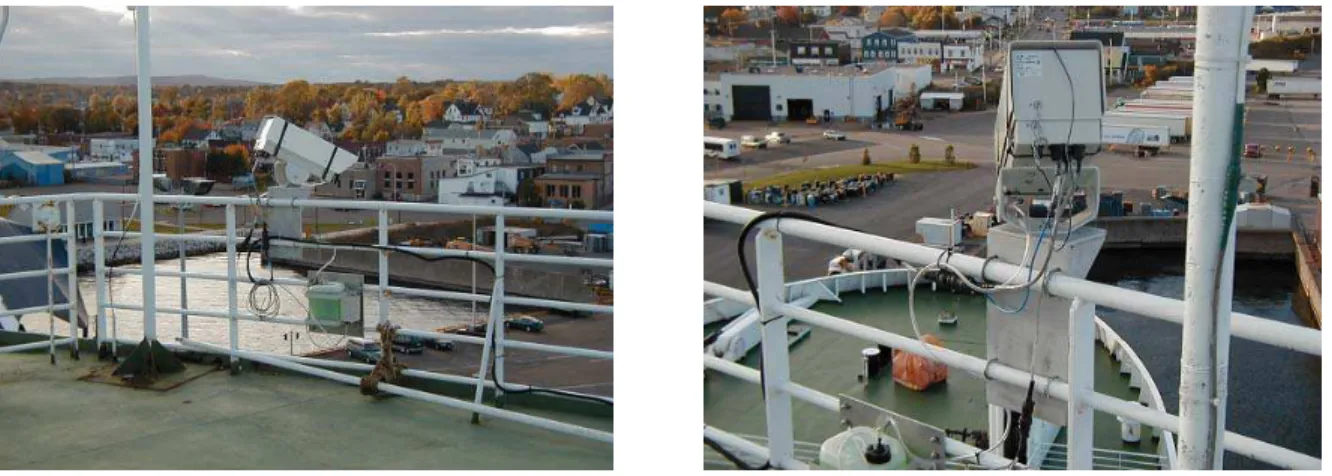
Figure 1: Cameras attached on upper deck rail --- 2

Figure 2a. Spray Image --- 3

Figure 2b. Water on Deck --- 3

Figure 2c. Snow on Deck --- 3

Figure 2d. Ice covered (Camera’s) Window --- 3

Figure 2e. Ice on Vessel--- 3

Figure 3. Selected positions for analysis--- 4

Figure 4. Image processing --- 5

Figure 5. Matplotlib plotting --- 5

Figure 6. The plots of average intensity array--- 7

Figure 7. Results for vertical structure --- 8

Figure 8. Results for eclipse structure--- 8

Figure 9. Sectional view of the Impact Module--- 9

Figure 10. Sectional view of the sensor ---10

Figure 11. White region on a strip ---10

Figure 12. Impact Module test ---10

Figure 13. Image before processing ---11

Figure 14. Processed by blacking components---11

Figure 15. Zoomed object after image processing---12

Figure 16. Not resized and resized image ---12

Figure 17. Image programmed by Python ---14

Figure 18. Measurements drew line on object and plotted as a figure image ---14

Figure 19. Figure image plotted for Figure 17 ---15

List of Tables Table 1. Summary of MIMS observations during winter of 2007/2008 deployment on the Atlantic Eagle---17

(7)

1 INTRODUCTION

Image analysis strategies have been developed and shown to be useful for analyzing images from marine icing events to obtain quantitative time series icing thickness measurements. The same techniques were also found to be very effective for acquiring pressure data from images from a novel opto-mechanical pressure sensor technology that is incorporated in a new ice impact panel. Marine ice accumulation on vessel causes many safe issues during navigation. Mr. Robert Gagnon, a research officer in Canada’s Institute for Ocean Technology (IOT) designs the Marine Icing Monitoring System (MIMS) to research the icing event on the vessel. Python is a simple computer programming language, which used to analyze the image from the system. The technique is automatic and can be applied in different strategies. The images from Impact Module provide the test information of dropping an ice block on the Module, and the analysis technique is able to analyze the images because the test information is recorded on the width of the object and can be calculated from the measurements.

2 IMAGE ANALYSES FOR MARINE ICING EVENT 2.1 Marine Ice

Ice accumulation on vessels is usually caused by fog, freezing rain and sea spray accumulating on the superstructure or hull, and freezing under their freezing points. The freezing point of seawater varies with the quantity of salt. The average quantity of salt in the sea is about 34.48%, so the freezing point of seawater is about –1.9 degrees Celsius. From analyzing the quality of the ice on vessels, we find that the sea spray has the most significant impact on vessel icing. Sea spray is when sea waves collide with the hull of a high-speed vessel, and spray up large amounts of seawater to the deck and superstructure. Most of the seawater flows back into the sea through the rail and the rest will evaporate in good weather condition. In contrast, the seawater will freeze in cold weather and the ice sublime slowly. Consequently, the total weight of the ship is increased by holding the solidified seawater. The solidified seawater, which is caused by sea spray under low temperature and certain wind speed, is defined as marine ice.

Marine ice exists as long as the temperature is lower than –1.9 degrees Celsius, and the amount of the ice will increase if the seawater continually sprays up to the deck under this condition. As the ship moves forward, the ice accumulating at the bow is more than the ice at the stern. If too much ice accumulates, the stability of a ship will be weakened. The longitudinal trim moment will be increased if the weight adding far away from the center of flotation is unbalanced. Increasing the distance between forward draft and afterward draft raises the angle of a ship rotating about its transverse line. A large angle of rotation will increase the chance of a ship to trim over, which will provide a low safety standard for sailors during navigation. In order to enhance the icing strength of a boat, researchers need to find the maximum icing impact and provide necessary emergency warning. The requirement of researching ice impact is to collect detailed data from ice accumulation.

2.2 MIMS

In order to collect the data of vessel icing, the Marine Icing Monitoring System (MIMS) is designed for monitoring the event on the boat. MIMS consists of two high-resolution cameras, a computer enclosure, a telephone enclosure and a power enclosure. All instruments are constantly supplied by a standard 110 VAC power in the power enclosure, and are connected by cables. The

(8)

environment. The cameras are set up separately on the Starboard and Port upper deck rail of a vessel, and they both face down to the bow (shown in Figure 1). In order to prevent the ice frozen on the windows from accumulating, researchers in IOT also equip heaters with both cameras. Two cameras are taking pictures every twelve minutes but the time is different, because the computer enclosure is programmed to offset the cameras’ operation by six minutes. For example, the starboard camera captures an image at seven o’clock. The port camera will capture an image six minutes later. When the computer enclosure receives images from cameras, it automatically minimizes the quantity of pictures to thumbnail images, and stores them with the originals to its hard drive. The computer enclosure is connected to a telephone enclosure, which can be a remote control for the operator in IOT. Because the thumbnail pictures have smaller size, and are faster to download, the operator always checks the operation of the system by viewing thumbnail images through a satellite phone in the telephone enclosure. Through the telephone enclosure, the system can be turned off at night and the period of system error by the operator in IOT as well.

Figure 1: Cameras attached on upper deck rail

IOT cooperates with Marine Atlantic and Petro Canada, so the MIMS is installed on their boat. The whole system is waterproof, and two cameras are strongly attached on the upper deck rail. After observing the performance of the system, the window of the camera is always covered by ice during snow, freezing rain or marine icing conditions. Dealing with this problem, the researcher in IOT develops a new heater, which is a heat transfer material in the middle of the window. The material is colorless and has high resistance. After the material is electrified, the window warms up, and the ice is hard to freeze on it. The new heater will be installed on the system in 2009.

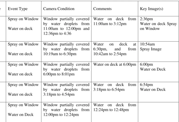
The MIMS was installed on the vessel of Atlantic Eagle from November 2007 to April 2008. The data of surveying six months’ images is documented as Table 1. All images are named as the time when they are taken, and every image indicates the event happening at this time. Table 1 records all potential events that happened in these six months, such as spray image (Figure 2a), water on deck (Figure2b) and snow on deck (Figure 2c). The table also notes the time period of ice covering the window of the camera (Figure 2d), which is a reference for researchers in IOT to check the ability of the heat in the camera. The most important event is ice on the vessel, which is shown in Figure 2e. The vessel is icing for a long period of time, and the images during this time are what we need to analyze.

(9)

Figure 2a. Spray Image Figure 2b. Water on Deck

Figure 2c. Snow on Deck Figure 2d. Ice covered (Camera’s) Window

(10)

2.3 Previous Technique for Analyzing Marine Icing Images

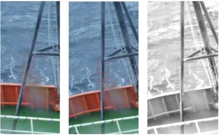
For surveying the rate of ice accumulation, the selected icing events should continue as long as possible. The Starboard images at daytime of Dec 29, 2006 provide more than forty continuous icing events. Two cameras are orientated to the bow; hence, all components in each image have the same location. The images show very a detailed marine icing process. The first few images have no icing event, and the marine ice is accumulating on the vessel along with time passing. We cannot only distinguish the increasing ice thickness, but also view many sea sprays during the time period. As a result, these images are treated as analysis research material for measuring ice thickness.

Leah Gibling first claims a manual method of measuring ice thickness in the report “Marine Icing Events: An Analysis of Images Collected from the Marine Icing Monitoring System (MIMS)”. She notes that the measurement is to count pixels between two edges of the selected position for each iced accumulated image, and then compares the record result with the image with no icing event. All measurements are recorded in a Microsoft Excel spreadsheet, and the software will display a linear graph to show the ice growth. The measurement is accurate but it takes too long to measure, so it is desirable that the analysis method be automated.

Based on Gibling’s method, Wayne Bruce programs an automatic image analysis method in Python in winter 2008. Python is an object-oriented programming (OOP) language, which provides a variety of modules. Comparing with C++, Python programming language is much easier to learn, and the code does not need to have a main function. Python is supported by many kinds of libraries, and the Python Image Library (PIL) is very useful to analyze ice event images. PIL is widely used in processing lattice images for Python. PIL lists the intensity of each pixel for interpreters to input an image to their code. The code contains the image for interpreters to analyze, and they can change the values of intensity, thereby changing the output of the image. Depending on the property of PIL and the method from Gibling, Bruce programs a Python code to count the pixels between edges of the selected structures that are shown in Figure 3.

(11)

The process of the code can be divided into three steps. The first step is image processing. The image is rotated for making the selected position to be linear and then color enhance and greyscale the image in order to convert the intensities to single values. Thereafter, the image is modified by the edge find command and cropped the selected position in PIL. The image is converted into black except the edges are shown in white, so that intensities between white edges and other black components are obviously distinguished. The procedures of processing image are shown in Figure 4. After the image is processed, the linear position is cropped by placing the object in the middle and prepared for the second step, which is edge measurement. The intensities of the cropped image are listed into a matrix, and the size of the matrix is along with the cropped image’s width and height. The edges have high intensity values, and to find the location of the maximum values in each row will give the width of the edge. The locations of the edges in the cropped image are drawn line, and the measurements are recorded for the last step to plot. In addition to plot a graph of measurement, Bruce imports a plotting library called Matplotlib. Matplotlib is able to produce a variety of two-dimensional figures for Python interpreters. Figure 5 shows a Matplotlib plotting of an icing event. The points stand for measurements, and time process axis is the number of images.

(12)

Relying on the computer’s high-speed calculation, image analysis by Python is much faster than analyzing manually. Although the image analysis method is approaching automatic, the measurements may be worse than when measured manually. As shown in Figure 5, there are more than forty input images, but only output twenty-one points in the graph, which means the code provides lots of bad measurements and deletes them automatically. Therefore, improving Bruce’s automated analysis method is necessary.

2.4 Analysis Technique Improvement

The plots received by Bruce have no certain scale and are missing many points because the code contains error filters. These filters delete some measured results and rearrange the result array without recording the position of the deleted point in the array. As a result, the graph is only a plot for results versus the number of filtered results, and has no relationship with the edge measurements. If the measured results are wrong, it is in vain to attempt to filter the measured results. In order to improve the image analysis, the code should be improved to measure edges properly.

Python software has no syntax inspection, and interpreters can only find syntax error if they run the whole program. It is known that Eclipse software is widely used for programming because it not only provides both syntax and logical inspections but also outputs the error and specifies the reason. Installing Python on Eclipse with import PIL, Numpy and Matplotlib libraries, the efficiency of improving automated analysis in Python is developed. The Numpy library is built by numeric structures which provide scientific computation for Python interpreters.

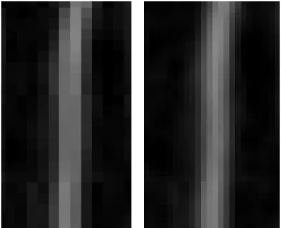
The automatic analysis method is to count the number of pixels between the two brightest points in a cropped image. In spite of a large amount of brightest points contained in the object’s edges after the edge find is processed in Python, messy backgrounds also provide some brightest points, which influence the measurement. For the purpose of cleaning these bad brightest points, the positions selected from the original image should avoid a background with complex structure. A background with complex structure can be avoided by cropping clean background images, and the sizes of the cropped images are varied. We process the image by using the PIL, and crop the position that we want to analyze.

We convert the cropped image into an intensity matrix and researched the method of edge measurement. We design three methods to analyze the intensity matrix, and the standard method is to average the intensities at each column of the matrix. The edge-detected image has its color converted into black, except the edges are shown in white. The intensity for white is 255 and for black is 0. After we average the of intensities at each column, the intensity matrix changes to be an array, and the values standing for edges should be greater than other values in this array. This method is able to analyze a cropped image with a messy background, because the value calculated by averaging the intensities in one column nears the intensities that have a large amount in this column. Most of the intensities in the background are approaching to zero; therefore, if few amounts of the bright points are in the cropped image’s background, the intensities of the bright points will be changed to approach zero after the average of each column of the intensity matrix.

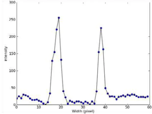
Figure 6 plots the average intensity array created from the edge-detected image, which is shown in Figure 4. The values in the graph standing for the black background with some white points do not vary too much, and the two peak values which stand for the brightest points should be inside of the white edges, so we will find the edges’ location in the array if we find the location of the two peak values. As shown in Figure 6, the peak values located inside of the edges, and the locations of the actual edges, normally distribute at a few points before the peak values. As a result,

(13)

percentages are varied based on the positions at input image. For example, we set the actual edges’ intensities at 65% of the peak values for both edges in a pipe structure, and set the left edge of a rail structure at 25% and the right edge at 80% of the peak values. After the first brightest points in both hands are found, the location of these intensities in the array will be recorded for drawing lines standing for edges on the object in cropped images. The cropped images are combined together and separated by white lines. Each combined image includes only one selected position in all analysis images, so each point in the plotting graph can be expressed as a cropped image. The plot contains a polynomial line which indicates that the ice thickness has no certain increasing rate.

Figure 6. The plots of average intensity array

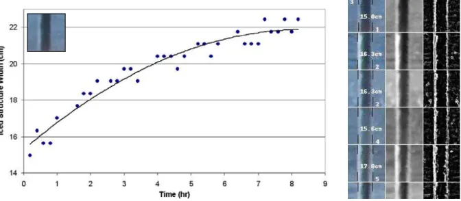
This method not only analyzes the vertical object, but also works well for analyzing a round structure. We rotate the round structure and cut one piece from the area that locate at the horizontal centerline of the structure, so the analysis method is used to analyze two curved lines. The object has a shape of parenthesis, and the intensities are symmetrical distributed from the object’s horizontal centerline. When we sum the intensities at each column of the cropped piece, the intensities that locate at the centerline will be half of other intensities. In other word, when we measure the points of the maximum width in two curves, the intensities of two top points of the curved lines should be half of the peak values after averaging each column of the intensity matrix. Two curves are symmetrical from the maximum width, so the two end points of the maximum width are half of the other points on the curves after averaging the intensities at each column of the image. After the maximum width is found, the code draws lines on the centerline from both sides of the cropped piece to the maximum width of the object. Compared with applying the method to analyze the whole round structure, analyzing the cropped piece can avoid the messy background and unclear edges in the structure. Because of the terrible weather conditions during navigation, the captured image may have some fuzzy structures. The more fuzzy edges we analyze, the more uncertainty we get for the measurements. Figure 7 shows the measured results for a vertical structure, position 3, and Figure 8 shows the results for an eclipse structure, position12.

(14)

Figure 7. Results for vertical structure

Figure 8. Results for eclipse structure

An alternative method of analysis of the intensity matrix would be to analyze the intensities at each row of it. This method is to change the matrix into many arrays. The length of them is the same as the width of the matrix, and the number of them is the same as the height of the matrix. We assign the code to analyze each array from both sides to the middle of it, and the two first bright points at each array will be recorded as the edge location. After we finish analyzing the matrix, we average the measurements and the two results will be the edge locations. Another alternative method of analysis of the intensity matrix is to increase the quantity of the image, which is to resize the image. We cannot measure the edge increasing in one pixel because the resolution of the camera limits the quantity of the image. As a result, we resize the image to double the number of pixels along the x- and y-axes. The number of pixels inside of the edge is double, so the edge increasing in one pixel can be measured. The alternative methods have a good performance

(15)

standard method. On the other hand, the alternative methods can be performed easily to measure the ice thickness in a clean background image. However, we apply these methods to analyze the images from Impact Module.

3 IMAGE ANALYSES FOR IMPACT MODULE 3.1 Impact Module

When a ship navigates in arctic conditions, the amount of ice is enough to trip the ship or even sink it. The so-called “unsinkable” ship, Titanic, was sunk by icebergs in 1912. In 2007, the Explorer was turned over by impact with a chunk of ice. Even though nowadays ships are designed with high technology to be stronger than before, marine disasters caused by ice impact are still happening. In order to research the nature of forces and their distribution during a collision, Robert Gagnon in IOT designed an impact module to test the ice impact.

The Impact Module is constituted by a sensor, a large acrylic block and a high-resolution camera, and the sectional view of it is shown in Figure 9. The sensor is applied with pressure technology and it is able to measure accurately the pressure distribution. The sensor is shown in Figure 10 and it is composed of many pressure strips. Each strip has a very slight curvature. They are arranged on the top of an acrylic block and face down with their curved surface to the block. When one strip is pressed, the curved surface will contact the acrylic and create a white region. The white region of one strip is shown in Figure 11. The width of the white area is proportional to the applied pressure. The sensor is covered by a thin metal sheet which will protect strips during an impact. The sensor is put on the top of the acrylic block. The acrylic block is transparent and with the dimension by one meter of one meter square and half a meter in thickness. Two lights are installed in the thick acrylic block so that the white region created by strips will be obvious. The acrylic block is very strong; therefore, the camera behind it is protected during collisions. When ice impacts the module, the pressure and its contact area are changed rapidly. As a result, the installed camera has high resolution and it is able to capture 250 images in one second.

(16)

Figure 10. Sectional view of the sensor Figure 11. White region on a strip To test the Impact Module, a large block of ice is raised by crane and the center of it is directly over the middle of the sensor. As the ice is released, images taken from the camera are delivered to a computer to analyze. Figure 12 shows the steps of the experiment. In the future, the impact module will be created as a large version and installed on an icebreaker to collect actual data. The collected data will be provided for designing ships to operate safely in arctic conditions.

Figure 12. Impact Module test 3.2 Technique for Analyzing Impact Module Images

The image analysis method of the Impact Module is similar to the analysis of the Marine Icing Event. Python programming is used to analyze images with import PIL, Numpy and Matplotlib libraries. Based on the property of color intensity, the code automatically counts the pixels between edges from analyzing an image that has converted to an intensity matrix. Compared with the method of analysis Marine Icing images, the analysis technique for the Impact Module has been improved. The input image has already been processed by Paint Shop Pro, and the analysis method is applied to the whole image.

3.2.1 Image Processing

The fabrication of the Impact Module is not perfect. The acrylic block contains many bubbles and some equipment components inside of camera view, shown in Figure 13. The measurement

(17)

edges in the input image. To ignore the effect of these components, we black the components area by programming so that the measurement will not work on them. Figure 14 shows an image after the process of black components. Furthermore, the bubbles that affect the test exist in the big acrylic block because of the uncertainty during producing the acrylic block. After we analyze an image with large amounts of bubbles, the edge measurement will be nonsense, so it is necessary to clean the bubbles in future experiments.

Figure 13. Image before processing Figure 14. Processed by blacking components In addition to clean the bubbles in an image, we introduce the software of Paint Shop Pro. Paint Shop Pro contains many professional image processing toolbars that assist us to create good images by modifying their weakness. For example, after edge detected is processed by Python programming, thin edges in an image will be unclear because the process image is automatically sharpened. However, the edge effect toolbar in Paint Shop Pro contains horizontal and vertical edge detection so that the found edges are much clearer than those processed by Python. In order to clean bubbles in an image, Mr. Gagnon uses the subtract toolbar in Paint Shop Pro to process objective images. He processes an image without containing the white region, and then creates a package of objective images to subtract the processed original image. The original image is processed by moving two pixels in each direction because along with the camera zooming an object, the bubbles move their position for one or two positions. As a result, Mr. Gagnon uses the toolbar to find the union of the four images, which are created by moving the original image upward, downward, left and right. The bubbles in the original are spread for two pixels. After the images are processed by subtract, the bubbles will be cleaned if they do not move or they move up to two pixels. The second step for processing the image is edge detection in Paint Shop Pro. Figure 15 shows the zoomed objects after image processing.

(18)

Figure 15. Zoomed object after image processing

For the purpose of researching the relation between actual width and the edge-detected width, Mr. Gagnon measures the number of pixels between edges, and he found that the actual width always is the distance between two brightest points in the edge detected image. The edge-detected image is very clean and has no complex structure, so we decided to increase the quantity of the processed image which is to resize the image. Figure 16 shows the observation of the not resized and the resized image. After resizing the image, the number of pixels is double along the x- and y-axes, and especially the number of pixels inside of the edge is double. The code selects the brightest point as an edge. As we can see from Figure 16, the not resized image has two bright points in an edge so the code will choose a brighter one as an edge. The resized image has five bright points in an edge so the code will select an edge from five points. The uncertainty of measuring width is decreased at least fifty percent by resizing the image.

Figure 16. Not resized and resized image 3.2.2 Edges Measurement

(19)

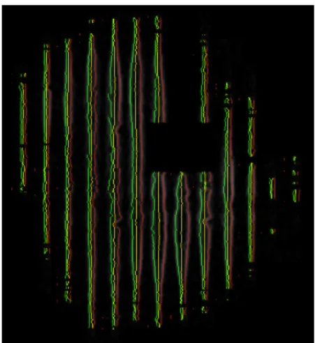
directed to the middle of the sensor in the experiment, the contact area may not only appear in the middle because the air resistance may change the direction of the block before collision happens. Therefore, we have to analyze the whole image without cropping a certain position by using Python programming with import PIL. On the other hand, we know that the width of each pressure strip is the same, so the whole image can be separated into many slices, and each of them has the same width as a strip. The code is assigned to analyze each slice, and it only provides results from measuring the width of the white region. The white region only appears under each pressure strip, so we need to make sure that each slice is the area of the strip. Besides, the white region has no certain shape. It may be a thin rectangular or a white area with many random shapes. In order to measure the width of an object with no certain shape, we decide to use the method of analyzing each row of the intensity matrix. We convert the slice into an intensity matrix and assign the code to find two peak intensities in each row. We also assign the code to measure edges only if the highest intensity is greater than zero so that the code will not analyze the black area in the image. We divide the image into many slices and analyze each of them. We use the method to find the edges locations at each row of the matrix, but we do not average the measurements of the matrix because the object has uncertain shape and each measurement is the information that we want to analyze. In spite of the white regions’ random distribution in the image, Python programming can be used to measure their width because the intensity of the black background is distinguished from the white edges.

In addition, the middle of the white region cannot be defined as the same as the middle of the slice. For instance, some parts of the white region may appear at the left side of the slice. The method to find the edge from both sides to the middle of the slice failed because the middle of the object varies. With regard to find the middle of the white region in the image, we introduce a new idea which is color intensity moment. The color intensity moment can be used to define the middle line of the white region. To analyze one row of the matrix, we assign the code to add the multiplication of intensities and their locations in the row, and then divide the sum of all intensities in this row. The position of the resulting intensity is measured in this row. After we analyze each row of the slice, a nonlinear middle line is created. Compared with the black background, two edges have relative high intensities so that the position of the resulting intensity should be located in the middle of them. After that, we command the code to find the brightest point from both sides of the slice to the middle line that is created by the color intensity moment.

The measurement is accurate even if the object is located in one side of the image. After the code finishes measuring the edges, it automatically draws lines standing for edges and middle line. Figure 17 is a zoomed image that is programmed by Python. The green lines and red lines stand for left and right edges, and the yellow lines are the middle line that is defined by the color intensity moment. Each slice of the image is drawn lines and combined together by PIL. We also number each slice by the number on the top of each analyzed slice, so we can check the operation of the test by checking the lines drawn on proper edges. If there are lines drawn on wrong edges, we will fix the input image by blacking the messy points. The messy points are created by cleaning bubbles in the image process. Some white regions contain bubbles before image processing, and these bubbles will leave their curves on the white region after image process. The curves may increase or decrease the width in some parts of the white region, and create some bad points in the processed image as well.

(20)

Figure 17. Image programmed by Python 3.2.3 Figure Image

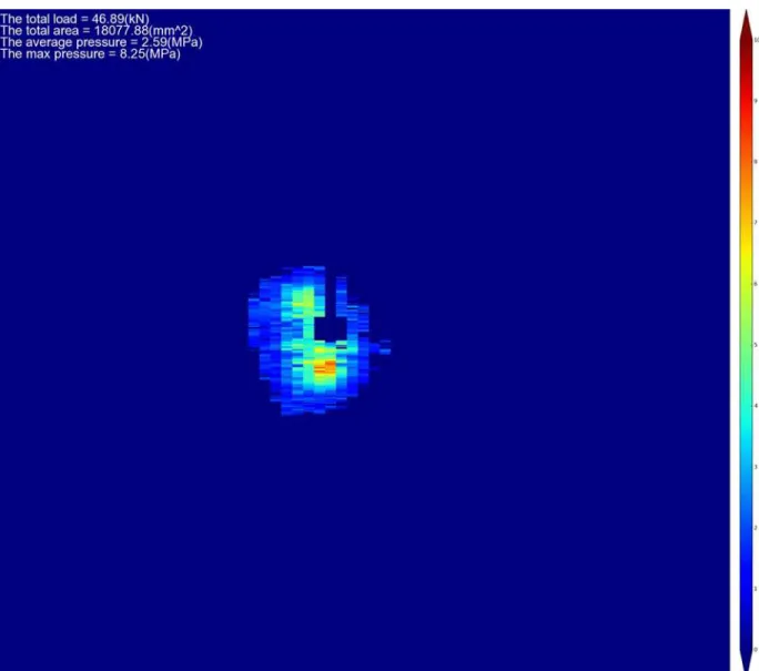
Python programming not only draws lines standing for measurements on the object, but also makes a figure image for shown test results. The figure image provides a color bar for showing the contact area and pressure distribution, and also recodes the maximum pressure, average pressure, total load and total contact area. The figure image is a color plot for analyzing the input image. The code plots small figure images for each slice, and then combines them together. We use the Matplotlib library to plot a value into a pixel with a certain color. For example, the code saves all measurements into a one-dimensional array after analyzing one slice. If we plot a figure image for this array, the figure image will have the same height as the slice but the width of the image is only one pixel. As a result, we need to reduplicate each value in the array. We assign the code to reduplicate the value to have the same amount of pixels in the width of the slice. Based on the range of the pressure that we measured, we create a color bar to show the pressure distribution in the figure image. The range of the color bar is defined from zero to ten, and the chroma is changed from blue to red. The white regions caused by applied pressure are drawn lines on their edges, and the measurements are plotted as a figure image, which is shown in Figure 18.

(21)

PIL cannot be used to combine the figure image created by the Matplotlib library because the figure image created by Matplotlib cannot input to the PIL. The PIL only recognizes the image file with the extension such as “png” and “jpeg”. Therefore, we create a temporary file with the extension of “png” to save a figure image created by Matplotlib, and then assign the code to load the file into the PIL. After the second figure image is created, it will be saved into the same temporary file so that the previous image in the file will be replaced, and then we load the second image into PIL again. By this method, we can load all figure images, which contain all slices of the input image and a color bar, into the PIL to combine together. After that, we also draw text on the combined image to record the maximum pressure, average pressure, total load and total contact area, and these values are calculated based on the width of the white region. Figure 19 shows the figure image plotted for Figure 17. At the end of analyzing the input image, we use the close command to close all temporary data. The temporary data is created during the procedure of analysis. If too much temporary data is created, the speed of analysis will be decreased and the whole system will be slow or even crash.

(22)

4 CONCLUSION

Seawater spraying up to its superstructure under the temperature lower than -1.9 degrees Celsius and with certain wind speed leads to Ice accumulation on a vessel. Large amounts of ice accumulation on a vessel will weaken a ship’s stability which is threatened to sailors’ safety. To develop MIMS on monitoring marine icing event is able to assist researchers in IOT in measuring the growth of the ice thickness, and provide information to enhance the icing strength of a vessel. Based on the property of color intensity, Python programming is used to analyze the marine icing images. The code automatically plots the results and draw lines on the edges of the object. The technique has a good performance on both vertical and round structures. Thus, we apply the technique to analyze the object with no certain shapes. The objects inside of the images from Impact Module have random distribution and no certain shape. We improve the technique to operate well on measuring the Impact Module images, and the analyzed data will provide for designing a ship to operate safely in arctic conditions. Therefore, to improve the image analyzing technique will increase the ability to measure the width of an object, and the measurement could be a good reference to assist researcher in surveying the property of the object.

(23)

Table 1. Summary of MIMS observations during winter of 2007/2008 deployment on the Atlantic Eagle

Date

Start Time (on file) GMT + 1hr

End Time Event Type Camera Condition Comments Key Image(s) 11/28/2008

Starboard Camera

11:00am 4:36pm Spray on Window Water on deck

Window partially covered by water droplets from 11:00am to 12:00pm and 12:36pm to 4:36

Water on deck from 11:00am to 3:12pm

2:36pm

Water on deck Spray on Window

11/28/2008 Port Camera

10:19am 6:30pm Spray on Window Water on deck

Window partially covered by water droplets from 10:19am to 6:30pm Water on deck at 6:30pm, and from 10:42am to 2:54pm 10:54am Spray Image 11/30/2008 Starboard Camera 6:00pm 8:01pm Spray on Window Water on deck

Window partially covered by water droplets from 6:00pm to 8:01pm Water on deck at 6:00pm 6:00pm Water on Deck 11/30/2008 Port Camera 3:18pm 6:54pm Spray on Window Water on deck

Window partially covered by water droplets from 3:18pm to 4:54pm

Water on deck from 3:18pm to 6:54pm 6:54pm Water on Deck 12/01/2008 Starboard Camera 12:00pm 12:48pm Spray on Window Water on Deck

Water on deck from 12:24pm to 12:48pm

(24)

12:06pm 1:06pm Water on Deck Clear Water on deck from 12:06pm to 1:06pm

12/02/2008

Starboard/Port Camera

5:25am 9:01pm Spray on Window Window partially covered by water droplets from 5:25am to 9:01am, 10:13am to 10:48am and 8:25pm to 9:01pm (may caused by rain) 12/03/2008 Starboard Camera 2:24pm 6:00pm Spray on Window Water on Deck

Window partially covered by water droplets from 2:24pm to 2:48pm Water on deck at 3:24pm and from 12:24pm to 1:00pm, 4:00pm to 4:36pm 6:00pm Wave/Spray Image 2:36pm Spray Image 12/03/2008 Port Camera

12:42pm 2:18pm Water on Deck Clear Water on deck from 2:06pm to 2:18pm 12:42pm Wave/Spray Image 12/04/2008 Starboard Camera 12:12pm 5:36pm Spray/Ice on Window Water on Deck

Window partially covered by water droplets from 1:00pm to 1:24pm and 4:00pm to 5:36. Camera fully covered by ice from 2:36pm to 2:48pm, and partially covered from 1:36pm to 1:48pm

Water on deck from 12:12pm to 2:24pm and 3:00pm to 3:24pm

Ice on window may be caused by frozen rain

2:36pm

Ice on Window 3:12

(25)

2:30pm 4:18pm Spray and Ice on Window

Ice on Deck

Window partially covered by water droplets from 2:30pm to 2:54pm, 3:54pm to 4:18, 4:59pm to 5:30pm. Camera fully covered with ice at 1:54pm and 2:42pm (may caused by frozen rain)

Ice on deck from 2:54pm to 3:54pm (may caused by frozen rain) 12/07/2008 Starboard Camera 12:12pm 4:36pm Spray on Window Water on Deck

Window partially covered by water droplets at 12:12pm, 1:12pm and 4:36pm

4:00pm Water on Deck

4:42pm 5:42pm Spray on Window Window partially covered by water droplets from 4:42pm to 4:54pm 4:54pm Wave/Spray Image 12/10/2008 Starboard Camera

8:01am 7:24pm Ice on Window Ice and Water on Deck

Window partially covered by ice from 8:01am to 8:37am and 10:12am to 12:36pm

Ice on deck melted at 7:24pm

1:00pm

Water and Ice on Deck

(26)

10:19am 7:55pm Spray and Ice on Window

Ice and water on Deck

Window partially covered by ice from 10:19am to

10:42am. Window partially covered by water

droplets from 11:42am to 12:06pm (may caused by rain)

Water on deck from 7:30pm to 7:55pm 12/12/2008 Starboard Camera 6:00pm 7:00pm Ice/Spray on Window Ice on Deck

Window partially covered by water at 6:00pm, and from 7:12pm to 7:49pm. Window fully covered by ice at 6:12pm, and partially covered from 6:24pm to 7:00pm

6:12pm Ice on Window

5:42pm Snow and Ice on Deck

Spray and Ice on Window

Window partially covered by ice from 6:06pm to 6:30pm, and covered by water droplets since 6:42pm (may caused by frozen rain)

Snow on deck from 5:42pm to 8:07pm

Ice on deck from 11:20pm to 11:43pm (may caused by snow or rain)

(27)

12/13/2008 Starboard Camera

10:37am 12/14/2008 12:38

Ice on Window Window fully covered by ice from 10:37am to 12:48pm, and partially covered after 1:00pm

Ice melted after 12/14/2008 12:38

11:24am Ice on Window

2:31am 3:06pm Ice/Snow on Deck Spray on Window

Window partially covered by water droplets from 3:19am to 3:31am (may caused by frozen rain)

Ice on deck from 2:31am to 3:31am

Snow on deck since 10:31am

Water on deck, pushing snow from 1:30pm to 2:06pm.

1:30pm Spray Image

Water on Deck Snow on Deck 12/19/2008 Starboard Camera 4:36pm 10:37pm Ice on Deck Ice on Window

Window partially covered by ice from 10:25pm to 10:37pm 10:25pm Ice on Window 12/20/2008 Starboard Camera

11:00am 4:00pm Ice on Deck Ice on Vessel

Clear Crews clear some ice at 4:00pm 1:48pm Spray Image Ice on vessel 12/20/2008 Port Camera

Clear Crews clear some ice from 3:54pm to 4:06pm 11:42am Spray Image Ice on Vessel 12/22/2008 Starboard/Port Camera

11:00am 7:48pm Ice on Vessel Clear Ice created on 12/20/2008

(28)

12/23/2008 Starboard/Port Camera

11:00am 7:37pm Ice on Vessel Clear Ice created on 12/20/2008

12/25/2008

Starboard Camera

1:12pm 3:24pm Water on Deck Clear Water on deck at 1:12pm, 1:48pm and 3:24pm

11:42am 7:30pm Water on Deck Clear Water on deck at 11:42am, 2:54pm and 7:30

7:30pm

Spray Image Water on Deck

7:12am 6:48pm Ice on Window Spray on Window

Window partially covered by ice at 7:12am, 9:12am and 9:36am. Window partially covered by water droplets from 10:36am to 4:00pm and 5:12pm to 6:48pm 9:36am Ice on Window 5:36pm Spray Image 12/28/2008 Port Camera

6:55am 9:31am Ice on Window Window partially covered by ice from 6:55am to 7:07am and 9:07am to 9:31am

6:55am Ice on Window

(29)

1:25am 1:00pm Spray and Ice on Window

Window partially covered by water droplets from 1:25am to 3:13am and 8:13am to 9:25am. Window partially covered by ice at 3:25am, and from 6:19am to 6:49am

Water on deck from 11:12am to 1:00pm 11:36am Water on Deck 12/29/2008 Port Camera 12:06pm 12:42pm Spray on Window Water on Deck

Water on deck from 12:06m to 12:30pm 12:06pm Water on Deck 12/30/2008 Starboard Camera 11:01am 7:24pm Spray/Ice on Window

Ice and Snow on Deck

Water on Deck

Window partially covered by water droplets from 11:01am to 11:14am and 1:00pm to 2:24pm. Window partially covered by ice from 11:24am to 12:00am, and fully covered at 11:36am

Wet snow on deck from 11:01am to 12:24am Ice on the deck from 11:01am to 1:24pm Water on deck at 3:00pm and 3:24pm,and from 5:48pm to 7:24pm

12:12pm

Snow and Ice on Deck

6:36pm

(30)

10:31am 8:07pm Ice and Spray on Window

Water on Deck

Window fully covered by ice at 10:31am, and from 11:18am to 12:18pm, and partially covered from 10:54am to 11:06am. Window partially covered by water droplets from 2:30pm to 8:07pm Water on deck at 2:30pm, and from 3:42pm to 8:07pm 11:30am Ice on Window 7:06pm

Water on Deck Spray on Window

10:00am 12:12pm Spray on Window Water on Deck

Window partially covered by water droplets from 10:00am to 12:00pm

Water on deck from 11:24am to 12:12pm

10:37am 1:48pm Snow and Water on deck

Window partially covered by water droplets from 11:01am to 12:12pm which may caused by rain

Wet snow on deck from 10:37am to 1:00pm

4:43am 4:54pm Snow and Water on deck

Spray on Window

Window partially covered by water droplets from 5:19am to 6:55am, 8:31am to 10:07am, 10:54am to 12:18pm which may caused by snow

Snow on deck from 4:43am to 12:06pm

12:30 pm

Water and Ice on Deck

(31)

11:18am 11:36am Water on Deck Clear Water on deck from 11:24am to 11:36am

01/17/2008

Port Camera

11:06am 6:42pm Water on Deck Spray on Window

Window partially covered by spray at 12:54pm Water on deck at 11:06am, 12:06, 1:42pm, and from 12:54pm to 1:06pm and 2:42pm to 6:42pm 12:54pm Water on Deck 01/21/2008 Starboard/Port Camera

10:00am 11:00am Ice on Window Window fully covered by ice from 10:49am to 11:00am 10:49am Ice on Window (Starboard) 01/22/2008 Starboard Camera

10:37am 8:24pm Snow on Deck Ice on Vessel

Ice/Spray on Window

Window partially covered by ice at 12:36am, 12:12pm, and from 4:00pm to 4:12pm. Window partially covered by water droplets from 5:57pm to 8:24pm

Wet snow on deck from 10:37am to 4:36pm Ice on deck melted at 7:24pm

Water on deck from 7:36pm to 8:12pm 12:12pm Ice on Window Ice on Deck 8:00pm Ice on Vessel 01/22/2008 Port Camera

10:19am 8:18pm Snow on Deck Ice on Vessel

Window partially covered by ice from 12:06pm to 12:30pm.

Wet snow on deck since 10:19am

7:54pm Ice on Vessel

(32)

Ice/Spray on Window

Clear Ice fully melted at 5:48pm

11:00am Ice on Vessel 01/23/2008

Port Camera

Clear Ice fully melted at 5:54pm 10:42am Ice on Vessel 4:18pm Spray Image 01/25/2008 Starboard Camera

10:49am 7:12pm Ice and Spray on Window

Ice/Water on Deck

Window fully covered by ice from 10:49am to 4:24pm (some images are all white)

Ice on deck from 4:36pm to 6:36pm

Water on deck from 6:00pm to 7:12pm 3:24pm Ice on Window 5:24pm Ice on Deck 01/25/2008 Port Camera

10:31am 6:18pm Ice on Window Snow on Deck and Vessel

Window covered by ice from 10:31am to 1:54pm (some images are white)

Snow and ice melted at 6:18pm 1:16pm Ice on Window 01/26/2008 Starboard Camera

4:00am Ice on Window Window fully covered by ice from 4:00am to 9:25pm (some images are black color), and from 01/27/2008 10:24am to 01/27/2008 8:00pm

(33)

10:43am 6:19pm Ice on Window Window covered by ice from 10:43am to 6:19pm Ship in port 6:19 Ice on Window Ship in Port 01/27/2008 Port Camera

2:30am 8:55pm Ice on Deck Ice on Vessel Clear 2:30am Ice on Vessel 3:18pm Ice on Vessel 01/28/2008 Starboard Camera

10:48am 9:00pm Ice on Window Ice on Vessel

Window partially covered by ice from 10:48am to 9:00pm 11:24am Ice on Vessel Ice on Window 01/28/2008 Port Camera

10:43am 8:56pm Ice on Vessel Clear Ship in port from 12:54pm to 1:38pm

Ice may be created before 12:06pm Ice on Vessel 02/03/2008 Starboard Camera

11:00am 5:48pm Water on Deck Spray on Window

Window partially covered by spray from 4:00pm to 5:12pm

Water on deck from 11:00am to 5:48pm 5:12pm Spray Image 02/03/2008 Port Camera 1:54pm 8:18pm Spray on Window Water on Deck

Water on deck at 8:06pm 2:06pm Spray Image 8:06pm Water on Deck

(34)

10:13am 4:24pm Ice on Window Window partially covered by ice from 10:13am to 10:48am Water on deck at 11:36am, 2:24pm, and from 12:00pm to 12:24pm, 3:36pm to 4:24pm 10:26am Ice on Window 2:24pm Water on Deck 02/05/2008 Port Camera

10:07am 3:54pm Ice on Window Window fully covered by ice from 10:07am to 10:54am Water on deck at 2:18pm, 2:42pm, and from 3:18pm to 3:54pm 10:54am Ice on Window 2:18pm Water on Deck 02/10/2008 Starboard Camera

2:24pm 9:01pm Water on Deck Window partially covered by water droplets from 2:24pm to 9:01pm

Water on deck at 2:24pm and 2:48pm, and from 6:36pm to 7:00pm

10:42am 4:06pm Water on Deck Clear Water on deck at 10:42am, 10:54am, and from 1:30pm to 4:06pm 10:42am Water on Deck 02/11/2008 Starboard/Port Camera

5:36pm 9:36pm Snow on Deck Clear Snowfall started at 5:36pm

(35)

5:15am 7:24am Ice on Window Starboard camera window partially covered by ice from 5:15am to 5:38am, 6:48am 7:24am. Port camera window partially covered by ice from 6:54am to 7:30am

Ice on Window may be caused by iced rain Ship in port

2:12pm

Water on Deck 02/19/2008

Port Camera

1:06pm 7:06pm Water on Deck Clear Water on deck at 1:06pm, 2:42pm and 7:06pm 2:30pm Spray Image Water on Deck 02/22/2008 Starboard Camera

10:00am Ice on Window Window fully covered by ice since 10:00am

8:00pm Ice on Window 02/22/2008 Port Camera 5:31am 02/23/2008 12:42am Ice/Snow on Window Snow on Deck

Window partially covered by ice/snow from 5:31am to 5:18pm, and fully covered since 5:30pm

Ice in window melted before 02/23/2008 12:42am 5:30pm Ice on Window 02/23/2008 Starboard Camera

10:24am 8:24pm Ice on Window Snow on Deck

Window fully covered by ice from 5:12pm to 8:24pm, and partially covered from 3:48pm to 4:12pm

Ice on deck caused by snow

7:48pm

(36)

3:30pm 11:42pm Ice/Snow on deck Ice on window

Window partially covered by ice from 3:30pm to 4:18pm, and fully covered by ice from 5:18pm to 8:18pm

Ice on deck melted before 11:42pm 7:06pm Ice on Window 02/28/2008 Starboard Camera 12:24pm 5:00pm Spray on Window Water on Deck

1:48pm

Water on Deck Spray on Window

10:18am 9:32pm Snow on Deck Clear Snow on deck since 10:18 (Some white images during this time), and melted before 03/01/2008 6:06pm 03/10/2008 Starboard Camera 12:00pm 5:48pm Snow on Deck Ice on Window

Window partially covered by ice from 12:24pm to 1:24pm

1:00pm Ice on Window Snow

on Deck 03/10/2008

Port Camera

11:54am 6:42pm Snow on Deck Ice on Window

Snow on deck melted before 6:42pm

Ship in port at 6:06pm

12:42pm

Snow on Deck and Window

(37)

4:06pm 5:18pm Water on Deck Clear Water on deck from 4:06pm to 5:18pm 4:18pm Water on Deck 03/26/2008 Starboard Camera

12:24pm 8:36pm Snow on Deck Clear 12:24pm

Snow on Deck 03/26/2008

Port Camera

8:55am 9:55pm Snow on Deck Clear Snowfall started at 03/25/2008 4:54pm 9:42am Snow on Deck 03/27/2008 Starboard Camera

5:36pm 6:36pm Ice on Window Window partially covered by ice from 5:36pm to 6:36pm.

Ice may be caused by frozen rain

5:48pm

Ice on Window 03/27/2008

Port Camera

12:55am 7:06pm Ice on Deck Ice on Window

Crews clear some ice at 11:54am

Ice may be caused by frozen rain 5:42pm Ice on Window 11:30am Ice on Deck 03/29/2008 Starboard Camera

11:00am 6:00pm Ice on Window Window covered by ice from 11:00am to 6:00pm

3:19am 12:42pm Snow on Deck Ice on Window

Window partially covered by ice from 3:19am to 12:42pm Snowfall started at 3:19am 9:30am Ice on Window 03/30/2008 Starboard Camera

12:36pm Ice on Window Window covered by ice since 12:36pm

Ice may be caused by frozen rain

4:00pm

(38)

12:42pm 5:54pm Ice on Window Window covered by ice from 12:42pm to 5:54pm

Ship in port at 4:18pm Ice may be caused by frozen rain 4:18pm Ice on Window 04/06/2008 Starboard Camera

9:12am Problem with Starboard Camera

Fuzzy Images There are many black or white images during this time 04/19/2008 8:36pm Fuzzy Image 04/14/2008 Port Camera

4:23pm 6:06pm Water on Deck Clear Water on deck from 4:23pm to 6:06pm 4:30pm Spray Image Water on Deck 04/15/2008 Port Camera

11:42am 12:18pm Water on Deck Clear Water on deck from 11:42am to 12:18pm

11:42am Water on Deck

(39)

REFERENCES

[1] Guido van Rossum, “Python Tutorial", <http://docs.python.org/tut/tut.html>, February 21, 2008.

[2] Python Imaging Library, “Handbook reference”,

<http://www.pythonware.com/library/pil/handbook/index.htm>, May 6, 2005.

[3] Darren Dale, Michael Droettboom, Eric Firing, John Hunter, “Matplotlib. Release 0.98.5.1” < http://matplotlib.sourceforge.net/Matplotlib.pdf >, December 17, 2008

[3] Leah Gibling, “Marine Icing Events: an Analysis of Images Collected from the Marine Icing Monitoring system (MIMS)”, Institute for Ocean Technology, 2007. SR-2007-07

[4] Wayne Bruce, “Automated Image Analysis For Marine Icing Events”, Institute for Ocean Technology, 2008. SR-2008-04

[5] R. Gagnon, M. Sullivan, W. Pearson, W. Bruce, D. Cluett, L. Gibling and L.F. Li, “Development of a Marine Icing Monitoring System”, Institute for Ocean Technology, 2009.

(40)

Appendix A: Python Code for Analyzing Marine Icing Images

import Image #PIL Python Image Library import ImageOps import ImageFilter import ImageDraw import ImageFont import glob, os import csv import time

from pylab import * frame = 100000

startTime = time.time() #record start time

calib = (0.68, 0.68, 0.68, 0.68, 0.68, 0.68, 0.68, 0.68, 0.68, 0.68, 0.68,

0.466, 0.495, 0.706,

0.95, 0.78, 0.58) #Calibration for each position

#position define--- ---boxR = [12.6, 12.6, 12.6, 12.5, -9.5, -9.6, -9.6, -9.6, 94, 94, 94, 12,101,0, -55, -42, -35] #rotation angle of image segment

boxO = [(575,350), (575,400), (575,575), (575,630), (950,225), (950,275), (950,425), (950,500), (725,1250), (725,1182), (725,1136), #11 pole structures' dimension (1892,1296), (1470,158), (1157,782), #3 eclipse structures' dimension (1406,1173), (1500,1393), (1580,1635) #3 rail structures' dimension ] #location of corner of image segment after rotation image

num = 1 #the number of parts for dividing the image

position =

2

#the position number which we choose from 1 to 17

(41)

if position in range(1,10): #define the cropped size and peak percentage for position 1 to 9

boxS = (60,60) #size is 60 pixels height, 60 pixels width

percentage1 = 0.65 #define the percentage of the left actual edge to the left peak value

percentage2 = 0.65 #define the percentage of the right actual edge to the right peak value

if position == 9: #define the cropped size and peak percentage for position 9

boxS = (60,40)

boxS = (60,20)

boxS = (60,25)

boxS = (140,40)#300,200) percentage1 = 0.6

percentage2 = 0.6 num = 1#only

boxS = (90,50) percentage1 = 0.6 percentage2 = 0.6 num =1

boxS = (100,30) percentage1 = 0.6 percentage2 = 0.6 num = 1

boxS = (80, 60) percentage1 = 0.35 percentage2 = 0.8

if position in range(16,18): #define the cropped size and peak percentage for position 16 to 17

boxS = (100,60) percentage1 = 0.25 percentage2 = 0.80

(42)

a = boxO[position-1] #convert the actual position number to computer range number

boxesSize = (a[0], a[1],a[0]+boxS[0],a[1]+boxS[1]) #define the position dimension on the big image and ready for crop

holdSize = [ 0, 0 , boxS[0]*3+2, (boxS[1]+1)*41] #define a hold size which is croped in big image

#--- ---fof = csv.writer(open("C:\\Documents and

Settings\\lili\\Desktop\\icingNum.csv", 'wb'))#define a Excel file to record result

cnt = 1 #define counter

cmlist = [] #define a holder for holding measurement

orginalColor=[] #define a holder to hold colored images

name = [] #define a holder to hold file name

for infile in glob.glob("C:\\Documents and

Settings\\lili\\Desktop\\test\\original\\*.jpg"):#save the original images which have color

orginalColor.append(Image.open(infile)) name.append(infile)

hold = orginalColor[1].crop(holdSize) #create image to hold visual results

for i in range(len(orginalColor)): #start image analysis

filepath, filename = os.path.split(name[i]) #give file path and file name

filename, ext = os.path.splitext(filename) #give file name and extension

#image processing-

im = orginalColor[i] #open an color image

region = im.rotate(boxR[position-1], resample=2) #rotate image

(43)

region = ImageOps.grayscale(region) #grayscale image

region = ImageOps.autocontrast(region, cutoff=10) #color enhance

region = region.filter(ImageFilter.MedianFilter(3)) #median filter for image

region = region.filter(ImageFilter.SMOOTH) #smooth the image

region = ImageOps.autocontrast(region, cutoff=1) #color enhance

edge = region.filter(ImageFilter.MedianFilter(3)) #median filter for image

edge = edge.filter(ImageFilter.FIND_EDGES) #edge detection in PIL

edge = ImageOps.autocontrast(edge, cutoff=2) #color enhance

edge = edge.crop(boxesSize) #crop the edge detected image for analyzing

hold.paste(region.crop(boxesSize),(boxS[0]+1,

(boxS[1]+1)*i)) #save grayscale and color enhanced cropped image hold.paste(edge,((boxS[0]+1)*2, (boxS[1]+1)*i)) #save edge detected cropped image

#---

width,height = edge.size #get the size of the cropped image

data = list(edge.getdata()) #convert image into list first1 = [] #define for hold measurement for left edge

temp1 = first1

last1 = [] #defind for hold measurement for right edge

temp2 = last1 #~~~~~~~~~~~~~~~~~~~~~~~~~~~~~~~~~~~~~~~~edge measurement~~~~~~~~~~~~~~~~~~~~~~~~~~~~~~~~~~~~~~~~~~~~~~~~~~~~~ ~~~~~~~~~~~~~~~~~~~~~~~~~~~~~~~~~ for n in range(height/(height/num)): #convert the list into matrix

(44)

rge_hty = ((height/num) + (height/num)*n)

temp = [0]*width #create temp to hold the intensity matrix

for j in range(width): # average values for each column

for k in range(rge_htx,rge_hty): temp[j] +=

float(data[k*width+j])/(height/num)#temp hold the average intensities for each column

peak1 = int(max(temp[5:width/2])*percentage1) #define the percentage of the peak value in left side of the

array is left edge

peak2 = int(max(temp[width/2:-5])*percentage2) #define the percentage of the peak value in right side of the array is right edge

for k in range(5, width/2): #find left edge, code run from 5th pixel to the middle of the cropped image

if peak1 < temp[k]: #find the value greater than the peak1 that defined before

first1.append(k-1) break

for k in range(width-5, width/2, -1): #find right edge, code run from the last 5th pixel to the middle of the cropped image

if peak2 < temp[k]: #find the value greater than peak2 that define before

last1.append(k+1) break

#measurement filter---

if len(first1) != 0 and len(last1) != 0: #Values will be filter by this process

error = (first1 - mean(first1))**2 ermedian = median(error) * 2

g = 0

for f in range(0,len(first1)): if error[f] > ermedian:

(45)

first1 = delete(first1, [g]) g = g-1

g += 1

if len(first1) == 0 : #In case the value not define, so I set the value back to original value that before filter

first1 = temp1

error = (last1 - mean(last1))**2 ermedian = median(error) * 2 g = 0

for f in range(0,len(last1)): if error[f] > ermedian:

last1 = delete(last1, [g]) g = g-1

elif error[f] < ermedian/4: last1 = delete(last1, [g]) g = g-1

g += 1

if len(last1) == 0 : #In case the value not define, so I set the value back to original value that before filter

last1 = temp2

#---

first = mean(first1) #average the measurement that stand for left edge

last = mean(last1) #average the measurement that stand for right edge

print first,last, cnt #the two edge and the number of the image will be print on screen

pixelwidth = (last-first) #calculate the with in pixel

draw = ImageDraw.Draw(hold) #draw something on image

cmwidth = calib[position-1] * pixelwidth#convert the width from pixel to actual

if len(first1) == 0 or len(last1) == 0: #if no measurement 'could not find edges' will be write on image

draw.text((5, (boxS[1]*i+20)), 'Could not find edges') cmlist.append(0) #convert the

incorrect measurement into 0 else:

(46)

cmlist.append(cmwidth) #the other case hold the measurement

text = ' %s ,%3d, %3d, %3d' % (filename, pixelwidth, int(first), int(last))# define the text

string = '%2.1f' % (cmwidth) + 'cm' #define the text of with in actual

pos = (int(boxS[0]/3), int((boxS[1]+1)*i+boxS[1]/2)-1) #define the position on all cropped images

draw.text( pos, string) # write edge width on image

topline = int((boxS[1])/4+(boxS[1]+1)*i) #define the start point for the line to draw stand for measurement

botline1 = int((boxS[1])*3/4+(boxS[1]+1)*i-1) #define line stand for measurement

botline2 = int((boxS[1])+(boxS[1]+1)*i-1) #define line stand for measurement

draw.line(((0, (boxS[1])*(i+1)+i),(boxS[0]*3,

(boxS[1])*(i+1)+i)),fill=(255,255,255),width=1) #draw white image to seperate image

draw.line(((boxS[0],0), (boxS[0],(boxS[1]+1)*41)), fill= (255,255,255) ,width=1) #draw white image to seperate image

draw.line(((boxS[0]*2+1,0), (boxS[0]*2+1,(boxS[1]+1)*41)), fill= (255,255,255),width=1) #draw white image to seperate image

if position in range(12,15): #draw lines from round structure

htline = (boxS[1]+1)*i + boxS[1]/2

draw.line(((0,htline), (first,htline)),fill=255,width=2) #line stand for left edge

draw.line(((last,htline),(boxS[0],htline)),fill=255,width=2) #line stand for right edge

else: #draw lines for vertical structure

draw.line(((first,(boxS[1]+1)*i), (first,topline)),fill=256,width=1) #left top draw.line(((first,botline1), (first, botline2)),fill=256,width=1) #left bottom

(47)

draw.line(((last,botline1),(last,botline2)),fill=256,width=1) #right bottom

draw = ImageDraw.Draw(hold) #draw text on image

draw.text((boxS[0]-15, ((boxS[1]+1)*i+boxS[1]-10)),('%d'

%int(i+1)))#draw slice number for each cropped image

draw.text((4,5),('%d' % position)) #draw position on the top

cnt +=1 #counter adding 1

if cnt >= 50: #exit if the code run over 50 times break #stop

close('all') #close all temp data

picture = "C:\\Documents and

Settings\\lili\\Desktop\\test\\ImagesOfPosition" #define the path for save

follow = ".jpg" #define the extension save as

hold.save(picture[0:len(picture)] + "%s" % position +"("+"%s"

%num +"Division)"+ follow[0:len(follow)])#save the image

print "Done for the results of position", position #output to screen

fof.writerow(cmlist) #write results to excel file

print 'cmlist', cmlist #show the measurement on screen

#~~~~~~~~~~~~~~~~~~~~~~~~~~~~~~~~~~~~~~~~~~~~~~~result plotting process~~~~~~~~~~~~~~~~~~~~~~~~~~~~~~~~~~~~~~~~~~~~~~~~~~~~~~~~~ ~~

x_list = arange(0,8.2,0.2) #define x-axis range from 0 to 8.2 and with seperate for 0.2

y_list = cmlist #define y-axis is measurement y_list = array(y_list) #convert the tuple into an array #result filter

---medianCmlist = median(cmlist) #define the median measurement

for i in range(0,len(y_list)): #the filter is to filter the measurement which is very large than median value

(48)

if y_list[i] >= (1+0.3)*medianCmlist: #define the value will be filtered if it greater than 30% of the median value

y_list[i] = 0 yhold = y_list

g=0

for i in range(0,len(yhold)): #the filter is to filter the measurement which is 0

if yhold[i] == 0.0: y_list = delete(y_list, [g]) x_list = delete(x_list, [g]) g = g-1 g += 1 #- ---w = polyfit(x_list,y_list,2) #define the function with up to x^2

f = polyval(w,x_list) #combine the curve on x axis

plot(x_list, y_list, 'bo', x_list, f, '-k', linewidth=2)#plot the curve

#axis([0, 9,49,53 ]) #create

certain range for x-axis

string = '%s' % position #define the position number

anotherString = '%s' % num #define the number that you want to divide the iamge in

title('Ice Progression for Position ' + string + ' of Image (Dec 29)['+ anotherString+ 'division]')#create the title for plotting xlabel('Time (hr)') #create the title for x axis

ylabel('Iced Structure Width (cm)') #create the title for y axis

savefig('C:\\Documents and

Settings\\lili\\Desktop\\test\\TheGraphOfPosition' + string +'('

+ anotherString+ 'Division)'+ '.png')#save the plotting

clf() #clean temp figures

endTime = time.time() #record end time

(49)

endTime-Appendix B: Analysis Results for Maine Icing image Position 4 (A Vertical Pipe Structure)

(50)

(51)

Position 12 (A Round Structure)

(52)