Publisher’s version / Version de l'éditeur:
Vous avez des questions? Nous pouvons vous aider. Pour communiquer directement avec un auteur, consultez la première page de la revue dans laquelle son article a été publié afin de trouver ses coordonnées. Si vous n’arrivez pas à les repérer, communiquez avec nous à PublicationsArchive-ArchivesPublications@nrc-cnrc.gc.ca.
Questions? Contact the NRC Publications Archive team at
PublicationsArchive-ArchivesPublications@nrc-cnrc.gc.ca. If you wish to email the authors directly, please see the first page of the publication for their contact information.
https://publications-cnrc.canada.ca/fra/droits
L’accès à ce site Web et l’utilisation de son contenu sont assujettis aux conditions présentées dans le site LISEZ CES CONDITIONS ATTENTIVEMENT AVANT D’UTILISER CE SITE WEB.
Oceans '08 [Proceedings], 2008
READ THESE TERMS AND CONDITIONS CAREFULLY BEFORE USING THIS WEBSITE.
https://nrc-publications.canada.ca/eng/copyright
NRC Publications Archive Record / Notice des Archives des publications du CNRC :
https://nrc-publications.canada.ca/eng/view/object/?id=dd34c2ce-5de6-4a3c-9d6c-b918e8afc967 https://publications-cnrc.canada.ca/fra/voir/objet/?id=dd34c2ce-5de6-4a3c-9d6c-b918e8afc967
NRC Publications Archive
Archives des publications du CNRC
This publication could be one of several versions: author’s original, accepted manuscript or the publisher’s version. / La version de cette publication peut être l’une des suivantes : la version prépublication de l’auteur, la version acceptée du manuscrit ou la version de l’éditeur.
Access and use of this website and the material on it are subject to the Terms and Conditions set forth at
Modelling the hydrodynamic sway force exerted on the bare-hull of an
Axi-symmetric Underwater Vehicle in lateral acceleration manoeuvres
Azarsina, F.; Williams, C. D.; Issac, M.
Modelling the Hydrodynamic Sway Force Exerted on
the Bare-Hull of an Axi-symmetric Underwater
Vehicle in Lateral Acceleration Manoeuvres
F. Azarsina1, C.D. Williams2, M.T. Issac1
1
PhD Candidate, Faculty of Engineering and Applied Science, Memorial University of Newfoundland e-mail: Farhood.Azarsina@mun.ca
Faculty of Engineering and Applied Science, Memorial University, St. John’s, NL, Canada, A1B 3X5
2
Research Engineer, National Research Council Canada, Institute for Ocean Technology e-mail: Christopher.Williams@nrc-cnrc.gc.ca
Box 12093, Station 'A', St. John's, NL, Canada, A1B 3T5
Abstract- Experimental data from pure sway tests on a series of five axi-symmetric bare-hulls for a slender underwater vehicle were
used to study and model the sway force in lateral-plane sway manoeuvres. The sway force is represented with two components, one in phase with the sway acceleration and the other in phase with the sway velocity. The test data reveal that there is a variation in the apparent mass with both the sway frequency and amplitude. Although the present study provides some insight into this phenomenon, further experimental and analytical work will be required to acquire an improved understanding of the phenomena.
I. INTRODUCTION
As a part of the underwater vehicle hydrodynamics research at the Institute for Ocean Technology, National Research Council, Canada (NRC-IOT), pure sway experiments on a series of five hull forms for an axi-symmetric underwater vehicle were performed in the 90 m towing tank at NRC-IOT. These experiments used the towing carriage to move the vehicle along the tank x-axis, the PMM (Planar Motion Mechanism) to produce the oscillating lateral (sway) motions, and, an internal three-component balance to measure two hydrodynamic forces (axial, lateral) and the hydrodynamic yaw moment.
The original bare-hull model had a length-to-diameter ratio (LDR) of about 8.5:1. Extension pieces were added to the parallel mid-body to test hulls of the same diameter, 203 mm, but with LDR 9.5, 10.5, 11.5 and 12.5. The carriage forward velocity for all the runs was 2 m/s; in the pure sway runs the sway velocity of the PMM had smooth sinusoidal variations with amplitudes of about 0.55 m/s for most of the runs. The planar motion mechanism in NRC-IOT was restricted to a maximum of 1.25 m sway amplitude, 0.65 [m/s] sway velocity and 60 [deg/s] yaw rate of turn. The maximum and minimum sway motion amplitudes for the pure sway runs were 1.25 and 0.32 m; the maximum and minimum periods of oscillation were respectively about 14.3 and 3.5 s for all the bare-hull configurations.
Although some parts of the pure sway test results that were performed on five axi-symmetric bare-hull models in November 2005 were published in an earlier report in September 2006 [Williams et al. 2006], a more comprehensive analysis of the filtered data was necessary. Analysis of the resulting experimental data from the pure sway captive manoeuvring tests reveals a variation of the apparent mass with the oscillation amplitude and frequency.
II. PURE SWAY TESTS
One way to study the time-varying hydrodynamic loads which are experienced by a fully-submerged underwater vehicle is to perform captive-model forced oscillations with a device such as a Planar Motion Mechanism (PMM). In practice it is convenient (for programming of the drive motions, smoothness of the loads imposed on the PMM, and, for data-analysis purposes) to use sinusoidal motions. In a spatial coordinate system, such as a towing tank, a sinusoidal trajectory can be defined by the width of one cycle of the trajectory (cycle-width) and the amount of length of towing tank required to execute one cycle, the cycle-length.
In the context of the motions of the PMM and the towing carriage, the cycle width is equivalent to twice the amplitude of the lateral (sway) motion A, and the cycle-length is equivalent to the product T· U where T is the period of the motion and U is the constant carriage speed.
In a pure sway manoeuvre, the CG of the vehicle is moved through a sinusoidal path while the longitudinal axis of the vehicle is held parallel to the towing carriage’s forward direction, that is: the vehicle’s yaw angle remains at zero during all the pure sway runs. As a result, the sway force and yaw moment measured on the vehicle during pure sway runs are larger than the loads in pure yaw (zigzag) runs. In pure sway runs the body-fixed and global coordinates are parallel to each other; positive x, y and z-axes are respectively defined forward, to starboard and downwards. Assuming that time starts when the model passes the towing tank centerline in the positive y direction, sway displacement and velocity of the PMM are as follows:
y = A sin(ωt) (1)
v = v0 cos(ωt) (2)
where A and v0 are the amplitude of the PMM sway displacement and velocity respectively, and v0 is given by A·ω.
Differentiating (2) results in the PMM’s and thus the model’s sway acceleration as:
ay = ay0 cos(ωt + π/2) (3)
where ay0 is the amplitude of the sway acceleration of the PMM, and ay0 is given by A·ω2. Also, from the tests it is concluded that
the sway force can be represented in the form:
Fy = Fy0 cos(ωt + φF) (4)
where Fy0 is the amplitude of the sway force measured by the internal balance and φF is the phase lag between the sinusoidal sway
force and sinusoidal sway velocity motions, that is, φF is the amount by which the PMM sway velocity leads the measured sway
force. See Table I at the end for the pure sway manoeuvring data. The raw time-series were filtered using the filtfilt function in MATLAB™ since this filter does not introduce any phase shift into the signal [Williams et al. 2006].
III. THE MODELAND TEST CONDITIONS
Fig. 1 shows schematically the bare-hull model mounted on the PMM: two vertical streamlined struts attach the internal balance to the PMM. Each strut passes through a hole in the skin of the upper surface of the mid-body section, thus there is no contact between either strut and the model itself. The distance between the free surface and the top of the upper surface of the bare hull was maintained at 1.09 m for all runs. The water depth was 2.18 m for all runs. So the ratio of the distance between the free surface and the top of the upper surface of the bare hull to the maximum hull diameter of 203 mm was almost 5.4. Similarly the ratio of the water depth to the maximum hull diameter was about 10.7.
Within the interior of the model, the "ground" or "dead" portion of the balance is attached only to the two vertical struts. The "live" or "metric" portion of the balance is attached to two circular bulkheads within the mid-body section. With this attachment method the internal three-component balance measures only the hydrodynamic loads (axial force, lateral force, yaw moment) which are exerted by the flow on the external surface of the model. Since neither strut is attached to the "live" portion of the balance, there is no load path from either strut to the model itself.
Fig. 1. A simplified diagram of the fully-submerged, fully-flooded Phoenix model mounted below the PMM; side view
Live portion of balance
Foam
Foam
Floodwater
Vertical
mounting
struts
to PMM
Ground portion of balance
Fig. 2 shows the model installed on the PMM using the supporting struts. The chord length of each faired strut was 176 mm and the maximum thickness of struts was 46 mm. The longitudinal spacing between the struts was 723 mm. Since there are two holes in the skin at the upper portion of the mid-body, the water which enters the model to fill the empty spaces within the model is referred to as the floodwater. During all lateral motions it is assumed that the floodwater moves as if it were a rigid body and that there is no empty space within the model for air to be trapped and thus no internal free surface where sloshing could occur.
In conclusion, due to the attachment method used in these experiments, the internal three-component balance measures only the hydrodynamic loads which are exerted on the exterior surface of the model, and not any effect of (a) hydrodynamic loads on the mounting struts, (b) floodwater “sloshing” within the mid-body, or, (c) any free surface.
Table II shows the details of the five bare-hulls. Each of the five models was weighed by suspending the dry, empty model in air, and those masses are the values in column #6 of Table II [Hewitt and Waterman, 2005]. Next all the joints of each model were taped
closed so that the model was water-tight, then each model was filled with water until it overflowed; the mass of each flooded model when suspended in air is given in column #7 in Table II. By subtraction, the mass of floodwater can be found, and this value for each model is given in the last column of Table II.
Fig. 2. The model installed on the PMM using the two vertical struts
TABLE II. DETAILSOFTHE FIVE PHOENIX MODELS
Length to diameter ratio Maximum diameter [mm] LOA[mm] CG dry in air [mm] from nose CG flooded in air [mm] from nose Mass when dry in air [kg] Mass when flooded in air [kg] Mass of floodwater [kg] 8.5 203 1723 734 847 24.3 49.2 24.9 9.5 203 1927 815 939 25.6 55.3 29.7 10.5 203 2125 912 1057 27.3 63.2 35.9 11.5 203 2334 1011 1159 28.2 70.1 41.9 12.5 203 2535 1118 1256 29.8 77.1 47.3
IV. DATA ANALYSIS
A. Manoeuvring frequency and amplitude
0.4 0.6 0.8 1 1.2 1.4 1.6 1.8 2 0.4 0.5 0.6 0.7 0.8 0.9 1 1.1 1.2 1.3 S w ay m ot ion am pl it ude, A [ m ] ω
Sway motion frequency, [rad/s] The manoeuvring amplitude versus frequency for all pure sway
runs for the bare-hull with LDR 8.5 is plotted in Fig. 3. For other bare-hulls the amplitude and frequency are also the same as in Fig. 3. Since the tests were planned to have about the same sway velocity amplitude for most of the runs, v0= A·ω is constant at about 0.55
[m/s], hence there is a reciprocal relation, i.e. f(x)= 1/x, between the amplitude A and frequency ω
as can be seen in Fig. 3. However, as
will be presented later, the sway frequency and amplitude are the two independent factors affecting the sway force amplitude and phase. There are two sets of runs with equal frequency but different amplitude. There is one single run of frequency about 0.44 rad/s and amplitude 0.7 m which has a lower sway velocity amplitude that is about 0.3 m/s (Table I).Fig. 3. Sway amplitude versus frequency for all runs for the bare-hull with LDR 8.5
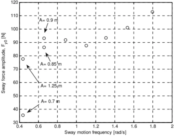
B. The sway force amplitude
It is simplest first to interpret the results for a single bare-hull configuration, and then the effect of model size can be studied. Sway force amplitude versus sway frequency for LDR 8.5 is plotted in Fig. 4. It is clear that for the runs of equal frequency, the lower maximum sway velocity – that is the smaller manoeuvre amplitude – produces a smaller force. Next, the sway force amplitude is plotted against sway acceleration amplitude in Fig. 5. The run with the lowest maximum acceleration results in the smallest sway force amplitude. It is seen that the amplitude of the sway force increases with increasing amplitude of the sway acceleration. 0.4 0.6 0.8 1 1.2 1.4 1.6 1.8 2 30 40 50 60 70 80 90 100 110 120
Sway motion frequency [rad/s]
S w ay f or c e am pl it ude, Fy0 [N ] A= 1.25 m A= 0.7 m A= 0.9 m A= 0.85 m 0.1 0.2 0.3 0.4 0.5 0.6 0.7 0.8 0.9 1 1.1 30 40 50 60 70 80 90 100 110 120
Sway acceleration amplitude [m/s2]
S w ay f orc e am pl it ud e, Fy0 [N ]
Fig. 4. Sway force amplitude versus sway frequency for the bare-hull with LDR 8.5
Fig. 5. Sway force amplitude versus sway acceleration amplitude for the bare-hull with LDR 8.5
C. Phase lag between the sway force and sway velocity signals
The values of the phase lag between the sway force and sway velocity signals (minus 90 degrees) as presented in Table I for the five bare-hulls, are shown in Fig. 6. As the sway frequency, and thus the amplitude of the acceleration increase, the phase lag decreases. Also, the phase lag for longer bare-hulls is smaller. As a result, one may anticipate that if this trend continues for higher frequencies that this phase lag will tend to zero.
D. The inertial and damping terms
As was explained in section III, it is assumed that the recorded hydrodynamic loads during these pure sway runs were not affected by any free-surface effect because of the large distance from the bare-hull to the free surface. Also, it is assumed that the hydrodynamic loads due to the supporting struts did not affect the recorded signals. Thus, the recorded sway force signal is assumed to be solely due to the lateral accelerations of the bare-hull models. As is shown in Table I and Fig. 6, the sway force signal has a phase lag of φF, larger than
π/2, relative to the velocity signal. In Fig. 7 the sway velocity is shown by a vector pointing to the right, the sway acceleration vector points upward, and the sway force vector is shown in the second quadrant. Since with increasing time these vectors rotate in the clockwise direction, the velocity vector leads the sway force vector by the angle φF. Projecting this sway force vector along the real and
imaginary axes respectively produces (i) the damping component of the force vector, named Fy,d, which acts in phase with the velocity
vector but in the opposite direction, and, (ii) the inertial component of the force vector, named Fy,i, which is in phase with the acceleration
vector.
a
yv
F
y0, iF
y0F
y0, dφ
FRe
Im
Fig. 7. Velocity, acceleration and force vectors in the complex plane
55 60 65 70 0.4 0.6 0.8 1 1.2 1.4 1.6 1.8 2 35 40 45 50
Sway motion frequency [rad/s]
P has e lag bet w S w ay v el oc it y s ignal een t he f or c e and s m inus 90 [deg] LDR 8.5 LDR 9.5 LDR 10.5 LDR 11.5 LDR 12.5
Fig. 6. Phase lag between the sway force and sway velocity signals (minus 90 degrees) during pure sway runs
As shown in Fig. 7 the amplitude of the damping and inertial components of the sway force vector are derived as:
Fy0, d = −Fy0 sin(φF − π/2) (5)
Fy0, i = Fy0 cos(φF − π/2) (6)
According to the experimental data in Table I and Fig 6, as the frequency increases (i) the magnitude of the sway force increases and (ii) the phase lag φF decreases, both of which result in a larger inertial component of the sway force.
E. The apparent mass versus manoeuvring frequency and amplitude
If the inertial component of the sway force vector in (6) is divided by the amplitude of the sway acceleration, the resulting parameter is the apparent mass of the system (the flooded vehicle mass plus the added mass of the surrounding water external to the vehicle), that is:
Fy0, i / ay0 = mapparent[kg] (7)
where ay,0 is given by A·ω2. The magnitude of the apparent mass from (7) is shown in the second last column in Table I for all
pure sway runs for all the bare-hulls. The apparent mass for the bare-hull with LDR 8.5 is plotted in Fig. 8 versus the sway acceleration amplitude. The same data are plotted versus the sway frequency ω and amplitude A in Figs. 9 and 10. The sway velocity amplitude for each data point is also shown in Figs. 8 to 10.
0.4 0.6 0.8 1 1.2 1.4 1.6 1.8 75 80 85 90 95 100 105 110 115 120 125
Sway motion frequency [rad/s]
A pparent m as s [ k g] v0= 0.57 m/s v0= 0.55 m/s v0= 0.58 m/s v0= 0.60 m/s v0= 0.55 m/s v0= 0.56 m/s v0= 0.31 m/s 0.1 0.2 0.3 0.4 0.5 0.6 0.7 0.8 0.9 1 1.1 75 80 85 90 95 100 105 110 115 120 125
Sway acceleration amplitude [m/s2]
A pparent m as s [ k g] v0= 0.58 m/s v0= 0.56 m/s v0= 0.55 m/s v0= 0.55 m/s v0= 0.60 m/s v0= 0.57 m/s v0= 0.31 m/s
Fig. 9. Apparent mass of the bare-hull with LDR 8.5 versus sway frequency during pure sway runs
Fig. 8. Apparent mass of the bare-hull with LDR 8.5 versus sway acceleration amplitude during pure sway runs
0.3 0.4 0.5 0.6 0.7 0.8 0.9 1 1.1 1.2 1.3 75 80 85 90 95 100 105 110 115 120 125
Sway motion amplitude [m]
A pparent m as s [ k g] v0= 0.57 m/s v0= 0.55 m/s v0= 0.58 m/s v0= 0.31 m/s v0= 0.55 m/s v0= 0.60 m/s v0= 0.56 m/s
Fig. 10. Apparent mass of the bare-hull with LDR 8.5 versus sway amplitude during pure sway runs
Clearly seen for the LDR 8.5 data, the apparent mass resulting from these lateral acceleration manoeuvres is variable. From Figs. 8 to 10 the following conclusions can be made:
1. Fig. 8 shows that as the amplitude A·ω2
of the sway acceleration increases, the apparent mass decreases. 2. Fig. 9 shows that as the frequency ω of the sway motion increases, the apparent mass decreases. 3. Fig. 10 shows that as the amplitude A of the sway motion increases, the apparent mass increases.
4. According to Fig. 8, the lateral velocity and acceleration have independent effects on the magnitude of the apparent mass, because the data with different sway velocity amplitudes do not lie along a curve. Since the velocity and acceleration amplitudes are respectively: A·ω and A·ω2
, it can be concluded that the oscillation amplitude and frequency are in fact the two independent factors that are affecting the magnitude of the apparent mass besides the body geometry, that is:
mapparent= f (A, ω, geometry) (8)
5. In Fig. 9 for the same sway velocity 0.55 m/s, the three data-points which have frequencies higher than 1 rad/s result in almost the same apparent mass of about 85 kg.
6. According to Fig. 10, for the same sway motion amplitude, a lower sway velocity amplitude A·ω results in larger apparent mass. Note that one should avoid concluding from the two smallest frequency data-points in Fig. 9 that for the same frequency a larger amplitude of the sway velocity results in a larger apparent mass, because then the next pair of data-points in Fig. 9, which also have the same frequency suggest the contrary. Thus, again it is emphasized that for equal motion amplitude, according to Fig. 10, a sway manoeuvre with a longer period results in a larger apparent mass. 7. From Fig. 10 one should not conclude that the magnitude of the apparent mass will indefinitely increase as the amplitude
of the sway motion increases. The apparent mass will reduce to the vehicle mass for large amplitudes. Because, for an arbitrary sway velocity amplitude, if the oscillation amplitude becomes too large, then the sway acceleration amplitude tends to zero. The reason is that the sway acceleration amplitude is as follows:
ω= v0/ A, and a0= A· ω2 → a0= v02/ A (9)
Thus, for an arbitrary sway velocity if the sway motion amplitude becomes too large, then the sway acceleration becomes so small that the inertial effects notably vanish.
8. The flooded vehicle mass for LDR 8.5 was measured to be about 49.2 kg [Hewitt and Waterman, 2005] by which amount the data in Figs. 8 to 10 should be shifted downward to show the added mass values; that is, the added mass for LDR 8.5 varies between about 28.3 to 71.2 kg depending on the sway frequency and amplitude.
F. The apparent mass versus the bare-hull size
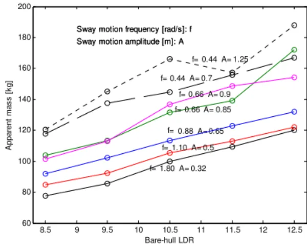
Next, Fig. 11 shows the apparent mass for the five bare-hull configurations versus the sway frequency. The clear pattern is that for all configurations the magnitude of the apparent mass appears to tend asymptotically to a single value as the frequency increases. On the other hand, if the experimental data are plotted versus the bare-hull LDR, as shown in Fig. 12, it is seen that there is effectively a linear increase in the magnitude of the apparent mass with increasing LDR, for all the combinations of sway frequency and amplitude shown.
0.4 0.6 0.8 1 1.2 1.4 1.6 1.8 2 60 80 100 120 140 160 180 200
Sway motion frequency [rad/s]
A pparent m as s [ k g] LDR 8.5 LDR 9.5 LDR 10.5 LDR 11.5 LDR 12.5 8.5 9 9.5 10 10.5 11 11.5 12 12.5 60 80 100 120 140 160 180 200 f= A= 1.80 0.32 f= A= 1.10 0.5 f= 0.88A= 0.65 f= A= 0.44 0.7 f= A= 0.66 0.85 f= A= 0.66 0.9 f= A= 0.44 1.25 Sway motion frequency [rad/s]: f
Sway motion amplitude [m]: A
Bare-hull LDR A p pa re nt m a s s [ k g ]
Sway motion frequency [rad/s]: f Sway motion amplitude [m]: A
Fig. 11. Apparent mass versus sway motion frequency for all the Fig. 12. Apparent mass versus bare-hull LDR for several combinations of sway frequency and amplitude during pure sway runs bare-hulls during pure sway runs
G. The damping factor
Going back to Fig. 5 and equation (5), if the real component of the sway force vector, i.e. the damping component, is divided by the sway velocity amplitude the resulting value is a damping factor which is often denoted by b, that is:
|Fy0, d|/ v0 = b [kg/s], where: v0= A· ω (10)
0.4 0.6 0.8 1 1.2 1.4 1.6 1.8 2 100 110 120 130 140 150 160 170 180 190
Sway motion frequency [rad/s]
D am pi n g f ac tor [ k g/ s ] LDR 8.5 LDR 9.5 LDR 10.5 LDR 11.5 LDR 12.5
Fig. 13. Damping factor versus frequency of sway motion for all bare hulls during pure sway runs
The magnitude of the damping factor from (10) is shown in the last column in Table I for all pure sway runs for all the bare-hulls. Note that the damping force acts in the opposite direction of the velocity vector, but the damping factor is defined to be positive. The damping factor derived by (10) has the dimension of [kg/s] and the dimensional values are between about 100 to 180 [kg/s]. Fig. 13 shows how the damping factor varies with the frequency of the sway motion. It is observed that the damping factor is largest for the longest model.
V. THE SWAY FORCE MODEL
Using the rotating vector representation in Fig. 7, the sway force in a pure sway manoeuvre at time instant t= 0 second can be modeled as follows:
Fy(t=0) = Fy0, d + i Fy0, i = − bv0 + i (mapparent ay0) (11)
where i is the imaginary unit vector. Equation (11) is rewritten as follows:
Fy(t=0) = − b Aω + i (mapparent Aω2) (12)
Then the amplitude of the sway force is found to be:
Fy0 = Aω [b2 + (mapparentω)2] (1/2) (13)
and the amount by which the sway force lags the sway velocity is given by:
φF = atan[−mapparentω/ b] = atan[b/ (mapparentω)] + π/2 (14)
In general, the magnitude of the apparent mass and the magnitude of the damping factor depend on the body geometry as well as the sway frequency and amplitude. The parameters for the sway force model can be obtained from the experimental data for each of the five models using (13) and (14). The time variation of the sway force is obtained by substituting the force amplitude and phase lag from (13) and (14) into equation (4), that is: Fy = Fy0 cos(ωt + φF).
VI. AN IMPROVED DESIGN FOR FUTURE PURE SWAY EXPERIMENTS
Observation of the pure sway test data revealed that the sway force vector, in addition to the body geometry, is a function of two independent variables (i) the amplitude of the sway velocity A·ω, and, (ii) the amplitude of the sway acceleration A·ω2
, in a lateral harmonic manoeuvre. In other words, the sway motion amplitude A and frequency ω should vary independently during the experiments so as to acquire data-points at different levels of both sway velocity and sway acceleration. With the present test data, since the sway amplitude and frequency had a reciprocal relation for most of the runs, it is only possible to observe the sway force variation versus lateral acceleration for a particular sway velocity amplitude of about 0.55 m/s. With a statistical design of experiment, using the concept of response surface models, the tests can be designed starting with a basic two-level factorial scheme which is then augmented with axial and centre-point runs so as to capture the variation of the response, sway force, over the two test factors: (i) the amplitude of the sway velocity A·ω, and, (ii) the amplitude of the sway acceleration A·ω2.
Fig. 14 proposes an example test plan which covers a range of 0.3 to 0.6 [m/s] for the sway velocity amplitude and a range of 0.1 to 0.8 [m/s2] for the sway acceleration amplitude. In the figure the factor sway velocity varies horizontally, and the factor sway acceleration is along the vertical axis. The design has both axial runs which are outside the square-box, and face-centered runs which lie on the sides of the square. Such an experimental plan can capture the variation of the sway force over the manoeuvring frequency and amplitude. In Table III the proposed test runs are shown; for each run the manoeuvring frequency is obtained by dividing the acceleration amplitude by the velocity amplitude, and then the amplitude A of the sway displacement equals the amplitude of the sway velocity A·ω divided by the sway frequency ω.
The centre-point run has the velocity and acceleration amplitude pair of (0.45 m/s, 0.45 m/s2) which corresponds to a frequency and sway motion amplitude of (ω, A) = (1 rad/s, 0.45 m). This run could be replicated three times so as to provide a measure of the experimental repeatability. For example, with three replications for the centre-point run, the design scheme in Fig. 14 totals to
15 runs; to this if a study of the effect of the bare-hull geometry is added, e.g. with three different bare-hulls the test set totals to 45 runs.
TABLE III. TEST-PLAN PROPOSED FOR FUTURE PURE SWAY TESTS IN
ORDER TO COVER BOTH THE MANOEUVRING FREQUENCY AND AMPLITUDE
EFFECTS ON THE SWAY FORCE RESPONSE
a0 [m/s2] Axial runs Run No. v0 [m/s] a0 [m/s2] ω= a0/ v0 [rad/s] A= v0/ ω [m] 1 0.37 0.25 0.68 0.55 2 0.53 0.25 0.47 1.12 3 0.37 0.65 1.76 0.21 4 0.53 0.65 1.23 0.43 5 0.45 0.1 0.22 2.03 6 0.45 0.8 1.78 0.25 7 0.3 0.45 1.50 0.20 8 0.6 0.45 0.75 0.80 9 0.45 0.45 1.00 0.45 10 0.45 0.25 0.56 0.81 11 0.45 0.65 1.44 0.31 12 0.37 0.45 1.22 0.30 13 0.53 0.45 0.85 0.62 VII. CONCLUSIONS
This study presents test results that indicate how the apparent mass of the bare hull of an AUV varies during a lateral acceleration manoeuvre. In oscillating lateral motions such as the pure sway manoeuvres performed in these experiments, the value of the apparent mass depends on the manoeuvring frequency and amplitude as well as the body geometry. However, the presented results indicate that further experimental and analytical research is required to acquire an improved understanding of the apparent mass and damping phenomena in lateral acceleration manoeuvres.
The sway force that is exerted on axi-symmetric bare-hull of an underwater vehicle during pure sway manoeuvres was modeled in the complex plane with its damping component in phase with sway velocity vector (but in the direction opposite to it), and its inertial component in phase with the sway acceleration vector. Then the amplitude and phase of the sway force were formulated versus the manoeuvring frequency and amplitude, the magnitude of the apparent mass and the magnitude of the damping factor of the system. As mentioned, it was shown that the magnitude of the apparent mass itself is a function of the body geometry, and the manoeuvring frequency and amplitude.
From these results, it can be deduced that for a zigzag manoeuvre also the value of the apparent mass and apparent moment of inertia may depend on the manoeuvring amplitude and frequency as well as the body geometry. For the zigzag manoeuvring tests that were performed on these bare-hull models, in a future report the effect of the apparent mass and apparent moment of inertia will be discussed. Also, an improved test-plan for future experimental work was proposed in section VI so that to perform the pure sway tests in a way that both the manoeuvring frequency and amplitude effects on the response sway force are independent variables instead of their product A·ω being effectively held constant as is shown in the fourth column of Table I for the present experiments.
ACKNOWLEDGMENT
The authors gratefully acknowledge: the Memorial University, the Institute for Ocean Technology, National Research Council Canada (NRC-IOT) and the National Science and Engineering Research Council (NSERC) for their technical, intellectual and financial support of this research.
REFERENCES
[1] C.D. Williams, T.L. Curtis, J.M. Doucet, M.T. Issac, F. Azarsina, “Effects of Hull Length on the Manoeuvring Characteristics of a Slender Underwater Vehicle,” OCEANS'06 MTS/IEEE-Boston Conference, September 18 to 21, 2006
[2] Hewitt, G. and Waterman, E., "Phoenix Model Measurement and Bifilar Swinging", NRC-IOT Report SR-2005-29, December 2005
v0 [m/s] (0.53, 0.65) (0.53, 0.25) (0.37, 0.65) (0.37, 0.25) (0.53, 0.45) (0.45, 0.8) (0.45, 0.65) (0.45, 0.45) (0.3, 0.45) (0.37, 0.45) (0.6, 0.45) (0.45, 0.25) Face-centred runs (0.45, 0.1)
Fig. 14. Test runs: pairs of factor levels for the sway velocity and sway acceleration amplitudes
TABLE I. PURE SWAY TEST RESULTS FOR THE FIVE BARE-HULL SERIES LDR A [m] ω [rad/s] v0 [m/s] a0 [m/s2] Fy0 [N] φ[deg] F− 90 mapparent [kg] b [kg/s] 8.5 0.32 1.8 0.57 1.03 112.8 44.9 77.5 138 8.5 0.36 1.53 0.55 0.85 101 46.3 82.5 132 8.5 0.42 1.31 0.55 0.72 93.3 49.7 83.8 130 8.5 0.5 1.1 0.55 0.61 87.5 53.9 84.9 128 8.5 0.65 0.89 0.58 0.51 91.8 59.4 91.8 137 8.5 0.7 0.44 0.31 0.14 35.4 63.3 117.6 103 8.5 0.85 0.66 0.56 0.37 86.1 63.4 103.8 137 8.5 0.9 0.66 0.60 0.39 93.1 64.6 101.4 141 8.5 1.25 0.44 0.55 0.24 77.6 68 120.4 131 9.5 0.32 1.8 0.57 1.03 124.3 44.8 85.5 152 9.5 0.36 1.53 0.55 0.85 111.8 46.4 91.2 147 9.5 0.42 1.31 0.55 0.72 100.9 49.4 91.3 139 9.5 0.5 1.1 0.55 0.61 93.4 53.2 92.1 136 9.5 0.65 0.89 0.58 0.51 98.2 58 102.2 145 9.5 0.7 0.44 0.31 0.14 39.9 62.2 137.6 115 9.5 0.85 0.66 0.56 0.37 92.5 62.9 113.5 146 9.5 0.9 0.66 0.60 0.39 99.9 63.6 113 150 9.5 1.25 0.44 0.55 0.24 91.2 67.4 145 153 10.5 0.32 1.8 0.57 1.03 138.9 42.2 99.8 162 10.5 0.36 1.53 0.55 0.85 125.1 42.8 108.7 154 10.5 0.42 1.31 0.55 0.72 112 46.8 106.6 148 10.5 0.5 1.1 0.55 0.61 103.5 51.8 105.3 148 10.5 0.65 0.89 0.58 0.51 107.5 57.5 113.4 158 10.5 0.7 0.44 0.31 0.14 42.6 62.7 144.5 123 10.5 0.85 0.66 0.56 0.37 102.4 61.4 131.6 160 10.5 0.9 0.66 0.60 0.39 108.6 60.3 136.7 158 10.5 1.25 0.44 0.55 0.24 95.1 65 166.2 157 11.5 0.32 1.8 0.57 1.03 148.9 40.7 109.4 169 11.5 0.36 1.53 0.55 0.85 132.7 42.7 115.4 163 11.5 0.42 1.31 0.55 0.72 119.7 45.9 115.7 156 11.5 0.5 1.1 0.55 0.61 111.3 52 112.8 159 11.5 0.65 0.89 0.58 0.51 113.7 56.7 122.7 165 11.5 0.7 0.44 0.31 0.14 44.4 61.7 155.9 127 11.5 0.85 0.66 0.56 0.37 104.1 60.2 139 161 11.5 0.9 0.66 0.60 0.39 112.7 58.7 148.6 162 11.5 1.25 0.44 0.55 0.24 99.1 67.4 157.4 167 12.5 0.32 1.8 0.57 1.03 160.7 39.6 120.1 178 12.5 0.36 1.53 0.55 0.85 144.8 40.8 129.6 172 12.5 0.42 1.31 0.55 0.72 130 42.8 132.7 161 12.5 0.5 1.1 0.55 0.61 116.6 50.5 122.1 163 12.5 0.65 0.89 0.58 0.51 118 55.3 131.9 169 12.5 0.7 0.44 0.31 0.14 44.2 59.3 167 124 12.5 0.85 0.66 0.56 0.37 121.3 58.2 172 183 12.5 0.9 0.66 0.60 0.39 118.4 59.2 154 171 12.5 1.25 0.44 0.55 0.24 103.8 64.1 188.1 170


![TABLE I. P URE S WAY T EST R ESULTS FOR THE F IVE B ARE- H ULL S ERIES LDR A [m] ω [rad/s] v 0 [m/s] a 0 [m/s 2 ] F y0 [N] φ F − 90 [deg] m apparent [kg] b [kg/s] 8.5 0.32 1.8 0.57 1.03 112.8 44.9 77.5 138 8.5 0.36 1.53 0.55 0.85 101 4](https://thumb-eu.123doks.com/thumbv2/123doknet/14168733.474276/10.918.202.719.120.1061/table-ure-way-est-esults-ive-eries-apparent.webp)
