Publisher’s version / Version de l'éditeur:
Applied Soft Computing, 11, 8, p. 4971–4980, 2011-12-01
READ THESE TERMS AND CONDITIONS CAREFULLY BEFORE USING THIS WEBSITE. https://nrc-publications.canada.ca/eng/copyright
Vous avez des questions? Nous pouvons vous aider. Pour communiquer directement avec un auteur, consultez la Questions? Contact the NRC Publications Archive team at
[email protected]. If you wish to email the authors directly, please see the first page of the publication for their contact information.
NRC Publications Archive
Archives des publications du CNRC
This publication could be one of several versions: author’s original, accepted manuscript or the publisher’s version. / La version de cette publication peut être l’une des suivantes : la version prépublication de l’auteur, la version acceptée du manuscrit ou la version de l’éditeur.
For the publisher’s version, please access the DOI link below./ Pour consulter la version de l’éditeur, utilisez le lien DOI ci-dessous.
https://doi.org/10.1016/j.asoc.2011.06.003
Access and use of this website and the material on it are subject to the Terms and Conditions set forth at
An Evolutionary Framework Using Particle Swarm Optimization for
Classification Method PROAFTN
Al-Obeidat, Feras; Belacel, Nabil; Carretero, Juan A.; Mahanti, Prabhat
https://publications-cnrc.canada.ca/fra/droits
L’accès à ce site Web et l’utilisation de son contenu sont assujettis aux conditions présentées dans le site LISEZ CES CONDITIONS ATTENTIVEMENT AVANT D’UTILISER CE SITE WEB.
NRC Publications Record / Notice d'Archives des publications de CNRC:
https://nrc-publications.canada.ca/eng/view/object/?id=ab0d4beb-dfd6-4ec8-97e3-2f052515ccdd https://publications-cnrc.canada.ca/fra/voir/objet/?id=ab0d4beb-dfd6-4ec8-97e3-2f052515ccdd
An Evolutionary Framework Using Particle Swarm
Optimization for Classification Method PROAFTN
Feras Al-Obeidat∗,a, Nabil Belacela,c, Juan A. Carreterob, Prabhat Mahantic
aInstitute of Information Technology, National Research Council, NB, Canada
bDepartment of Mechanical Engineering, University of New Brunswick, Fredericton, NB, Canada cDepartment of Computer Science, University of New Brunswick, Saint John, NB, Canada
Abstract
The aim of this paper is to introduce a methodology based on the particle swarm optimization (PSO) algorithm to train the Multi-Criteria Decision Aid (MCDA) method PROAFTN. PSO is an efficient evolutionary optimization algorithm using the social behavior of living organisms to explore the search space. It is a rela-tively new population-based metaheuristic that can be used to find approximate solutions to difficult optimization problems. Furthermore, it is easy to code and robust to control parameters. To apply PROAFTN, the values of several parame-ters need to be determined prior to classification, such as boundaries of intervals and weights. In this study, the proposed technique is named PSOPRO, which utilizes PSO to elicit the PROAFTN parameters from examples during the learn-ing process. To test the effectiveness of the methodology and the quality of the obtained models, PSOPRO is evaluated on 12 public-domain datasets and com-pared with the previous work applied on PROAFTN. The computational results demonstrate that PSOPRO is very competitive with respect to the most common classification algorithms.
Key words: Knowledge Discovery, Particle Swarm Optimization, MCDA, PROAFTN, Classification.
∗Corresponding author
Email addresses: [email protected] (Feras Al-Obeidat ),
[email protected] (Nabil Belacel ), [email protected] (Juan A. Carretero ), [email protected] (Prabhat Mahanti )
1. Introduction
The classification problem consists of using some known objects, usually de-scribed by a large set of vectors. Each vector is composed of a set of attributes and a class label, where the latter represents the category of the objects. The classifi-cation procedures require the development of a classificlassifi-cation model that identifies the behaviors of the available objects to recommend the assignment of unknown objects to predefined classes [4, 27, 43]. For instance, in medical diagnosis, pa-tients are assigned to disease (positive or negative) classes according to a set of symptoms.
In recent years, the most common approaches to address the classification problem have been from the fields of Artificial Intelligence/machine learning [35, 50] and Multi-Criteria Decision Aid (MCDA) [39, 54]. Machine learning algo-rithms are designed to learn a function which maps a large vector of attributes into one of several classes. The learning procedure is performed by working on a set of input-output objects called training datasets, which are used to find a function that assigns these training examples to those classes to which they really belong. After the learning process, the induced classification model is used by the algorithm to classify a new, unknown object (testing dataset) into one of the predefined classes. Some examples of common machine learning algorithms are Decision Tree (C4.5), Naive Bayes (NB), Support Vector Machine (SVM), Neu-ral Networks (NN), k-nearest neighbor (k-nn), instance-based learning, inductive logic programming, reinforcement learning, and PART [51].
MCDA methods are formal approaches which help in making decisions and evaluations mainly in terms of choosing, ranking or sorting/classifying the alter-natives [48]. MCDA methods have been widely used in many research fields; they are categorized into three fields: (1) Value measurement models (AHP [26] is a well known method belonging to this category); (2) Goal, aspiration and reference level models (Goal programming [12] is an example of this group); and finally (3) Outranking models (ELECTRE [20], PROMETHEE [49] and PROAFTN [9] are the methods that belong to this group).
MCDA [39] is another paradigm to address classification problems (a.k.a. nominal sorting problems). In MCDA, the problem of assigning objects to prede-fined classes is known as a multiple criteria classification problem (MCCP) [54]. The decision problems in MCCP require a comparison between alternatives or objects based on the scores of attributes using absolute evaluations [32]. In this case, the evaluation is performed by comparing the alternatives to different pro-totypes of classes, where the category or class is assigned to the objects based on
the highest score value. Each prototype is described by a set of attributes and is considered to be a good representative of its class [30].
This study focuses on the MCCP method PROAFTN, which is introduced by Belacel [8]. PROAFTN has been applied to the resolution of many real-world practical problems such as medical diagnosis, asthma treatment, and e-Health [9, 11]. PROAFTN has several advantages; for example, it uses the MCDA paradigm and therefore can be used to gain understanding about the problem do-main. Furthermore, PROAFTN has direct techniques which enable the decision-maker (DM) to adjust its parameters. PROAFTN is also a transparent classifica-tion method, that is, the fuzzy approach enables a PROAFTN user to have access to more detailed information concerning the classification decision [9].
However, PROAFTN uses the outranking relation models for classification purposes; hence, the implementation of outranking methods in general and PROAFTN in particular is burdensome, due to the large number of parameters that the deci-sion maker (DM) must identify. That is, to apply PROAFTN, the values of several parameters need to be determined prior to classification, such as boundaries of intervals and weights. In an MCDA context, these parameters are usually depen-dant on the judgment of the DM, who sets the “boundaries” of the attributes and the weights. This approach has shortcomings, such as it is time consuming and dependant on the availability of the DM; furthermore, there is some uncertainty whether a DM can assign accurate quantitative values to these parameters in some cases (e.g., data considered in the decision problem might be vague for the DM). To overcome these limitations, an automatic approach can be used to induce the classification model from data.
Particle Swarm Optimization (PSO) is a population-based metaheuristic in-spired by the social behavior of bird flocking or fish schooling introduced by Kennedy and Eberhart in 1995 [22]. The major advantages of PSO compared with other evolutionary algorithms could be summarized as follows: a) PSO is easy to implement and there are few control parameters to be tuned, and b) PSO is conceptually simple, computationally efficient, and robust to control parame-ters [23, 31, 37]. PSO has been successfully applied in a wide range of appli-cations such as task assignment problem [40], n-queen problem [29], and power systems [52]. In the context of classification, PSO is used for enhancing the clas-sification accuracy rate of linear discriminant analysis [34]. Furthermore, it has been applied to a variety of tasks, such as the training of artificial neural net-works [14, 16, 40, 53]. PSO is also proposed in [28] as a new tool for Data Min-ing. According to [44], PSO proved to be a suitable candidate for classification tasks, as it can obtain competitive results against C4.5/J48. PSO is utilized in [24]
to handle the problem of classification of instances in multiclass databases. In the MCDA literature, PSO was proposed recently in [33] to improve the outranking method ELECTRE.
As demonstrated by most of the aforementioned applications, PSO gets bet-ter results in a fasbet-ter and more efficient way compared with other evolution-ary population-based methods. Based on this motivation and the structure of PROAFTN, PSO is proposed here for the PROAFTN method. The proposed ap-proach is named PSOPRO; it employs PSO for training and improving the effi-ciency of the PROAFTN classifier. In this perspective, the optimization model is first presented, and thereafter a PSO algorithm is used for solving it. During the learning stage, PSO uses training samples to induce the best PROAFTN pa-rameters in the form of prototypes. Then, these prototypes which represent the classification model are used for assigning unknown samples. The target is to ob-tain the set of the prototypes that maximizes the classification accuracy on each dataset.
To check the performance of the proposed approach, firstly, PSOPRO is eval-uated on 12 classification datasets commonly used to benchmark the performance of classification algorithms. Secondly, the performance of PSOPRO is compared with the previous work applied on PROAFTN [1, 2, 3]. Finally, the efficiency of PSOPRO is evaluated against six machine learning classifiers, chosen from differ-ent machine learning perspectives including: Logical/Symbolic techniques such as Decision Tree (C4.5 [38]), Statistical learning algorithms (e.g., Naive Bayes (NB [18])), Support Vector Machine (SVM [13]), Perceptron-based techniques (e.g., Neural Networks (NN) [15]), Instance-based learning (e.g., k-nearest neigh-bor (k-nn) [46]), and the rule-based classifiers such as PART [21, 51]. The com-parisons and evaluations are made on the proposed datasets by using stratified 10 fold cross-validation. The numeric comparative study shows that PSOPRO is able to provide competitive and promising results.
The rest of the paper is organized as follows: in Section 2, the PROAFTN method and PSO are briefly presented. In Section 3, the proposed approach PSO-PRO is introduced. Description of datasets, experimental results, and a compar-ative study are presented in Section 4. Finally, conclusions are summarized in Section 5.
2. Overview of the PROAFTN method and Particle Swarm Optimization (PSO)
In this section, the PROAFTN methodology and PSO structure are reviewed. Thereafter, PSOPRO, which integrates PSO and PROAFTN for solving the clas-sification problem, is introduced. A PSO algorithm is designed for obtaining PROAFTN parameters from the training dataset in (near) optimal form. During the execution of the PSO algorithm, each individual representing the prototypes (i.e., potential solutions) has to be evaluated, which means that a value indicating the suitability of presenting the classification accuracy is returned by an objective (i.e., fitness) function. More details are presented in Section 3.
2.1. PROAFTN Method
In this section the PROAFTN methodology is described. PROAFTN belongs to the class of supervised learning to solve classification problems. The follow-ing subsections describe the notations and the classification procedure used by PROAFTN.
2.1.1. Notations
The PROAFTN notations used in this paper are presented in Table 1. 2.1.2. Initialization
Let n represents a set of objects known as a training set, consider a∈ n is an object which requires to be classified; given this object a is described by a set of m attributes {g1, g2, ..., gm} and k classes {C1,C2, ...,Ck}. The different steps of the procedure are as follows:
For each class Ch, a set of Lh prototypes are determined. For each pro-totype bhi and each attribute gj, an interval [S1j(bhi), S2j(bhi)] is defined where S2j(bh
i) ≥ S1j(bhi). Two thresholds d1j(bhi) and d2j(bhi) are introduced to define the fuzzy intervals: the pessimistic interval[S1j(bhi), S2j(bhi)] and the optimistic interval [S1j(bh
i) − d1j(bhi), S2j(bhi) + d2j(bhi)].
Figure 1 depicts the representation of PROAFTN’s intervals. To apply PROAFTN, the pessimistic interval[S1
jh, S2jh] and the optimistic interval [q1jh, q2jh] [10] for each attribute in each class need to be determined, where:
q1jh= S1jh− d1jh (1a) q2jh= S2jh+ d2jh (1b)
Table 1: Notations used by PROAFTN
A Set of objects{a1, a2, ..., an} to assign to different
categories
m Set of criteria or attributes,{g1, g2, ..., gm}
Ω set of k categories or classes such as
Ω = {C1,C2, ...,Ck}, k ≥ 2
Bh Prototype set of hthcategory, where
Bh={bh
i|h = 1, ..., k, i = 1, ..., Lh}
with bhi representing the i prototype of hthcategory
B Set of all prototypes, such as B=∪kh=1Bh
[S1
j(bhi), S2j(bhi)] The interval of the prototype bhi
for each attribute gjin each class Ch
with j= 1, 2, ..., m
d1j(bh
i) and d2j(bhi) The preference thresholds belong to the prototype bhi
for each attribute gjin each class Ch
wjh The weight for each attribute gjin each class Ch
applied to:
q1jh≤ S1jh (2a)
q2jh≥ S2jh (2b)
Hence, S1jh= S1j(bhi), S2jh= S2j(bhi), q1jh = q1j(bhi), q2jh = q2j(bih), d1jh = d1j(bhi), and d2jh= d2j(bh
i). The following subsections explain the stages required to classify the object a to the class Chusing PROAFTN.
2.1.3. Computing the fuzzy indifference relation: I(a, bhi)
The initial stage of classification procedure is performed by calculating the fuzzy indifference relation I(a, bhi). The fuzzy indifference relation is based on the concordance and non-discordance principle which represents the relationship (membership degree) between the object to be assigned and the prototype [7, 10]; it is formulated as: I(a, bhi) = ( m
∑
j=1 wjhCijh(a, b h i) ) m∏
j=1 ( 1− Dijh(a, bhi)wjh ) (3)Cj(a, bhi) Indifference Indifference
1
0
Sjh2 q2jh q1jh gj(a) d1jh d2jh Strong Weak Indifference No Indifference No Sjh1Figure 1: Graphical representation of the partial indifference concordance index between the ob-ject a and the prototype bh
i represented by intervals.
where wjhis the weight that measures the importance of a relevant attribute gjof a specific class Ch: wjh∈ [0, 1] , and m
∑
j=1 wjh= 1 Cijh(a, bhi) is the degree that measures the closeness of the object a to the prototype bhi according to the attribute gj.
Cijh(a, bhi) = min{Cijh1(a, bhi),Cijh2(a, bhi)}, (4) where Cijh1(a, bhi) = d 1 j(bhi) − min{S1j(bih) − gj(a), d1j(bhi)} d1j(bh i) − min{S1j(bhi) − gj(a), 0} and Cijh2(a, bhi) = d 2 j(bhi) − min{gj(a) − S2j(bhi), d2j(bhi)} d2j(bh i) − min{gj(a) − S2j(bhi), 0} Dijh(a, bh
i), is the discordance index that measures how far the object a is from the prototype bhi according to the attribute gj. Two veto thresholds ε1j(bhi) and
ε2
j(bhi) [8], are used to define this value, where the object a is considered perfectly different from the prototype bhi based on the value of attribute gj. Generally, the determination of veto thresholds through inductive learning is risky. These values need to be obtained by an expert familiar with the problem. However, this study is focused on the automatic approach; therefore, the effect of the veto thresholds is eliminated by setting them to infinity. As a result, only the concordance principle is used, so Eq (3) is summarized by:
I(a, bhi) = m
∑
j=1
wjhCijh(a, bhi) (5)
For more illustrations, three comparative procedures between the object a and prototype bhi according to the attribute gj are obtained (Fig. 1):
• case 1 (strong indifference):
Cijh(a, bhi) = 1 ⇔ gj(a) ∈ [S1jh, S2jh]; (i.e., S1jh≤ gj(a) ≤ S2jh) • case 2 (no indifference):
Cijh(a, bh
i) = 0 ⇔ gj(a) ≤ q1jh, or gj(a) ≥ q2jh • case 3 (weak indifference):
The value of Cijh(a, bh
i) ∈ (0, 1) is calculated based on Eq. (4). (i.e., gj(a) ∈ [q1jh, S1jh] or gj(a) ∈ [S2jh, q2jh] )
Table 2 presents the performance matrix which is used to evaluate the proto-types of classes on a set of attributes. The rows of the matrix represent the pro-totypes of the classes and the columns represent the attributes. The intersection between the row i and the column j corresponds to the partial indifference relation Cijh(a, bh
i) between the prototype bhi and the object a to be assigned according to the attribute gj.
2.1.4. Evaluation of the membership degree: δ(a,Ch)
The membership degree between the object a and the class Ch is calculated based on the indifference degree between a and its nearest neighbor in Bh. The following formula identifies the nearest neighbor:
Table 2: Performance matrix of prototypes according to their partial fuzzy indifference relation with an object a.
g1 g2 ... gj ... gm
b11 C111(a, b1
1) C211 (a, b11) ... C1j1(a, b11) ... Cm11(a, b11) b12 C211(a, b1
2) C212 (a, b12) ... C2j1(a, b12) ... Cm21(a, b12) ..
. ... ... ... ... ... ...
bhi Ci1h(a, bhi) C2hi (a, bhi) ... Cijh(a, bhi) ... Cmhi (a, bhi) .. . ... ... ... ... ... ... bkL k C Lk 1k(a, bkLk) C Lk 2k(a, bkLk) ... C Lk jk(a, bkLk) ... C Lk mk(a, bkLk)
2.1.5. Assignment of an object to the class:
The last step is to assign the object a to the right class Ch; the evaluation required to find the right class is performed by applying the following decision rule:
a∈ Ch⇔δ(a,Ch) = max{δ(a,Ci)/i ∈ {1, ..., k}} (7) 2.2. Particle Swarm Optimization Algorithm
As mentioned earlier, Particle Swarm Optimization (PSO) is a population-based and adaptive optimization technique introduced by Eberhart and Kennedy in (1995) [22, 23]. The concepts of PSO is intuitively inspired by social swarming behavior of birds flocking or fish schooling.
PSO is a metaheuristic evolutionary algorithm (EA). As in the case of many EAs, during the initialization phase potential solutions are randomly generated and then keep updating until the approximate optimum is attained. Compared with Genetic Algorithms (GA), the evolution strategy in PSO is inspired from the social behavior of living organisms, whereas the concept of GA is inspired from a biological perspective, where the potential solutions are evolved based on mating and breeding of new offspring (crossover and mutation).
The information-sharing technique in PSO is different from GA. In PSO, the potential solutions, called particles, move around the multi-dimensional search space, following and tracking the current optimum particles by changing their internal velocity. In GAs, chromosomes share information with each other. So the whole population moves like a single group towards an optimal area. From the implementation perspectives, PSO is easy to implement and computationally efficient compared with other EAs algorithms [31, 37].
To illustrate the concept of PSO, consider a group of birds flocking (called population, particles, or swarm) randomly flying in the search space seeking the best solution (i.e., food source). If one particle recognizes a better point to go to, the rest of the swarm will quickly follow this particle. The particles adapt them-selves iteratively by progressing or returning stochastically toward optimal regions by updating their velocity and current position according to their own experience and that of the group. More specifically, each particle in the swarm has reposi-tory memory, which maintains and tracks iteratively the best position the particle has ever visited. Each particle in the swarm is influenced by two environmental factors: one is social behavior presented by the whole swarm, also called a global best; and the second is the personal behavior called personal best [22, 31, 37, 41]. The general procedure of PSO is outlined in Algorithm 1.
Algorithm 1 PSO Evolution Steps
Step 1: Initialization phase, Initialize the swarm Evolution phase
repeat
Step 2: Evaluate fitness of each particle
Step 3: Update personal best position for each particle Step 4: Update global best position for entire population Step 5: Update each particle’s velocity
Step 6: Update each particle’s position
until (termination criteria are met or stopping condition is satisfied)
2.2.1. Functionality of PSO
Each particle in the swarm has mainly two variables to evolve and seek the optimum position in the search space:
Position vector : xi(t) Velocity vector : vi(t)
thus, each particle xi(t) is represented by [xi1(t), xi2(t), ..., xiD(t)] where i ∈ Npop is the index number of each particle in the swarm Npop (i.e., number of particles), Drepresents the dimension of the search space and t is the iteration number.
During the evolutionary phase, each particle is drawn stochastically toward the global optimum based on the updated value of vi and the particle’s current position xi. Thus, each particle’s new position xi(t + 1) is updated using:
vi(t) xi(t) PBest i (t) (a) vi(t + 1) xi(t) PBest i (t) − xi(t) GBest(t) − xi(t) vi(t) (b) GBest(t) xi(t + 1)
Figure 2: Particles’ evolution process through updating xi(t) and vi(t + 1).
The new position of the particle is influenced by the best position it has visited (i.e., its own experience), called personal best and denoted here as PBesti (t), and the position of the best particle in its neighborhood, called the global best and represented by GBest(t). At each iteration t, the velocity vi(t) is updated based on the two best values PBesti (t) and GBest(t) using the formula,
vi(t + 1) = ϖ(t)vi(t) | {z } inertial parameters
+ τ1ρ1(PBesti (t) − xi(t))
| {z }
personal best velocity components + τ2ρ2(GBest(t) − xi(t))
| {z }
global best velocity components
(9)
whereϖ(t) is the inertia weight factor that controls the exploration of the search space. τ1 andτ2 are the individual and social components/weights, respectively, also called the acceleration constants, which change the velocity of a particle to-wards the PBesti (t) and GBest(t). ρ
1 andρ2are random numbers between 0 and 1. PBesti (t) is the personal best position of the particle i, and GBest(t) is the neigh-borhood best position of particle i. During the optimization process, particle ve-locities in each dimension d are evolved to a maximum velocity vdmax (where d = 1...D). If the velocity of the particle in any dimension exceeds the value vdmax, then the velocity in that dimension is forced to return to its limit value. Fig-ure 2 explains graphically the velocity and position update during the evolution stage.
As shown in Eq. (9), the formula is composed of three terms: the first term represents the diversification process in the search procedure, whereas the last
Algorithm 2 PSO procedure for maximizing Initialization of particles (t = 0)
for i= 1 to Npop do
Initialize xi, viand PBesti (t) end for
Optimization:
Obtain GBest(t), the particle with the best fitness value of all the particles while maximum iterations or optimal criteria is not attained do
for each particle do
Calculate particle velocity vi(t + 1) according to Eq. (9) Update particle position xi(t + 1) according to Eq. (8) end for
for each particle xido Calculate fitness value f
if f(xi) > f (PBesti (t)) in history then set PBesti (t) = xi
end if end for Get GBest(t) end while
two terms represent the intensification process. Hence, the method has a balanced mechanism to utilize diversification and intensification in the search procedure efficiently. The pseudo code of the PSO procedure is detailed in Algorithm 2. 3. Development of PSOPRO algorithm
As discussed earlier, PROAFTN requires the elicitation of its parameters S1jh, S2
jh, q1jh, q2jh, and wjhfor the purpose of classification. In the MCDA literature, there are two main approaches used to obtain these parameters: direct techniques and indirect techniques. In the direct techniques, an interactive interview with the DM for whom the problem is being solved is needed. Usually, this approach is time consuming and greatly dependant on the ability of the DM and the certainty of the provided information. On the other hand, the indirect techniques, which are based on automatic learning methods, are alternative solutions to obtain the values of these parameters from the dataset during the learning phase.
In this work, the indirect technique (an optimization-based technique) is pro-posed to get these parameters from data in optimal form. In this approach, the
nec-essary preferential information required to construct a classifier is first extracted from the set of examples known as the training set. Then, this extracted infor-mation, called prototypes, is used as a classification model for assigning the new cases (testing dataset) to the target class. Finally, the classification model is eval-uated to test the performance of the classification algorithm. This approach is widely used by most machine learning classifiers [6, 21]. As mentioned earlier, to apply PROAFTN, the intervals[S1
jh, S2jh] and [q1jh, q2jh] satisfy the constraints in Eq. (2) and the weights wjh are required to be obtained for each attribute gj in class Ch. To simplify the constraints in Eq. (2), the variable substitution based on Eq. (1) is used. As a result, the parameters d1jhand d2jhare used instead of q1jhand q2jh, respectively. Therefore, the optimization problem which is based on maxi-mizing classification accuracy providing the optimal parameters S1jh, S2jh, d1jh, d2jh and wjh, is defined here,
P: Maximize f(S1jh, S2jh, d1jh, d2jh, wjh) (10) Subject to: S1jh≤ S2jh; d1jh, d2jh≥ 0 m
∑
j=1 wjh= 1 0≤ wjh≤ 1where f is the function which calculates the classification accuracy, and n repre-sents the number of training samples used during the optimization. The procedure for calculating the fitness function f(S1
jh, S2jh, d1jh, d2jh, wjh) is described in Table 3. To solve the optimization problem presented in Eq. (10), PSO is adopted here.
Table 3: The steps for calculating the objective function f .
For all a∈ A :
Step 1: - Compute the fuzzy indifference relation I(a, bh
i) according to Eq. (5) - Evaluate the membership degreeδ(a,Ch) according to Eq. (6) - Assign the object to the class according to Eq. (7)
Step 2: - Compare the value of the new class with the true class Ch
- Identify the number of misclassified and unrecognized classified objects - Calculate the classification accuracy (i.e. the fitness value):
n C1 C2 Ck Classes g1 g2 gm Attributes S1 w Parameters q1 S2 q2 Dataset
D
Figure 3: Dimensions of PROAFTN.
The problem dimension D (i.e., the number of parameters in the optimization problem) is described as follows: Each particle x is composed of the parame-ters S1jh, S2
jh, d1jh, d2jh and wjh, for all j= 1, 2, ..., m and h = 1, 2, ..., k. Therefore, each particle in the population is composed by D= 5 × m × k real values (i.e., x D= dim(x)), which is graphically presented in Fig. 3. Because of the hierarchal structure of PROAFTN parameters, the elements for each particle position xiare updated using:
xih jd(t + 1) = xih jd(t) + vih jd(t + 1) (11) where the velocity update vi for each element based on PBesti (t) and GBest(t) is formulated as:
vih jd(t + 1) = ϖ(t)vih jd(t) +τ1ρ1(Pih jdBest(t) − xih jd(t))
+τ2ρ2(GBesth jd(t) − xih jd(t)) (12) i= 1, ..., Npop; h= 1, ..., k
j= 1, ..., m; d = 1, ..., D
Algorithm 3 demonstrates the required steps to evolve the velocity viand par-ticle position xifor each particle containing PROAFTN parameters.
Algorithm 4 illustrates the flow of the PSOPRO procedure. After the initializa-tion of the swarm of particles, where each particle is composed of the parameters
Algorithm 3 Update of viand xibased PSOPRO Require:
m- number of attributes, k- number of classes D problem dimension
τ1,τ2, andϖ control parameters PBesti (t) and GBest(t)
vmax - boundary limits for S1jh, S2jh, d1jh, d2jhand wjhin each dimension for h= 1 to k do
for j= 1 to m do for d= 1 to D do
Update vih jd for each dthelement according to Eq. (12) Update xih jd for each dthelement according to Eq. (11) end for
end for end for Return xi
(S1jh, S2jh, d1jh, d2jhand wjh) for each attribute in each class, the optimization is then implemented iteratively. At each iteration, and based on the new fitness value for each particle, the updating of the velocity and position is applied to all particles in each generation. The target solution is to obtain the best parameters to reach best classification accuracy applied on training data. After this stage, the optimal parameters represented by GBest∗ and the testing data are submitted to PROAFTN to validate the classification model. The equations (5) to (7) are used to assign unseen data.
4. Application and Analysis of the Developed Algorithm PSOPRO 4.1. Datasets Description
The proposed PSOPRO algorithm is implemented in Java and applied to 12 popular datasets: Breast Cancer Wisconsin Original (BCancer), Transfusion Ser-vice Center (Blood), Heart Disease (Heart), Hepatitis, Haberman’s Survival (HM), Iris, Liver Disorders (Liver), Mammographic Mass (MM), Pima Indians Diabetes (Pima), Statlog Australian Credit Approval (STAust), Teaching Assistant Evalu-ation (TA), and Wine. The details of the datasets’ description and their
dimen-sionality are presented in Table 4. The datasets are in the public domain and are available at the University of California at Irvine (UCI) Machine Learning Repos-itory database [5].
Algorithm 4 PSOPRO procedure Require:
NT - training data, NS - testing data, m- number of attributes,
k- number of classes
D problem dimension, assign initial values to parameters set (S1jh, S2
jh, d1jh, d2jh and wjh)
Npop,τ1,τ2,ϖ control parameters
vmax, - boundary limits for each element in D Initialization:
for i= 1 to Npop do
Initialize xi, viand PBesti (t) consisting of (S1jh, S2jh, d1jh, d2jhand wjh) Evaluate fitness value f(xi) (the classification accuracy Eq. (10)) end for
Obtain the GBest(t), which contains the best set of (S1
jh, S2jh, d1jh, d2jhand wjh) Optimization stage:
while (maximum iterations or maximum accuracy is not attained) do for each particle do
Update viand xifor each particle according to Algorithm 3 end for
for each particle do
Calculate fitness value f(xi) according to Eq. (10) if f(xi) > f (PBesti (t)) then
set PBesti (t) = xi end if
end for
Choose the particle with the best fitness among particles as the GBest(t) end while
Apply the classification:
Table 4: Dataset Description.
Dataset Instances Attributes Classes D= dim(x)
1 BCancer 699 9 2 90 2 Blood 748 4 2 40 3 Heart 270 13 2 130 4 Hepatitis 155 19 2 190 5 HM 306 3 2 30 6 Iris 150 4 3 60 7 Liver 345 6 2 60 8 MM 961 5 2 50 9 Pima 768 8 2 80 10 STAust 690 14 2 140 11 TA 151 5 3 75 12 Wine 178 13 3 195 4.2. Parameters Settings
To apply PSOPRO, the following factors are considered before applying the optimization:
• The bounds for S1
jhand S2jhvary betweenµjh− 6σjhandµjh+ 6σjh, where
µjhandσjhrepresent mean and standard deviation for each attribute in each class, respectively;
• The bounds for d1
jhand d2jhvary in the range[0, 6σjh]. • The bounds for wjhare set between 0 and 1.
These regions are defined before starting the training stage. During the optimiza-tion phase, the parameters S1jh, S2
jh, d1jh, d2jh and wjh evolve within the aforemen-tioned boundary constraints.
The following technical factors are considered for implementing PSOPRO: • The control parameters are set as follows: τ1 = 2, τ2 = 2 and the inertia
weightϖ(t) = 1. More details about setting the control values are described by Clerc and Kennedy (2002) in [17], and by van den Bergh and Engelbrecht in [47];
• The size of population is fixed at 80;
• The maximum iteration number (genmax) is fixed at 500. In this context, three termination criteria are used as stopping condition. First, if the pre-defined maximum iteration (generation) is reached. Second, if the solution (i.e., the classification accuracy) cannot be further improved after a large number of iterations (i.e., 40 iterations). Third, if the optimal solution is reached during the optimization, that is, the classification accuracy on the training set reaches 100 %.
It is worth mentioning that each application has different properties, such as a different number of attributes, instances, or classes. Furthermore, some datasets have less noise than others (e.g., some datasets are linearly separable and others are not). Therefore, the performance of PSOPRO varies from one application to another, and the choice of optimal parameters may vary as well. However, in this work the PSO parameters are fixed for all applications.
4.3. Setting of PROAFTN’s parameters
The datasets described in Section 4.1 are divided into two subsets: a training set used to obtain PROAFTN parameters:(S1jh, S2jh, d1jh and d2jh) during learning (optimization) process, and a testing set used to evaluate the performance of the PROAFTN method in terms of classification accuracy. The experimental work is performed in two stages:
1. In the first stage (before optimization), the preliminary solution is calculated based on setting initial values for S1jh, S2jh, d1jh, d2jh and wjh. The initial values for PROAFTN parameters are initially fixed as follows: S1jh, S2jhare set to µjh− 2σjh and µjh+ 2σjh, respectively. The values d1jh and d2jh are both set to 4σjh. The values of weights wjhare set initially to 1.
2. In the second stage (optimization stage), the parameters are free to evolve within the boundary constraints betweenµjh− 6σjh andµjh+ 6σjhfor S1jh and S2jh, respectively. The bounds for d1jhand d2jhvary in the range[0, 6σjh]. The values of weights wjhare free to evolve within the range 0 to 1.
4.4. Performance evaluations of PSOPRO
It was noticed that for some applications the distribution of classes is or-dered sequentially, which affects the performance of the algorithms when test-ing or traintest-ing set are used. To eliminate this issue, the evaluation of the clas-sifiers is examined based on stratified fold cross-validation. In stratified 10-fold cross-validation, each dataset is divided into ten disjointed partitioned groups
(also known as folds) containing approximately the same number of instances (i.e., ≈ n/10). Using the stratified method, each fold contains approximately (n/10)/(number of classes) from instances belonging to each class. These par-titions maintain the class distribution presented in the original dataset (stratified folds) [51].
The performance of PSOPRO is evaluated in two stages. In the first stage, PSOPRO is tested on both training and testing on each dataset. In the second stage, the PSOPRO algorithm is compared with six machine leaning classifiers. That is, the performance of PSOPRO is computed as the percentage of correctly classified testing set instances based on the best particle obtained (prototypes) during the learning (optimization) phase. Then the results provided by PSOPRO on testing data are compared to those provided by other classifiers.
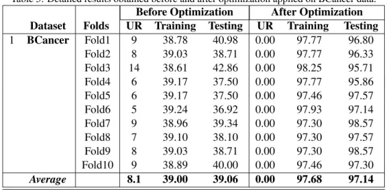
Because of the limited space and in the interest of avoiding unnecessary de-tails, the first stage of experimental work presents the detailed results on one dataset (e.g., Breast Cancer (BCancer)) presented in Table 5. The results are ob-tained on both training and testing data for each fold. As discussed above, the dataset is portioned into 10 stratified subsets and the PSOPRO algorithm is run for each partition. Each time a different set is used for testing ( i.e. 1/10 of data) and the remaining data (i.e. 9/10 of data) are used for training. This procedure is repeated until each partition of the dataset is tested. Columns 3, 4, and 5 present the preliminary solution (the results obtained before performing optimization); they are the number of unrecognized classified (UR) (i.e., the class value is not determined for the object), the result of classification accuracy based on testing data (column 4), and the result of classification accuracy based on training data (column 5). Likewise, the last three columns (6, 7, and 8) represent the same quantities, but the results are obtained after the optimization, by using PSOPRO. In the same way, Table (6) documents the same experimental procedure performed on all datasets. The only difference is that some details are omitted, such as the results for each fold. Here, the average is only documented before and after the optimization.
4.5. Comparative Study
To evaluate the performance of the proposed approach PSOPRO versus other classifiers, two comparative studies were conducted. The first study compares the performance of PSOPRO against the previous work applied on PROAFTN method [1, 2, 3]. Secondly, further experimental work was conducted with six machine learning techniques. These algorithms are chosen from different ma-chine learning theories; they are: 1) Tree induction C4.5 (J48), 2) statistical
mod-eling, Naive Bayes (NB) [18], 3) Support Vector machines (SVM) [36], SMO, 4) Function-based, Neural Network (NN), the multilayered perceptron (MLP) [42], 5) instance-based learning, IBk [46] with k= 3, and 6) rule learning, PART [45]. The open source platform Weka [51] is used to run these algorithms, using the default settings provided by Weka.
Based on Demˇsar’s recommendation [19], the Friedman test and other
ad-Table 5: Detailed results obtained before and after optimization applied on BCancer data.
Before Optimization After Optimization
Dataset Folds UR Training Testing UR Training Testing
1 BCancer Fold1 9 38.78 40.98 0.00 97.77 96.80 Fold2 8 39.03 38.71 0.00 97.77 96.33 Fold3 14 38.61 42.86 0.00 98.25 95.71 Fold4 6 39.17 37.50 0.00 97.77 95.86 Fold5 6 39.17 37.50 0.00 97.46 97.57 Fold6 5 39.24 36.92 0.00 97.93 97.14 Fold7 9 38.96 39.34 0.00 97.30 98.57 Fold8 7 39.10 38.10 0.00 97.30 97.57 Fold9 8 39.03 38.71 0.00 97.30 98.57 Fold10 9 38.89 40.00 0.00 97.46 97.30 Average 8.1 39.00 39.06 0.00 97.68 97.14
Table 6: Average results obtained before and after optimization applied on all datasets.
Before Optimization After Optimization Dataset UR Training Testing UR Training Testing 1 BCancer 8.10 39.00 39.06 0.00 97.68 97.14 2 Blood 15.3 69.79 69.78 0.00 79.94 79.25 3 Heart 0.10 58.96 59.13 0.00 86.27 84.27 4 Hepatitis 0.00 86.09 83.88 0.00 88.82 86.04 5 HM 4.60 36.08 35.22 0.00 77.66 75.73 6 Iris 1.30 64.55 65.86 0.00 97.93 96.21 7 Liver 2.60 59.09 55.61 0.00 69.34 69.31 8 MM 0.30 46.56 46.66 0.00 83.17 82.31 9 Pima 8.20 38.73 38.83 0.00 77.56 77.47 10 STAust 1.50 48.19 48.48 0.00 87.94 86.09 11 TA 0.20 47.41 46.12 0.00 58.55 60.55 12 Wine 0.00 80.59 77.33 0.00 97.76 96.79
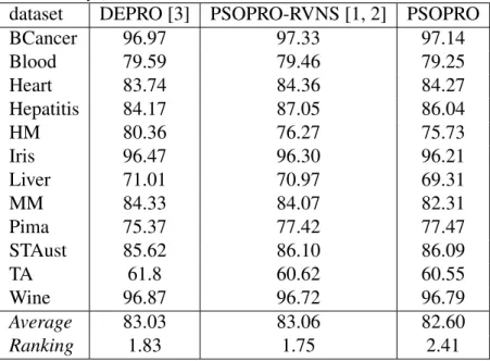
Table 7: The performance of all approaches for learning PROAFTN introduced in this thesis based on classification accuracy (in %).
dataset DEPRO [3] PSOPRO-RVNS [1, 2] PSOPRO
BCancer 96.97 97.33 97.14 Blood 79.59 79.46 79.25 Heart 83.74 84.36 84.27 Hepatitis 84.17 87.05 86.04 HM 80.36 76.27 75.73 Iris 96.47 96.30 96.21 Liver 71.01 70.97 69.31 MM 84.33 84.07 82.31 Pima 75.37 77.42 77.47 STAust 85.62 86.10 86.09 TA 61.8 60.62 60.55 Wine 96.87 96.72 96.79 Average 83.03 83.06 82.60 Ranking 1.83 1.75 2.41
vanced tests such as Bonferroni-Dunn’s, Hochberg’s, Hommel’s, and Nemenyi’s procedures described in [19] and in [25] are used to determine which classifier(s) performs the best is used to evaluate the overall performances of each classifier on all applications.
Table 7 documents the performance of PSOPRO against the previous work done on PROAFTN. In this regards, DEPRO is the abbreviation of using Differ-ential Evolution for learning PROAFTN which has been explained in [3]. The term PSOPRO-RVNS represents the utilization of PSO and Reduced Variable Neighborhood Search (RVNS) for learning PROAFTN, more details are explained in [1, 2]. For the sake of simplicity and to alleviate an extensive training load, PSO is individually used in this study for training PROAFTN parameters.
Table 8: Holm / Hochberg Table forα= 0.05
i algorithm z= (R0− Ri)/SE p Holm/Hochberg/Hommel
2 PSOPRO 1.633 0.102 0.025
1 DEPRO 0.204 0.838 0.050
Table 8 explains the performance among the the different learning methods for PROAFTN. According to the advanced statistical measures investigated here,
Bonferroni-Dunn’s procedure rejects those hypotheses that have a p-value≤ 0.025. Holm’s procedure rejects those hypotheses that have a p-value≤ 0.025, and Hom-mel’s procedure rejects those hypotheses that have a p-value≤ 0.025. Based on this outcomes, one can see that there is no significant difference in term of classi-fication accuracy between PSOPRO and PSOPRO-RVNS. Therefore, using PSO independently for PROAFTN would sufficient.
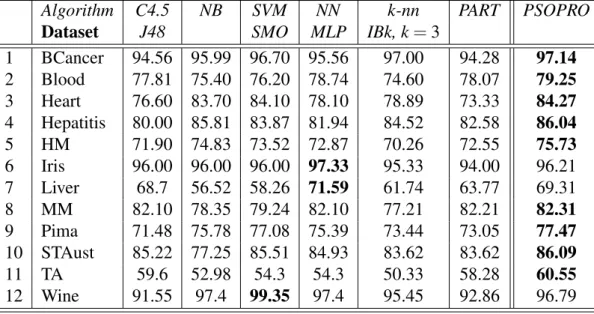
Table 9 documents the results of classification accuracy (percentage of cor-rectly classified instances) achieved by the 7 classifiers on each of the 12 appli-cations. These results are evaluated on the testing dataset and the best results achieved on each application are marked in bold. As observed from these results, PSOPRO performs very well on medical applications BCancer, Blood, Heart, Hepatitis, HM, MM and Pima.
Table 9: Experimental results based on classification accuracy (in %) to measure the performance of the different classifier compared with PSOPRO.
Algorithm C4.5 NB SVM NN k-nn PART PSOPRO
Dataset J48 SMO MLP IBk, k= 3
1 BCancer 94.56 95.99 96.70 95.56 97.00 94.28 97.14 2 Blood 77.81 75.40 76.20 78.74 74.60 78.07 79.25 3 Heart 76.60 83.70 84.10 78.10 78.89 73.33 84.27 4 Hepatitis 80.00 85.81 83.87 81.94 84.52 82.58 86.04 5 HM 71.90 74.83 73.52 72.87 70.26 72.55 75.73 6 Iris 96.00 96.00 96.00 97.33 95.33 94.00 96.21 7 Liver 68.7 56.52 58.26 71.59 61.74 63.77 69.31 8 MM 82.10 78.35 79.24 82.10 77.21 82.21 82.31 9 Pima 71.48 75.78 77.08 75.39 73.44 73.05 77.47 10 STAust 85.22 77.25 85.51 84.93 83.62 83.62 86.09 11 TA 59.6 52.98 54.3 54.3 50.33 58.28 60.55 12 Wine 91.55 97.4 99.35 97.4 95.45 92.86 96.79 The Friedman test is also used here to evaluate the overall performances of each classifier on all applications. Particularly, the focus is to evaluate whether there is a difference in the performance between PSOPRO and other classifiers. Provided that the Friedman test indicates statistically significant difference on 12 datasets and the seven classifiers including PSOPRO, other advanced tests such as Bonferroni-Dunn’s, Hochberg’s, Hommel’s, and Nemenyi’s procedures described are used to determine which classifier(s) performs the best. More particulary,
these tests are used to test whether the difference between PSOPRO versus other classifiers is meaningful. Based on the classification accuracy results obtained by each classifier presented in Table 9, the algorithms’ ranking results using Fried-man test are shown in Table 10. The best technique is the one which gives the lower value. According to these results, PSOPRO performs the best.
Table 10: Average rankings of the algorithms
Algorithm Ranking PSOPRO 1.4166 SVM 3.4583 NN 3.5416 NB 4.3750 C4.5 4.8750 PART 5.0417 3-nn 5.2917
Friedman’s and Iman-Davenport’s statistics are respectively: • Chi-square χ2= 27.8661 with 6 degrees of freedom,
• F-distribution F = 6.94537 with k − 1 and (k-1)(N-1), that is 6 and 66 de-grees of freedom.
kis the number of classifiers, and N is the number of datasets. The critical value of F(6, 66) forα= 0.05 is 2.24; this indicates that the performance of the algorithms is significantly different.
Table 11 summarizes the classifiers ordered by their p-value and the adjust-ment of α’s by Bonferroni-Dunn’s, Hochberg’s, Hommel’s, and Nemenyi’s sta-tistical procedures [19, 25]. The difference z between PSOPRO identified by R0 and other classifiers Riis presented in column 3. The standard error between two classifiers is SE =
√ k(k+1)
6N . The values are documented in the last column. p-values identify the probability of difference in performance among the classifiers over the datasets. According to this analysis, Nemenyi’s procedure rejects those hypotheses that have a p-value ≤ 0.0023. Bonferroni-Dunn’s procedure rejects those hypotheses that have a p-value ≤ 0.0083. Hochberg’s procedure rejects those hypotheses that have a p-value≤ 0.05. Hommel’s procedure rejects all hy-potheses. Based on these outcomes, the pairwise comparisons between PSOPRO and other classifiers are drawn as follows:
1. PSOPRO performs strongly better than 3-nn, PART, C4.5, and NB. 2. PSOPRO performs better than NN and SVM.
The above results show that PSOPRO is an effective classification technique that outperforms widely used classification algorithms. The fact that PROAFTN has five parameters to be obtained for each attribute for each class provides more information to assign objects to the closest class; however, in some cases this may cause some limitation on the speed of the PSOPRO. A possible future solution is to exclude the weights from learning metaheuristically using other faster and con-ceptual approaches; some techniques used in machine learning algorithms, such as features ranking, might be good choices to obtain the values of these weights without involving them in optimization. Possible improvements could be made as well on the intervals. This would involve establishing the intervals’ bounds a priori by using some clustering techniques, hence improving and speeding up the search and improving the likelihood of finding the best solutions.
5. Conclusions
In this paper, a new methodology based the evolutionary algorithm PSO is proposed for training the MCDA classification method PROAFTN. The proposed learning technique is named PSOPRO for solving classification problems. PSO is proposed to induce the classification model for PROAFTN by inferring the best parameters from data with high classification accuracy. The major properties of PSO are its ability to handle non-differentiable, nonlinear, real-valued parameters and multidimensional problems, which is the case in this work.
The performance of PSOPRO applied to 12 classification dataset demonstrates that PSOPRO outperforms the well-known classification methods PART, 3-nn, C4.5, NB, SVM, and NN. PROAFTN is a stand alone classifier algorithm which requires a technique to obtain its parameters for the studied application. PROAFTN
Table 11: PSOPRO versus other classifiers forα= 0.05 i algorithms z= (R0− Ri)/SE p 1 SVM 2.3150 0.0206 2 NN 2.4095 0.0159 3 NB 3.3544 7.9527E-4 4 C4.5 3.9213 8.8042E-5 5 PART 4.1103 3.9503E-5 6 3-nn 4.3938 1.1136E-5
uses fuzzy approach to assign objects to classes; as a result, there is richer infor-mation, more flexibility, and therefore an improved chance of assigning objects to the preferred classes. PSO is a well-known metaheuristic used successfully as a general purpose algorithm. In this study, using the PSO algorithm to obtain PROAFTN’s parameters during the learning process proved to be a successful approach for learning PROAFTN and thus greatly improving its performance.
In closing, it was observed that PSO significantly improved the performance of the PROAFTN method. Hence, the integrated approach in so-called PSOPRO demonstrates efficiency and competency in the domain of data classification. Acknowledgment
We gratefully acknowledge the support from NSERC’s Discovery Award (RGPIN293261-05) granted to Dr. Nabil Belacel.
References
[1] F. Al-Obeidat, N. Belacel, J. A. Carretero, and P. Mahanti, editors. Ad-vances in Artificial Intelligence, 23rd Canadian Conference on Artificial In-telligence, Canadian, AI 2010, Ottawa, Canada, May 31 - June 2, 2010. Proceedings, volume 6085 of Lecture Notes in Computer Science. Springer, 2010.
[2] F. Al-Obeidat, N. Belacel, J. A. Carretero, and P. Mahanti. Automatic pa-rameter settings for the proaftn classifier using hybrid particle swarm opti-mization. In Canadian Conference on AI, pages 184–195, 2010.
[3] F. Al-Obeidat, N. Belacel, J. A. Carretero, and P. Mahanti. Differential evo-lution for learning the classification method proaftn. Knowledge-Based Sys-tems, 23(5):418 – 426, 2010.
[4] E. Alpaydin. Introduction to machine learning. MIT Press, 2004.
[5] A. Asuncion and D.J. Newman. UCI machine learning repository, 2007. [6] P.W. Baim. A method for attribute selection in inductive learning
sys-tems. IEEE Transactions on Pattern Analysis and Machine Intelligence, 10(6):888–896, 1988.
[7] N. Belacel. Multicriteria Classification methods: Methodology and Medical Applications. PhD thesis, Free University of Brussels, Belgium, 1999. [8] N. Belacel. Multicriteria assignment method PROAFTN: methodology
and medical application. European Journal of Operational Research, 125(1):175–183, 2000.
[9] N. Belacel and M. Boulassel. Multicriteria fuzzy assignment method: A useful tool to assist medical diagnosis. Artificial Intelligence in Medicine, 21(1-3):201–207, 2001.
[10] N. Belacel, H. Raval, and A. Punnen. Learning multicriteria fuzzy classifi-cation method PROAFTN from data. Computers and Operations Research, 34(7):1885–1898, 2007.
[11] N. Belacel, Q. Wang, and R. Richard. Web-integration of PROAFTN methodology for acute leukemia diagnosis. Telemedicine Journal and e-Health, 11(6):652–659, 2005.
[12] D. Bouyssou, T. Marchant, M. Pirlot, P. Perny, A. Tsoukias, and P. Vincke. Evaluation and decision models. a critical perspective. Kluwer Academic Publishers, 2000.
[13] C. Burges. A tutorial on support vector machines for pattern recognition. Data Mining and Knowledge Discovery, 2(2):1–47, 1998.
[14] Xindi Cai, Nian Zhang, Ganesh K. Venayagamoorthy, and Donald C. Wun-sch, II. Time series prediction with recurrent neural networks trained by a hybrid pso-ea algorithm. Neurocomput., 70(13-15):2342–2353, 2007. [15] G. Castellano, A. Fanelli, and M. Pelillo. An iterative pruning algorithm
for feedforward neural networks. IEEE Transactions on Neural Networks, 8(3):519–531, 1997.
[16] Ying-Pin Chang and Chia-Nan Ko. A pso method with nonlinear time-varying evolution based on neural network for design of optimal harmonic filters. Expert Systems with Applications., 36(3):6809–6816, 2009.
[17] M. Clerc and J. Kennedy. The particle swarm - explosion, stability, and convergence in a multidimensional complex space. IEEE Transactions on Evolutionary Computation, 6(1):58–73, Feb 2002.
[18] G. Cooper and E. Herskovits. A bayesian method for the induction of prob-abilistic networks from data. Machine Learning, 9(4):309–347, 1992. [19] J. Demˇsar. Statistical comparisons of classifiers over multiple data sets.
Jour-nal of Machine Learning Research., 7:1–30, 2006.
[20] L. Dias, V. Mousseau, J. Figueira, and J. Climaco. An aggregation/disag-gregation approach to obtain robust conclusions with electre tri. European Journal of Operational Research, 138(2):332–348, 2002.
[21] D.M. Dutton and G.V. Conroy. A review of machine learning. The Knowl-edge Engineering Review, 12:4:341–367, 1996.
[22] R. Eberhart and J. Kennedy. New optimizer using particle swarm theory. In Proceedings of the 6th Int. Symposium on Micro Machine and Human Science, pages 39–43, 1995.
[23] R. Eberhart and J. Kennedy. Particle swarm optimization. In Proc. of the 1995 IEEE Int. Conf. on Neural Networks, volume 4, pages 1942–1948, 1995.
[24] I. De Falco, A. Della Cioppa, and E. Tarantino. Facing classification prob-lems with particle swarm optimization. Applied Soft Computing, 7(3):652 – 658, 2007.
[25] S. Garcia and F. Herrera. An extension on ”statistical comparisons of clas-sifiers over multiple data sets” for all pairwise comparisons. Journal of Ma-chine Learning Research, 9:2677–2694, 2009.
[26] Zlal Gngr, Grkan SerhadlIoglu, and Saadettin Erhan Kesen. A fuzzy ahp approach to personnel selection problem. Applied Soft Computing, 9(2):641 – 646, 2009.
[27] M. Goebel and L. Gruenwald. A survey of data mining and knowledge discovery software tools. SIGKDD Explor. Newsl., 1(1):20–33, 1999. [28] N. P. Holden and A. A. Freitas. A hybrid pso/aco algorithm for classification.
In GECCO ’07: Proceedings of the 2007 GECCO conference companion on Genetic and evolutionary computation, pages 2745–2750, New York, NY, USA, 2007. ACM.
[29] X. Hu, R.C. Eberhart, and Y. Shi. Swarm intelligence for permutation opti-mization: a case study of n-queens problem. In Swarm Intelligence Sympo-sium, 2003. SIS ’03. Proceedings of the 2003 IEEE, pages 243–246, April 2003.
[30] K. Jabeur and A. Guitouni. A generalized framework for concordance/discordance-based multi-criteria classification methods. In The 10th International Conference on Information Fusion, 2007, pages 1–8, July 2007.
[31] J. Kennedy and R.C. Eberhart. Swarm intelligence. Morgan Kaufmann Pubs., 2001.
[32] J. Lger and J-M. Martel. A multi-criteria assignment procedure for a nominal sorting problematic. European Journal of Operational Research, 138:349– 364, 2002.
[33] Karim Lidouh, Yves De Smet, and Minh Tuan Huynh. Circular representa-tions of a valued preference matrix. In Francesca Rossi and Alexis Tsoukis, editors, ADT, volume 5783 of Lecture Notes in Computer Science, pages 261–271. Springer, 2009.
[34] Shih-Wei Lin and Shih-Chieh Chen. Psolda: A particle swarm optimization approach for enhancing classification accuracy rate of linear discriminant analysis. Applied Soft Computing, 9(3):1008 – 1015, 2009.
[35] T. Mitchell. Machine Learning. McGraw Hill, 1997.
[36] S. Pang, D. Kim, and S.Y. Bang. Face membership authentication using SVM classification tree generated by membership-based lle data partition. IEEE Transactions on Neural Networks, 16(2):436–446, 2005.
[37] R. Poli. Analysis of the publications on the applications of particle swarm optimisation. Journal of Artificial Evolution and Applications, 8(2):1–10, 2008.
[38] J. R. Quinlan. Improved use of continuous attributes in C4.5. Journal of Artificial Intelligence Research, 4:77–90, 1996.
[39] B. Roy. Multicriteria methodology for decision aiding. Kluwer Academic, 1996.
[40] A. Salman, I. Ahmad, and S. Al-Madani. Particle swarm optimization for task assignment problem. Microprocessors and Microsystems, 26(8):363 – 371, 2002.
[41] Jaco F. Schutte and Albert A. Groenwold. A study of global optimization using particle swarms. J. of Global Optimization, 31(1):93–108, 2005. [42] Y. Shirvany, M. Hayati, and R. Moradian. Multilayer perceptron neural
net-works with novel unsupervised training method for numerical solution of the partial differential equations. Applied Soft Computing., 9(1):20–29, 2009. [43] P. Smyth, D. Pregibon, and C. Faloutsos. Data-driven evolution of data
min-ing algorithms. Comm. ACM, 45(8):33–37, 2002.
[44] T. Sousa, A. Silva, and A. Neves. Particle swarm based data mining algo-rithms for classification tasks. Parallel Computing, 30(5-6):767 – 783, 2004. Parallel and nature-inspired computational paradigms and applications. [45] D. K. Subramanian, V. S. Ananthanarayana, and M. Narasimha Murty.
Knowledge-based association rule mining using and-or taxonomies. Knowledge-Based Syst., 16(1):37–45, 2003.
[46] Bhekisipho Twala. Multiple classifier application to credit risk assessment. Expert Systems with Applications, In Press, Uncorrected Proof:–, 2009. [47] F. van den Bergh and A.P. Engelbrecht. A study of particle swarm
optimiza-tion particle trajectories. Informaoptimiza-tion Sciences, 176(8):937 – 971, 2006. [48] Pandian Vasant, Arijit Bhattacharya, Bijan Sarkar, and Sanat Kumar
Mukherjee. Detection of level of satisfaction and fuzziness patterns for mcdm model with modified flexible s-curve mf. Applied Soft Computing, 7(3):1044 – 1054, 2007.
[49] Xu Wei-hua, Zhang Xiao-yan, and Zhang Wen-xiu. Knowledge granulation, knowledge entropy and knowledge uncertainty measure in ordered informa-tion systems. Applied Soft Computing, 9(4):1244 – 1251, 2009.
[50] S. Weiss and C. Kulikowski. Computer Systems That Learn-Classification and Prediction methods from Statistics, Neural Nets, Machine Learning and Expert Systems. Morgan-Kaufmann, 1991.
[51] H. Witten. Data Mining: Practical Machine Learning Tools and Techniques. Morgan Kaufmann Series in Data Management Systems, 2005.
[52] H. Yoshida, K. Kawata, Y. Fukuyama, S. Takayama, and Y. Nakanishi. A particle swarm optimization for reactive power and voltage control consid-ering voltage security assessment. Power Systems, IEEE Transactions on, 15(4):1232–1239, Nov 2000.
[53] Liman Zhang, Haiming Wang, Jinzhao Liang, and Jianzhou Wang. Decision support in cancer base on fuzzy adaptive pso for feedforward neural network training. In ISCSCT ’08: Proceedings of the 2008 International Sympo-sium on Computer Science and Computational Technology, pages 220–223, Washington, DC, USA, 2008. IEEE Computer Society.
[54] C. Zopounidis and M. Doumpos. Multicriteria classification and sorting methods: A literature review. European Journal of Operational Research, 138(2):229–246, 2002.