HAL Id: halshs-01743898
https://halshs.archives-ouvertes.fr/halshs-01743898
Submitted on 26 Mar 2018
HAL is a multi-disciplinary open access
archive for the deposit and dissemination of sci-entific research documents, whether they are pub-lished or not. The documents may come from teaching and research institutions in France or abroad, or from public or private research centers.
L’archive ouverte pluridisciplinaire HAL, est destinée au dépôt et à la diffusion de documents scientifiques de niveau recherche, publiés ou non, émanant des établissements d’enseignement et de recherche français ou étrangers, des laboratoires publics ou privés.
Savage’s Theorem Under Changing Awareness
Franz Dietrich
To cite this version:
Franz Dietrich. Savage’s Theorem Under Changing Awareness. Journal of Economic Theory, Elsevier, 2018, 176, pp.1-54. �10.1016/j.jet.2018.01.015�. �halshs-01743898�
Savage’s Theorem under changing awareness
Franz Dietrich1
Final version of January 2018 for Journal of Economic Theory
Abstract
This paper proposes a simple unified framework of choice under changing aware-ness, addressing both outcome awareness and (nature) state awareaware-ness, and both how fine and how exhaustive the awareness is. Six axioms characterize an (essen-tially unique) expected-utility rationalization of preferences, in which utilities and probabilities are revised according to three revision rules when awareness changes: (R1) utilities of unaffected outcomes are transformed affinely; (R2) probabilities of unaffected events are transformed proportionally; (R3) enough probabilities ‘ob-jectively’ never change (they represent revealed objective risk). Savage’s Theorem is a special case of the theorem, namely the special case of fixed awareness, in which our axioms reduce to Savage’s axioms while R1 and R2 hold trivially and R3 re-duces to Savage’s requirement of atomless probabilities. Rule R2 parallels Karni and Viero’s (2013) ‘reverse Bayesianism’ and Ahn and Ergin’s (2010) ‘partition-dependence’. The theorem draws mathematically on Kopylov (2007), Niiniluoto (1972) and Wakker (1981). (JEL codes: D81, D83.)
Keywords: Decision under uncertainty, outcome unawareness versus state un-awareness, non-fine versus non-exhaustive un-awareness, utility revision versus prob-ability revision, small worlds versus grand worlds
1
Introduction
Savage’s (1954) expected-utility framework is the cornerstone of modern decision theory. A widely recognized problem is that Savage relies on sophisticated and stable concepts of outcomes and (nature) states: ideally, outcomes always capture everything that matters ultimately, and states always capture everything that influences outcomes of actions.2 In real life, an agent’s concepts or ‘awareness’ can
1Paris School of Economics & CNRS; fd@franzdietrich.net; www.franzdietrich.net.
2This ideal translates partly into Savage’s formal analysis: his axioms imply high state
soph-istication (i.e., infinitely many states), while permitting low outcome sophsoph-istication (i.e., possibly just two outcomes). So Savage’s formal model can handle an unsophisticated outcome concept, but neither an unsophisticated state concept, nor changing state or outcome concepts.
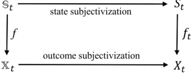
be limited at two levels, and in two ways. It can be limited at the outcome or state level, and it can be non-fine (coarse) or non-exhaustive (domain-restricted). A social planner deciding where to build a new nuclear power plant on his island has a non-exhaustive state concept if he fails to foresee some contingencies such as a tsunami. He has a non-fine state concept if he conceives a tsunami as a primitive possibility rather than decomposing it into the (sub)possibilities of a tsunami arriving from the east, west, north, or south. These are examples of state unawareness; analogous examples exist for outcome unawareness. Figure 1
c d b a z w y x c d b a z w y x c d b a z w y x f g
Figure 1: An objective act (left) and its two subjective representations (middle) and (right) under two different awareness levels (indicated by circles)
shows a situation where from an omniscient third-person perspective there are four objective states and four objective outcomes . The left-hand plot shows an objective act whose outcome is under state and is otherwise. The middle and right-hand plots show two subjective awareness levels of the agent who both times conceives only two outcomes and two states; each subjective outcome (or state) is given by a set of one or more objective outcomes (or states), indicated by a circle. In the middle plot, the agent lacks a fine awareness of outcomes and states: and are merged into the same subjective outcome, and and into the same subjective state. He also lacks an exhaustive awareness of outcomes and states: and are ignored, i.e., absent from all subjective outcomes or states. The mentioned objective act is conceived as an act mapping { } to {}, and {} to { }. In the right-hand plot, awareness is still not fine, but it is exhaustive, both at the outcome and state level. The act is now reconceived as a constant act which yields outcome { } at both subjective states { } and { }. One might compare our objective and subjective states with Savage’s (1954) grand-world and small-world states, respectively, although we allow changes in subjective states while Savage takes both types of states to be fixed.
An agent with an expected-utility rationalization does in each awareness state or context hold (i) a utility function over currently conceived subjective outcomes and (ii) a probability function over currently conceived subjective states. So in the awareness state shown in the middle of Figure 1 the agent assigns utilities only to the subjective outcomes { } and {}, and probabilities only to the subjective states { } and {}. I will consider revision rules governing the change in utilities and probabilities as the agent’s awareness or concepts chage. The first two rules
are:
R1: Utilities of preserved subjective outcomes are transformed in an increasing affine way.
R2: Probabilities of preserved subjective events are transformed proportionally. These rules are vacuous when applied to the change from the middle awareness state in Figure 1 to the right one, since no subjective outcome and only one subjective state (i.e., { }) is preserved. But now assume the middle awareness state changes differently: all existing subjective outcomes and states are preserved, and the new ones {} and {} are added. Then R2 requires the new probabilities of { } and {} to be proportional to the old ones, and R1 requires the new utilities of { } and {} to be an increasing transformation of the old ones (‘affineness’ is vacuous in case of only two preserved outcomes).
There is a clear need for a generalization of Savage’s expected-utility theory so as to cope with changes in awareness of the various sorts. If such a generalization has not yet been offered, it is perhaps because of two obstacles. One is the liter-ature’s almost exclusive focus on state unawareness; I hope to raise ‘awareness’ of outcome unawareness. Another obstacle is Savage’s high demands of state soph-istication which go against the idea of state unawareness; we will find a way to require less state sophistication, allowing for finite state spaces.
I shall offer a Savagean expected-utility (‘EU’) theory under changing aware-ness, with ‘rational’ revision of utilities and probabilities. I take the agent to be classical in all respects except from changing awareness (future research might explore non-EU preferences under changing awareness and/or boundedly rational revision rules). I work within a simple unified model of changing awareness, captur-ing changes in outcome and state awareness, and in refinement and exhaustiveness. Six axioms are then introduced, and shown to characterize an EU agent who, un-der any change in awareness, updates his utilities and probabilities according to the rules R1 and R2 and a third rule stated later. Probabilities are unique, and utilities are unique up to increasing affine rescaling. Utility revision is a genuine necessity: utilities cannot generally be scaled such that R1’s transformation is al-ways the identity transformation. The theorem generalizes Savage’s Theorem: it reduces to it in the limiting case of stable awareness, as our axioms then reduce to Savage’s axioms, while rules R1 and R2 hold trivially and the third rule reduces to Savage’s atomlessness condition on beliefs.
The framework allows for different interpretations. For instance, the agent’s awareness level could have different sources; one of them is the framing of the decision problem. Also, unawareness could be of radical and non-radical type. Radical unawareness of X is an in-principle inability to imagine or represent X. As yet unexperienced dimensions of reality or undiscovered phenomena presumably
fall under radical unawareness. Non-radical unawareness of X means that we merely do not consider X, be it because we set X aside on purpose or overlook X by mistake. Although we are in principle able to consider or understand X, we leave X aside — either because X is not worth considering due to mental costs, or because X escapes our attention due to framing or other circumstances. For instance, in a cooking choice we ignore a coin toss just because nothing hinges on it, and forget to ask how salty the dish will taste out of distraction; but we are radically unaware of tastes and flavours we have never experienced.
Choice theorists have tackled unawareness in different ways. The agent’s (un)awareness level can be an input or an output of the analysis: it can be an exogenous starting point which is assumed, or a feature which should be revealed by observed behaviour. Recent examples of the ‘revealed (un)awareness’ approach are Schipper (2013) and Kochov (2016).3 My model follows the ‘exogenous
aware-ness’ approach, just like Ahn-Ergin’s (2010) model of framed contingencies and Karni-Viero’s (2013) model of growing awareness. How does my model relate to these two seminal contributions? Working in an Anscombe-Aumann-type frame-work, Ahn-Ergin assume that each of various possible ‘framings’ of the relevant contingencies leads to a particular partition of the objective state space (repres-enting the agent’s state concept), and to a particular preference relation over those acts which are measurable relative to that partition. Under plausible axioms on partition-dependent preferences, they derive a compact EU representation with fixed utilities and partition-dependent probabilities. The systematic way in which these probabilities change with the partition implies our rule R2 (after suitable translations). Karni-Viero, by contrast, model the discovery of new acts, out-comes, and act-outcome links. They work in a non-standard framework which takes acts as primitive objects and states as functions from acts to outcomes (fol-lowing Schmeidler and Wakker 1987 and Karni and Schmeidler 1991). They char-acterize preference change under growing awareness, using various combinations of axioms. A key finding is that probabilities are revised in a reverse Bayesian way, a property once again related to our revision rule R2.
The current analysis differs strongly from Ahn-Ergin’s and Karni-Viero’s. I now mention some differences. I analyse awareness change at both levels (outcomes and states) and of both kinds (refinement and exhaustiveness), while Ahn-Ergin limit attention to changes in state refinement (with fixed state exhaustiveness and fixed outcome awareness), and Karni-Viero assume fixed outcome refinement.4 Ahn-Ergin and Karni-Viero find that only probabilities are revised, yet I find that also
3Schipper takes unawareness of an event X to be revealed via nullness of both X and X’s
negation. Kochov studies revealed unawareness of future contingencies in a dynamic setting.
4Karni-Viero do capture changes in outcome exhaustiveness, through the discovery of new
outcomes. Changes in state awareness are captured indirectly: the discovery of new acts resp. outcomes effectively renders states finer resp. more exhaustive.
utilities are revised. Ahn-Ergin and Karni-Viero introduce lotteries as primitives (following Anscombe and Aumann 1963), while I invoke no exogenous objective probabilities (following Savage 1954). Ahn-Ergin and Karni-Viero exclude the classical base-line case of ‘state sophistication’ with an infinite state space, while I allow that ‘state sophistication’ is reached sometimes, or never, or always; this flexibility is crucial for ‘generalizing Savage’.
In the background of the paper is a vast and active literature on unaware-ness (e.g., Dekel, Lipman and Rustichini 1998, Halpern 2001, Heifetz, Meier and Schipper 2006, Halpern and Rego 2008, Hill 2010, Pivato and Vergopoulos 2015, Karni and Viero 2015). I do not attempt to review this diverse body of work, ranging from epistemic to choice-theoretic studies, from static to dynamic studies, and from decision- to game-theoretic studies. The theorem’s long proof, presented in different appendices, makes use of key theorems by Kopylov (2007), Niiniluoto (1972) and Wakker (1981).
2
A model of changing awareness
2.1
Variable Savage structures
Before introducing our own primitives, I recall Savage’s original primitives: Definition 1 A Savage structure is a triple ( %) of a non-empty finite5 set (of outcomes or consequences), a non-empty set (of states), and a (preference) relation % on the set of functions from to (acts).
I replace Savage’s fixed outcome/state spaces by context-dependent ones. This leads to a family of Savage structures ( %)where ranges over an arbitrary
set of ‘contexts’. To be able to relate the subjective outcomes/states of each context to objective ones, I take each to partition (coarsen) some underlying set
of ‘objective’ outcomes, and each to partition (coarsen) some underlying set of
‘objective’ states.6 This captures the ‘objective world’ and the agent’s (changing)
awareness of it. Formally:
Definition 2 A variable Savage structure is a family of Savage structures ( %)∈ indexed by some non-empty set (of contexts), such that
• each is a partition of some set (of objective outcomes encompassed
in context ),
• each is a partition of some set (of objective states encompassed in
context ).
5Savage in fact did not impose finiteness. I add finiteness for simplicity.
An objective outcome/state simpliciter is an objective outcome/state encom-passed in at least one context.
From now on, let ( %)∈ be a given variable Savage structure. Let:
:= (acts conceived in context )
X :=set partitioned by (objective outcomes encompassed in context )
S :=set partitioned by (objective states encompassed in context )
X := ∪∈X (objective outcomes)
S := ∪∈S (objective states)
F := XS (objective acts).
The spaces and could reflect the framing at work in context . This framing
renders certain outcome/state concepts salient, e.g., through a mode of presenta-tion or a level of descriptive detail.7 The framing-based interpretation follows Ahn and Ergin (2010), extending their idea to outcome framing as well as state fram-ing. Framing is only one of many possible sources/interpretations of the agent’s concepts and hence of the spaces and ; see Section 2.3.
Here is a two-context example corresponding exactly to Figure 1: = { 0}, ={{ } {}}, ={{ } {}}, 0 ={{ } { }}, and 0 ={{ } { }};
so X = { }, S = { }, X = X0 ={ }, and S = S0 = { }.
The agent’s outcome/state spaces are non-fine in both contexts, and non-exhaustive only in context . In general, the smaller the sets in and are, the finer the
agent’s outcome/state concepts are, up to the point of singleton sets (full refine-ment); and the larger the sets X and S are, the more exhaustive these concepts
are, up to the entire sets X and S (full exhaustiveness).
When does the agent have full awareness of some type at some level?
Definition 3 The variable Savage structure ( %)∈ has
(a) exhaustive outcomes if in all contexts we have X= X,
(b) exhaustive states if in all contexts we have S = S,
(c) fine outcomes if in all contexts each outcome ∈ is singleton,
(d) fine states if in all contexts each state ∈ is singleton.
Our theorem will simplify under exhaustive states, and simplify differently under fine states. Here are examples demonstrating the flexibility of our model:
• Savage: contains a single context 0. Our variable structure reduces to a
classic Savage structure ( %) := (0 0%0). Objective outcomes and
7If the agent is presented car insurance policies in terms of their net benefit as a function of the
number (up to 10) of accidents, then contains the 11 events ‘ accidents’ for = 0 1 10, and
contains the 11 net-benefit outcomes; another context 0with a different mode of presentation
states are not needed: w.l.o.g. we can, like Savage, let and be primitive sets rather than any partitions.
• Stable outcome awareness: All contexts lead to the same outcome space = , which we may take as a primitive set rather than any partition.
One might then identify contexts with state spaces (state awareness levels); so contains the ‘possible/feasible’ state spaces and := for all ∈ .
• Stable state awareness: All contexts lead to the same state space = ,
which we may take to be a primitive set rather than a partition. One might then identify contexts with outcome spaces (outcome awareness levels), so that contains the ‘possible/feasible’ outcome spaces and := for all
∈ .
• Fully variable awareness: All logically possible awareness states occur: for all partitions of X and of S, where || ∞, there is a context ∈ in which = and = . (To allow non-exhaustive awareness,
one should extend the quantification to partitions of any non-empty subset of X or S, respectively.) This permits arbitrary ways to conceive the world. If one identifies contexts with awareness levels, becomes the set of all pairs = ( ) of a finite partition of X and a partition of S, where := and
= .
• Finite awareness: All spaces and (and so all act sets ) are finite.
The agent can only conceive finitely many things at a time.
2.2
Excursion:
preferences over subjective or objective
acts?
Some might prefer working with preferences over objective rather than subjective acts (I do not, because the objects of preferences should be things the agent can conceive, in line with my mentalistic rather than behaviouristic position on eco-nomic modelling; see Dietrich and List 2016a, 2016b). One can indeed recast each preference relation % in our variable Savage structure as one over objective acts,
more precisely over objective acts that are representable (measurable) in context : just identify a preference between two subjective acts in with a preference
between any two objective acts represented by them in context , respectively. If wished, one could thus replace the relations % on ( ∈ ) by corresponding
relations on { ∈ F : is representable in } ( ∈ ), or at least interpret the
former relations as shorthands for the latter relations. But what exactly is the subjective representation of an objective act?
Definition 4 Given a context ∈ ,
• the subjectivization of an objective outcome ∈ X, denoted , is the
),
• the subjectivization of an objective state ∈ S, denoted , is the subjective
state in containing (the assignment 7→ maps S onto ),
Definition 5 The (subjective) representation of an objective act ∈ F in a context ∈ is the unique act ∈ (if existent) which matches modulo
sub-jectivization, in that whenever 0 ∈
subjectivizes ∈ S (i.e., ∈ 0), then (0)
subjectivizes () (i.e., () ∈ (0)). An ∈ F is (subjectively) representable
in context if its representation exists.
Remark 1 (representability as measurability) Given a context ∈ ,
• under exhaustive states and outcomes, an objective act is representable if and only if it is ( )-measurable,
• in general, an objective act is representable if and only if its restriction to S
maps into X and is ( )-measurable.8
state subjectivization
outcome subjectivization
f
Figure 2: An objective act : S → X and its representation : → (note
that indeed maps S into X by Remark 2)
Remark 2 For any objective act ∈ F representable in given a context , the diagram in Figure 2 is
(i) well-defined, i.e., (S)⊆ X(a trivial condition under exhaustive outcomes),
(ii) commutative, i.e., [ ()]= () for all ∈ S.
As an illustration, consider an objective act that makes the agent rich if a coin lands heads (and poor otherwise), and that might also do many other things, such as making him sick in the event of cold weather. In context the agent conceives only ‘wealth outcomes’ and ‘coin states’: = { } and
= { }, where and are the outcomes (sets of objective
outcomes) in which he is rich or poor respectively, and and are the states (sets of objective states) in which the coin lands heads or tails respectively. Then is represented by the subjective act that maps to and
to . But if instead = { } and = {S}, the state concept no
longer captures the coin toss, and is no longer representable.
8(
)-measurability means that members of the same ∈ are mapped into the same
2.3
Three clarifying interpretive remarks
1. One can take the spaces and ( ∈ ) to represent the awareness/concepts/ontology
ascribed to the agent by the observer: they reflect how we take him to perceive the world, and hence they embody our hypothesis (or theory, stipulation, conjecture etc.) about the agent’s perception. This ascription or hypothesis could be guided by: (i) the framing of outcomes and states; or (ii) the awareness/concepts as re-ported by the agent when asked by the analyst about his current outcome/state concepts; or (iii) the modeller’s own common sense or intuition; or (iv) neuro-physiological evidence about how the context affects the cognitive system; or (v) the sort of options that are feasible in context (here and are constructed
such that all feasible options become representable as subjective acts, in a sense made precise in Section 2.7); or (vi) observed choices (among objective acts) which reveals the agent’s awareness, in a sense that can be made precise (here and
are constructed so as to be fine enough to distinguish between those objective acts between which observed choices distinguish). There is also a completely different interpretation: the spaces and could represent the agent’s real rather than
ascribed concepts in context , adopting a first-person rather than third-person perspective. The literature routinely uses (and switches between) both types of interpretation of Savage’s outcomes and states — i.e., interpretations in terms of the agent’s ascribed or real ontology, i.e., of either our assumption about his con-cepts or his real concon-cepts possibly unknown to us. Savage himself had the second interpretation in mind; he focused on rationality from a first-person perspective. By contrast, mainstream behaviourist economics favours the first interpretation, to ensure observability of all primitives.
2. By modelling subjective outcomes/states as sets of objective ones, I by no means suggest that the agent conceives outcomes/states in terms of (complex) sets. He may conceive them as indecomposable primitives. He may for instance conceive the outcome ‘having close friends’ in complete unawareness of a huge (infinite) set of underlying objective outcomes. Only our third-person perspective identifies subjective outcomes/states with sets of objective ones.
3. One can think of a context ∈ in broadly two ways. Either represents the environment (or frame, time point, decision node in a decision/game tree, ...) which triggers or causes the agent’s awareness state ( ) and preference
relation %. Or is ‘only’ an index; can then be identified with the agent’s
awareness state itself (under a minor loss of generality9), so that is a space pair
( ), where := and := . In the first case ( %)∈ captures
how awareness and preferences react causally to the environment. In the second
9The loss of generality is that preference must then be determined (fully) by awareness:
( ) = (0 0) ⇒ %=%0. This restriction is minor, since even without making it, it later
case ( %)∈ is simply a summary of all ‘possible’ or ‘feasible’
awareness-preference states ( %) of the agent; the structure ( %)∈ could then
be abbreviated as (%)∈, as each context = ( ) already encodes the spaces
:= and := .
2.4
The objective/subjective terminology and notation
We must carefully distinguish between objective and subjective descriptions. By default descriptions are subjective; so I often drop ‘subjective’. Formally:
• An objective outcome/state/act/event is a member of X / S / F = XS
/ 2S.
• A (subjective) outcome/state/act/event conceived in context (∈ ) is a member of / / = / 2.
• A (subjective) outcome/state/act/event simpliciter (without reference to a context) is a member of some / / / 2 ( ∈ ).
• The (subjective) outcome/state space in context is / .
• A (subjective) outcome/state space simpliciter is some / ( ∈ ).
• The objectivization of an event ⊆ ( ∈ ), denoted ∗, is the objective
event partitioned by ; and ∗ are said to correspond to each other.
• Events and from possibly different contexts are (objectively) equi-valent if ∗ = ∗.
• Any act ∈ ( ∈ ) induces a function on S rather than , denoted
∗ and given by ∗() := () (where is ’s subjectivization, given by
∈ ∈ ); and ∗ are said to correspond to each other.
2.5
Expected-utility rationalizations and revision rules
We can apply the classical expected-utility paradigm within each context.
Definition 6 An expected-utility (‘EU’) rationalization/representation of the variable Savage structure ( %)∈ is a system ( )∈ of non-constant
‘utility’ functions : → R and probability measures10 : 2 → [0 1] such
that
% ⇔ E( )≥ E() for all contexts ∈ and acts ∈
Our axioms will imply existence of an (essentially unique) EU rationalization ( )∈ whose utilities and probabilities obey three revision rules. The first two
of them are easily stated:
R1: Any is an increasing affine transformation of any 0 on the domain
over-lap ∩ 0.
R2: Any is proportional to any 0 on the domain overlap 2∩0.
Under R1 and R2, utilities are affinely rescaled and probabilities are proportionally rescaled where concepts are stable. So if the agent, say, splits an outcome ∈
into and , resulting in a context 0 with
0 = (\{}) ∪ { } and 0 = ,
then 0 = by R2, and utilities are essentially unchanged on \{} by R1.
R1 and R2 are in contrast with two stronger conditions that forbid revisions: R1+: Any equals any 0 on the domain overlap ∩ 0 (‘stable utilities’).
R2+: Any equals any 0 on the domain overlap 2∩0 (‘stable probabilities’).
Neither R2 nor even R2+ prevents the agent from attaching a different prob-ability to an event ⊆ conceived in a context and an objectively
equival-ent evequival-ent 0 ⊆
0 conceived in another context 0. This happens if beliefs are
description-sensitive, i.e., dependent on how objective events are perceived sub-jectively. Imagine that in context the agent conceives the fine states {} and {} and hence the event = {{} {}}, while in context 0 he conceives the coarser state { } and hence the event 0 = {{ }}. Although and 0 represent the same objective event { }, the agent might in context find unlikely on the grounds that {} and {} each appear implausible, while in context 0 finding 0
likely because he fails to analyse this event in terms of its implausible subcases.11
The following revision rule — a significant strengthening of R2 and R2+ — excludes such description-sensitivity:
R2++: If events ⊆ and 0 ⊆ 0 ( 0 ∈ ) are objectively equivalent, then
they get the same probability, i.e., ∗ = 0∗ ⇒
() = 0(0) (‘objectively
stable probabilities’).
I now give three examples. All of them assume an EU rationalization ( )∈.
The first two concern utilities, and the last one concerns probabilities.
Example 1: stable utilities. Objective outcomes are numbers between 0 and 100: X = [0 100). The agent has a coarse conception of numbers, i.e., conceives ‘vague numbers’ in the form of intervals. So each outcome space consists of
pairwise disjoint intervals. If for instance ={[ + 1) : = 0 99}, then the
agent effectively ignores decimals, i.e., identifies any numbers having the same non-decimal digits. How might he assign utilities? Suppose all utilities are reducible
11Concretely, could stand for country 1 attacking country 2, and for 2 attacking 1. In
context the agent finds event = {{} {}} unlikely: he reasons that {} and {} are each implausible as each country is unlikely to attack. In context 0, he finds event 0= {{ }} likely
on unsophisticated grounds: he treats 0 as a primitive scenario of ‘war’, which seems likely to
to a fixed utility function of objective states : X → R, in one of the following ways. For any context and any outcome ∈ (an interval),
• () = ()where is a ‘representative’ or ‘rounded’ number defined, e.g.,
as ’s lower boundary inf or upper boundary sup or midpoint inf +sup 2 ; • () = where is a ‘representative’ or ‘rounded’ utility level defined, e.g.,
as inf∈ () or sup∈ () or inf∈ ()+sup∈ ()
2 .
In all these cases utility revision satisfies not just R1, but even R1+ (stable util-ities), since ()depends only on , not on the context .12
Example 2: changing utilities. As in the previous example, let X = [0 100), and let each consist of pairwise disjoint intervals. But utilities are no longer
reducible to a fixed utility function on X. Instead they are formed as follows. In any context , the outcomes (intervals) in are put into a linear order
1 2 such that 1’s members are smaller than 2’s, which are smaller than
3’s, etc., where = ||. Let (1) = 1, (2) = 2, ..., () = . This
leads to utility revisions: for instance, the same outcome [50 100) gets utility ([50 100)) = 2 when = {[0 50) [50 100)}, but utility 0([50 100)) = 3
when 0 = {[0 10) [10 50) [50 100)}. Neither R1+ nor even R1 needs to hold:
two utility functions and 0 need not be increasing affine transformations of
one another on ∩ 0. However, R1 does hold if never more than 3 outcomes
are conceived (i.e., || ≤ 3 for all ∈ ), or never more than 4 outcomes are
conceived and outcome awareness is exhaustive (i.e., each partitions the full
interval X = [0 100)). The reason is that in these cases any two spaces 0
either share at most two elements (so that is an increasing affine transformation
of 0 on ∩ 0), or coincide (so that = 0).
Example 3: objectively stable beliefs. Let the source of uncertainty be purely objective. That is, let S contain the outcomes of some random experiment, e.g., coin tossing sequences or roulette outcomes. We capture the objective risk by a probability measure on some algebra R on S. In each context the agent conceives only finitely many states: is a finite partition of S into members of
R. (If S contains coin tossing sequences and in context only the first three tosses are conceived, then states in correspond to triples of outcomes of the first three
tosses.) Despite his limited state conception, let the agent give the true (objective) probability to those states he conceives: () = () for all contexts and states
∈ . Then clearly R2++ (and thus R2 and R2+) hold.
12Is it plausible to reduce all
s to a fixed function on X? One might object that agents
with limited awareness do not conceive the objects X and , and so cannot consciously calculate values like (inf ) or inf∈ (); the utility model would thus have an ‘as if’ status, hence
2.6
Tighter EU rationalizations and their revision rules
I now sketch tighter kinds of EU rationalizations with fewer degrees of freedom: ‘stable’, ‘unified’, and ‘classical’ EU rationalizations. In each case some of the revision rules R1, R1+, R2, R2+ and R2++ come for granted. The unified and classical cases can be linked to Ahn-Ergin’s (2010) central rationalization con-cepts.13
Stable and unified EU rationalizations. I begin with utilities, and then turn to probabilities.
Definition 7 A family ()∈ of utility functions on is stable if it is given
by a single function on ∪∈in that each matches on , i.e., = |.
Remark 3 Stability of ()∈ is equivalent to R1+, so implies R1.
Definition 8 A family ()∈ of probability functions on 2 is
• stable if it is given by a single function on ∪∈2 in that each is equal
to on 2, i.e.,
= |2,
• unified if more generally it is given by a single function on ∪∈2 in
that each is proportional to on 2, i.e., ∝ |2.14
Remark 4 Stability of ()∈ is equivalent to R2+, which implies unification,
which in turn implies R2.
Definition 9 If an EU rationalization ( )∈ is stable in its utility functions
(given by ) and stable or more generally unified in its probability functions (given by ), then ( )∈ — or in short ( ) — is a stable EU rationalization or
more generally unified EU rationalization, respectivey.15
Remark 5 An EU rationalization ( )∈ is
• stable if and only if R1+ and R2+ hold,
• unified if R1+ and R2+ hold, and only if R1+ and R2 hold.
13If Ahn-Ergin’s framework is recast within ours, it corresponds to the special case of a fixed
outcome space = and exhaustive and finite state spaces . In this case, our unified and
classical EU rationalizations reduce essentially to their dependent’ resp. ‘partition-independent’ EU representations (partly because the conditions which unification and classicality impose on the functions reduce to Ahn-Ergin’s assumption of a fixed utility function).
14Even if
is just proportional to on 2, fully determines , given that () = 1. 15One might also consider EU rationalizations which are stable only in utilities (short-hand:
Classical EU rationalizations. Stability of an EU rationalization is a big (and questionable) step towards classical rationality. But it falls short of it, as the agent can display major forms of dynamic inconsistency. For instance, as the context changes from to 0 and two old outcomes ∈ get merged into a single one
∪ ∈ 0, the utility 0(∪ ) could exceed the utilities () and () of
both suboutcomes — a ‘dynamic dominance violation’. Similarly, as two old states ∈ get merged into a single one ∪ ∈ 0, the probability 0(∪) can differ
from () + () — a ‘dynamic additivity violation’. The natural explanation of
such violations is, of course, that in context 0 the agent no longer conceives the
‘subcases’ of ∪ and ∪, as ∪ and ∪ appear as indecomposable primitives. I now define ‘classical’ EU rationalizations. They exclude any such dynamic inconsistency, and render the agent classical in all respects — except from awareness changes (imposed exogenously via the variable Savage structure). Such an ‘almost classical’ agent ranks subjective acts as if he conceived the underlying objective outcomes and states: although he evaluates subjective entities (outcomes, states and acts), he does so objectively, by taking into account the underlying objective outcomes and states. One may legitimately question the plausibility of such a hybrid agent: why should someone who can come up with objective evaluations fail to come up with objective outcomes, states and acts in the first place? The point of defining classical EU rationalizations is not to defend ‘objective evaluations of subjective objects’ as genuinely realistic, but to spell out the classical benchmark from which our less classical rationalizations depart.
Let us start with classical probabilities, before turning to classical utilities. From an orthodox rationality perspective, it should not matter how objective events are subjectively represented (described, framed), in the following sense:
Definition 10 A family ()∈ of probability functions on 2 is classical if
the probability of any event depends only on its objectivization ∗, i.e., if ( )∈
is given by a single function on the set ∪∈{∗ : ∈ 2} of objectivized events:
() = (∗) for all contexts ∈ and events ⊆
Remark 6 Classicality of ()∈ is equivalent to R2++ (objectively stable
prob-abilities), hence implies R2 and R2+.
In Example 3, ()∈ is classical, and generated precisely by the example’s
true probability measure (restricted to ∪∈{∗ : ∈ 2}).
Turning to classical utilities, imagine in a context the agent conceives the outcome { }, which has two underlying objective outcomes; { } might stand for ‘rich’, for ‘very rich’, and for ‘moderately rich’. Under the classical expected-utility paradigm, composite prospects are systematically evaluated in terms of the
expected/average utility of their subprospects. Accordingly, the prospect { } is to be evaluated in terms of the expected/average utility of and . This requires assigning utilities and probabilities to objective outcomes. Invoking probabilities at the outcome level is unconventional — but it is natural and necessary if coarse outcomes should be evaluated classically by the expected utility of the objective (sub)outcomes. This motivates the following definition:
Definition 11 A family ()∈ of utility functions on is classical if the
utility of any outcome is the expected utility (given that outcome) of the objective outcome, i.e., if
() = E(|) for all contexts ∈ and outcomes ∈ (1)
relative to some fixed utility function of objective outcomes : X → R and some fixed probability measure on (some algebra on) X.16
Remark 7 If ()∈ is classical, then it is stable (so obeys R1+), as it is given
by the single function mapping ∈ ∪∈ to E(|) (with and as in
Definition 11).
Classicality of utilities goes far beyond stability, so beyond the rule R1+. It implies a notable property (of which R1+ is the special case in which = 1):
Remark 8 Classicality of ()∈ implies that whenever the context changes from
to 0 and a new outcome ∈
0 is partitionable into old (sub)outcomes 1 ∈
, then the new utility of is a weighted average of the old utilities of 1 :
0() =P=1(|)(), with as in Definition 11.
Definition 12 If an EU rationalization ( )∈ is classical both in its
util-ity functions (given by and ) and its probabilutil-ity functions (given by ), then ( )∈ — or in short ( ) — is a classical EU rationalization.17
Remark 9 Classical EU rationalizations ( )∈ are stable (hence unified), by
Remarks 5, 6 and 7.
Classical EU rationalizations perform a universal reduction to the objective level. Yet, as mentioned, it is hard to imagine how an agent with limited aware-ness could evaluate outcomes and states as if he were aware of underlying objective
16In particular, for each ∈ ∪
∈, E( |) is defined, meaning that (1) (·|) is
well-defined, i.e., is defined and non-zero at , and (2) has a finite expectation w.r.t. (·|) (e.g., is bounded on and measurable w.r.t. the algebra on which is defined).
17One might consider EU rationalizations (
)∈ which are classical only in utilities
outcomes and states. In defence of classical EU rationalizations, one might try to interpret them in a more literal and less as-if -like way. For that purpose ima-gine all unawareness is non-radical: the agent has in principle mental access to objective outcomes and states, but for some reason (such as simplicity) conceives outcomes and states more coarsely than he could have. Yet when assigning utilit-ies/probabilities to his coarse outcomes/events he suddenly becomes sophisticated and goes down to objective outcomes/states. I leave it open whether this back-and-forth between a coarse and a fine perspective is psychologically plausible — and if not, whether an ‘as if’ interpretation is plausible. Figure 3 summarizes the
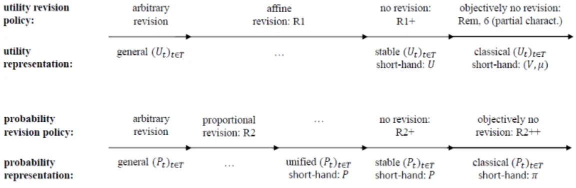
Figure 3: Revision policies for utilities/probabilities and corresponding represent-ations of utilities/probabilities, from most general (left) to most specific (right)
various revision policies with their corresponding representations, in the order of increasing specificity. I insert ‘...’ where a revision policy has no corresponding representation or where a representation has no corresponding revision policy.
2.7
Excursion: unawareness, choice behaviour, and
non-representable options
Our model is easily connected to choice behaviour. Assume the agent finds himself in a context ∈ and faces a choice between some concrete (pre-theoretic) options, such as meals or holiday destinations. The modeller faces two possibilities: he could model options either as subjective acts in or as objective acts in F. Neither
possibility is generally superior: all depends on the intended level of description. In the first case, the feasible set is a subset of , and the prediction is simply that
a most %-preferred member is chosen.
For the rest of this subsection, I assume the second case: let options be ob-jective acts. So the feasible set is a subset of F, not . Which choice does %
predict? It predicts that the agent chooses a feasible objective act whose subjective representation in (see Definition 4) is most %-preferred. More precisely, our
variable Savage structure ( %)∈ predicts that whenever in a context ∈
the agent has to choose from a set F ⊆ F of representable objective acts, then he chooses an ∈ F such that % for all ∈ F. (This may lead to choice
reversals as the context changes; see Section 4.)
No prediction is made about choice from non-representable objective acts: the model is silent on such choices. Does the model thereby miss out on many choice situations? Perhaps not, because the mental process of forming outcome/state concepts might (consciously or automatically) adapt these concepts to the feasible options, to ensure representability. I call the agent — or more exactly his awareness states ( )∈ — adaptive (to feasible options) if for each context all
objective acts that can be feasible in are representable in .18 The idea is that
the agent forms awareness of a coin toss when and because some feasible objective acts depend on it. Forming awareness is a costly mental activity, which is likely to be guided by the needs of real choice situations, including the need to represent feasible options. Adaptiveness can thus be viewed as a rationality requirement on the agent’s concepts/awareness states.19
Is there any way to predict choices even when some feasible options are non-representable, i.e., even without adaptiveness? There is indeed, if one is ready to make one of two auxiliary assumptions: one could take non-representable options to be ignored (‘not perceived’), or rather to be misrepresented (‘misperceived’).20
3
Six Savage-inspired axioms
Sections 3—5 temporarily assume exhaustive states (see Definition 3). In fact, each ‘axiom’, ‘theorem’ or ‘proposition’, and most ‘definitions’ and ‘remarks’, also apply
18A full-fledged definition could state as follows. Let choice situations be pairs (F ) of a
non-empty menu F ⊆ F of (feasible) objective acts and a context or ‘frame’ ∈ (in which the choice from F is made). Some choice situations occur, others do not. Let CS be the set of occurring (or feasible) choice situations. Adaptiveness (to feasible options) means that for all (F ) ∈ CS each ∈ F is representable in context .
19The agent’s awareness state (
) can be ‘irrational’ in two distinct ways, the second way
being non-adaptiveness. (1) Outcomes may be too coarse to incorporate all relevant features of objective outcomes that the agent would care about had he considered them (in the example at the end of Section 2.2, health features are absent from = { }, though presumably
relevant). (2) States may be too coarse (given the outcome space ) for all feasible objective
acts to be representable (in the mentioned example, is not representable if = {S}, given
that = { }). In (1) and (2) I assumed exhaustive states and outcomes, but the idea
can be generalized.
20Under the first hypothesis, the agent considers not the full feasible set, but only the subset
of representable feasible options (among which he picks an option whose representation is most %-preferred). Under the second hypothesis, a non-representable feasible option in F is not
ignored, but (mis)perceived as some subjective act in which fails to properly represent .
to non-exhaustive states. The three exceptions — two definitions and one remark — will be marked by ‘exh’. So ‘Definition 20exh’ applies only under exhaustive
states, but ‘Definition 13’ applies generally. For each exception (marked by ‘exh’), a general re-statement is given in Section 6.
I now state six axioms which reduce to Savage’s axioms in the one-context case. Standard notation: Let be the restriction of function to subdomain .
For any object and set , let be the function on with constant value .
For functions and on disjoint domains, is the function on the union of domains matching on ’s domain and on ’s domain. Examples are ‘mixed’ acts \∈ , where ∈ and ⊆ ( ∈ ).
A background assumption: Henceforth let the structure ( %)∈ satisfy
independence between outcome and state awareness, so that the agent’s outcome awareness and state awareness do not constrain one another. Formally: any occur-ring outcome and state spaces and 0 ( 0 ∈ ) can occur jointly, i.e., some
context 00 ∈ has
00 = and 00 = 0.21
I begin with the analogue of Savage’s first axiom:
Axiom 1 (weak order): For all contexts ∈ , % is a transitive and complete
relation (on ).
Savage’s sure-thing principle requires that the preference between two acts only depends on the acts’ outcomes at those states where they differ. This famous pos-tulate can be rendered in two ways in our setting, by applying sure-thing reasoning either only within each context, or even across contexts:
Axiom 2* (sure-thing principle, local version): For all contexts ∈ , acts 0 0 ∈ , and events ⊆ , if = 0 , = 0, \ = \ and
0\ = 0\, then % ⇔ 0 %0.
Axiom 2 (sure-thing principle, global version): For all contexts 0 ∈ ,
acts ∈ and 0 0 ∈ 0, and events conceived in both contexts ⊆ ∩ 0,
if = 0, = 0, \ = \ and 00\ =
0
0\, then % ⇔
0 % 0 0.
Remark 10 Axiom 2* is the restriction of Axiom 2 to the case = 0.
How does Axiom 2 go beyond Axiom 2*? The preference between the two acts is insensitive not just to the outcomes outside , but also to the concep-tion/awareness of states outside , since \ can differ from 0\. If two acts
agree when it doesn’t rain, then it does not matter whether the agent conceives
21This excludes agents who conceive the outcome ‘I am popular’ only jointly with the state ‘I
just one coarse ‘non-rainy state’ or 17 fine ‘non-rainy states’. Axiom 2 thus applies sure-thing reasoning all the way through, regardless of barriers of context, i.e., of the concept/awareness of irrelevant states.22
Axiom 2 is decomposable into two axioms, namely Axiom 2* and a new axiom which requires the preference between acts and to be unchanged whenever the agent reconceives (e.g., refines or coarsens) states at which and coincide. The reconception of states of course leads and to be recast as acts 0 and 0 defined on the new state space. Formally:23
Axiom 2**: For all contexts 0 ∈ with set of common states := ∩ 0,
if two acts ∈ coincide on \ where they yield a constant outcome ∈
∩ 0, then % ⇔ 0 %0 0, where 0 and 0 denote the acts in 0 which
respectively match and on and both yield on 0\.
To paraphrase Axiom 2**, the preference between and does not change as the states on which and coincide are reconceived, so that and become 0
and 0. While in Axiom 2** 0 and 0 are the direct counterparts of and in
context 0, in the sure-thing principle (Axiom 2 or 2*) 0 and 0 are by no means
equivalent to and : their outcomes may have changed outside .
Remark 11 Axiom 2** is the special case of Axiom 2 in which = ∩ 0 and
in which \ and 00\ (and thus \ and
0
0\) all generate a same constant
outcome.
Compare the reasoning underlying Axiom 2** with the classical sure-thing reasoning underlying Axiom 2*. In both cases, states on which and coincide are deemed irrelevant to the preference between and , yet in two different senses: either the outcomes at these states do not matter (Axiom 2*) or the awareness of these states does not matter (Axiom 2**). The two modes of reasoning are complementary. Together they yield Axiom 2:
Remark 12 Axioms 2* and 2** are jointly equivalent to Axiom 2.24
It is debatable whether Axiom 2 or 2* is the ‘right’ or ‘natural’ rendition of Savage’s sure-thing principle in our framework of changing awareness. Axiom 2 builds in additional ‘rationality’ in the form of evaluative consistency across con-texts; if such consistency is not viewed as an integral part of sure-thing reasoning,
22Replacing sure-thing reasoning by ambiguity aversion in our setting is an interesting avenue. 23Axiom 2** is comparable to Karni-Viero’s (2013) awareness consistency axiom.
24Why do Axioms 2* and 2** jointly imply Axiom 2? Let 0 0 0 obey Axiom 2’s
premises. To show that % ⇔ 0 %0 0, fix an ∈ ∩ 0. Applying Axiom 2* on each
side, the claimed equivalence reduces to \ %\ ⇔ 00\ %0
0
0\, which
Axiom 2* is presumably the right rendition of sure-thing reasoning. By contrast, Axiom 2 is the right rendition if one construes sure-thing reasoning as reasoning which compares acts systematically and solely based on their outcomes where they differ, so that the preference between any acts and is determined by (or, as philosophers say, supervenes on) their restrictions and to the ‘disagreement
domain’ := { ∈ : ()6= ()}.25
I now extend four familiar Savagean notions to our setting:
Definition 13 (preferences over outcomes) In a context ∈ , an outcome ∈ is weakly preferred to another ∈ — written % — if %
(recall that and are constant acts defined on the state space ).
Definition 14 (conditional preferences) In a context ∈ , an act ∈ is
weakly preferred to another ∈ given an event ⊆ — written %
— if 0 % 0 for some (hence under Axiom 2 any) acts 0 0 ∈ which agree
respectively with and on and agree with each other on \.
Definition 15 (conditional preferences over outcomes) In a context ∈ , an outcome ∈ is weakly preferred to another ∈ given an event ⊆
— written % — if %.
Definition 16 (null events) In a context ∈ , an event ⊆ is null if it
does not affect preferences, i.e., ∼ whenever acts ∈ agree outside .
I am ready to state the analogue of Savage’s third axiom:
Axiom 3 (state independence): For all contexts ∈ , outcomes ∈ ,
and non-null events ⊆ , %⇔ %.
A bet on an event is an act that yields a ‘good’ outcome if this event occurs and a ‘bad’ outcome otherwise. Savage’s fourth axiom requires preferences over bets to be independent of the choice of and ; the rationale is that such prefer-ences are driven exclusively by the agent’s assessment of the relative likelihood of the events on which bets are taken. Savage’s axiom can again be rendered as an intra- or inter -context condition:
Axiom 4* (comparative probability, local version): For all contexts ∈ , events ⊆ , and outcomes  and 0  0 in , \ %\ ⇔
0
0\ %
0
0\.
25Such supervenience amounts to the existence of a fixed binary relation over ‘subacts’ D
(⊆ ∪∈∪⊆(
×)) such that, for all contexts ∈ and acts ∈ , % ⇔ D ,
Axiom 4 (comparative probability, global version): For all contexts 0 ∈
with same state space := = 0, events ⊆ , and outcomes  in
and 0 Â
0 0 in 0, \ % \ ⇔ 0\0 %0 0\0 .
Remark 13 Axiom 4* is the restriction of Axiom 4 to the case that = 0. I shall use Axiom 4 rather than 4*. Axiom 4 applies the reasoning underlying Savage’s fourth axiom across barriers of context. Yet Axiom 4 is only a ‘mildly global’ axiom, since its contexts and 0 share the same state concept; only the
outcome concept may change. Under an interesting condition, Axioms 4 and 4* are actually equivalent (given other axioms of our key theorem); so we could work simply with Axiom 4* if we sacrifice some generality. The condition in question is, informally, that the variable Savage structure offers sufficient flexibility for conceiving/inventing new outcomes.26
Like for the sure-thing principle, so for Savage’s comparative-probability pos-tulate it is debatable whether Axiom 4 or 4* is the more faithful translation into our framework of changing awareness. Axiom 4* seems more faithful to Savage if any demand of cross-context consistency is viewed as ‘orthogonal’ to the principle underlying Savage’s postulate. By contrast Axiom 4 seems more faithful if one interprets Savage’s principle as requiring that the preference between two bets is fully determined by (‘supervenes on’) the pair of underlying events.27
Another familiar notion can now be imported into our setting:
Definition 17 (comparative beliefs) In a context ∈ , an event ⊆ is at
least as probable as another ⊆ — written % — if \ % \
for some (hence under Axiom 4 any) outcomes  in .
Savage’s fifth and sixth axioms have the following counterparts:
Axiom 5 (non-triviality): For all context ∈ , there are acts  in .
Axiom 6* (Archimedean, local version): For all contexts ∈ , acts Â
in , and outcomes ∈ , one can partition into events 1 such that
\ Â and Â\ for all
26Formally, the condition is this: for any two contexts 0 ∈ there are contexts ˆ ˆ0 ∈
such that (i) ⊆ ˆ, (ii) 0 ⊆ ˆ0, and (iii) ˆ∩ ˆ0 contains at least two outcomes (which
are non-indifferent in context ˆ and/or ˆ0). Think of ˆ and ˆ0 as contexts in which additional
outcomes have been invented/conceived compared to resp. 0, such that ˆ and ˆ0 share at least
two (non-indifferent) outcomes. In Appendix B I show that under this condition Axioms 4 and 4* are equivalent given Axioms 1, 2 and 6.
27Such supervenience amounts to the existence of a binary relation over subjective events D
(⊆ ∪∈(2× 2)), interpretable as an ‘at least as likely’ relation, such that, for all contexts
, events ⊆ and reference outcomes  in , betting on is weakly preferred to
Just as Savage’s 6th postulate, Axiom 6* is very demanding. It forces the
agent to conceive plenty of small events, ultimately forcing all state spaces to
be infinite (assuming Axiom 5 for non-triviality). I shall thus use a cognitively less demanding Archimedean axiom, which permits all state spaces to be finite. To
avoid ‘state-space explosion’, it allows the events 1 to be not yet conceived
in context : they are conceived in some possibly different context 0. So the agent can presently have limited state awareness, as long as states are refinable by moving to a new context/awareness. The slogan is: ‘refinable rather than (already) refined states’. To refine states, it suffices to incorporate new contingencies into states until a sufficiently fine partition exists; one might incorporate the results of three independent tosses of a fair dice.28 The next axiom formalises the idea of
refinable states.29
Definition 18 Acts ∈ and ∈ 0 ( 0 ∈ ) are (objectively) equivalent
if they induce the same function of objective states, i.e., ∗ = ∗.
Definition 19 A partition refines or is at least as fine as a partition 0 if, for some equivalence relation on , 0 ={∪∈ : is an equivalence class}.30 Axiom 6** (Archimedean, first global version): For all contexts ∈ , acts  in , and outcomes ∈ , there is a context 0 ∈ with a state space 0
at least as fine as and an outcome space 0 ⊇ (ensuring that 0 contains
acts 0 equivalent to and 0 equivalent to ) such that one can partition 0 into
events 1 for which
0
0\ Â0
0 and 0 Â 0 0
0\ for all
Remark 14 Axiom 6* is the restriction of Axiom 6** to the case that = 0.
Axiom 6** is not yet satisfactory. It fails to ensure any connection between %0 and %, allowing even that Â0 although  . I thus use a variant
28Here each refined state describes an ‘old’ state and a triple of dicing results. The refined
state space can thus be partitioned into the 63 = 216 small-probability events of the sort ‘the
triple of dicing results is ( )’, where ∈ {1 2 6}.
29‘Refinability’ of states in a context is for us an existential notion: the occurrence of suitably
refined states in some context 0∈ . Under a stronger reading, states are ‘refinable’ if the agent
can refine them, i.e., bring about the finer state concept — an ability of which he makes no use in context , but makes use in a context 0 with finer states. Is the idea of unrefined yet refinable
states coherent even if we read into ‘refinability’ an ability of the agent to refine? We seem to get dangerously close to ‘unawareness but awareness’. Recall however Section 1’s distinction between radical and non-radical unawareness. The idea that in a context the agent ‘can’ (is ‘able’ to) refine his state space , say into 0, is meaningful provided his initial unawareness of
whatever he will bring to his awareness is of the non-radical kind: he ‘can’ bring a coin toss to his awareness only if initially he is not radically unaware it, but merely does not consider it.
of Axiom 6**, which indirectly guarantees a connection. It requires the objective events represented by 1 to be of a certain innocuous kind. Informally, they
must belong to an algebra R of risky objective events, e.g., roulette events or coin flipping events. Before turning to formal details, I give an example of the risky algebra R, preceded by a natural definition.
Definition 20exh In a context ∈ , an objective event ⊆ S is (subjectively)
representable if it corresponds to some subjective event, which is then called its (subjective) representation and denoted (= { ∈ : ⊆ }).
The objective event { } ⊆ S might be represented by {{ } {}} ⊆ in
a context , and by {{ }} ⊆ 0 in a context 0, while being non-representable
in a context 00 in which the agent lacks appropriate state awareness.
Example of risky algebra R. Let the objective state space be a Cartesian product S = S1 × S2 of a set S1 of ‘risky objective states’ (e.g., coin-tossing
se-quences) and a set S2 of ‘non-risky objective states’ (e.g., weather states). Let R
be an algebra on S consisting of objective events about the risky objective state (e.g., about coin tosses). That is, R = { × S2 : ⊆ S1} (or more generally
R = { × S2 : ∈ R0} for some algebra R0 on S1). In each context let the agent
have a certain awareness of risky states given by a partition 1of S1 and a certain
awareness of non-risky states given by a partition 2 of S2.31 The overall state
space is = { × : ∈ 1 ∈ 2}. So states × in have a risky part
and a non-risky part .32 Let there be a ‘true’ objective probability measure on
2S1 (or more generally on the above-mentioned algebra R0 on S
1). I also regard
as a function on the ‘risky’ algebra R, via ( × S2) := () for all × S2 ∈ R.
Let the agent admit an EU rationalization ( )∈. Let his beliefs about risky
events always be correct: if an = × S2 ∈ R is representable in a context ,
the representation ⊆ gets the ‘true’ probability () = () (note that
={ × ∈ : ⊆ }). Under this picture, the agent may have limited and
changing awareness of risky objective events in R, but whenever such an event is representable the agent assigns the true and stable probability. For instance, the agent needs not conceive the risky contingency that a fair coin lands heads in the first 10 tosses, but whenever he does, he assigns the true probability of (12)10.
Instead of exogenously fixing a ‘risky’ algebra R, I use two criteria for when an algebra R on S can count as ‘risky’: R is robust and consists of incorporable objective events. Before defining ‘robust’ and ‘incorporable’, I should anticipate the definitive statement of the sixth axiom:
31
One might define contexts as being (not just inducing) pairs of finite partitions of S1 resp.
S2. Then is some set of such partition pairs = (1 2), where 1:= 1 and 2:= 2. 32If one wished to allow for non-exhaustive state awareness (a case currently set aside), then