HAL Id: hal-02976448
https://hal.archives-ouvertes.fr/hal-02976448
Submitted on 23 Oct 2020
HAL is a multi-disciplinary open access
archive for the deposit and dissemination of
sci-entific research documents, whether they are
pub-lished or not. The documents may come from
teaching and research institutions in France or
abroad, or from public or private research centers.
L’archive ouverte pluridisciplinaire HAL, est
destinée au dépôt et à la diffusion de documents
scientifiques de niveau recherche, publiés ou non,
émanant des établissements d’enseignement et de
recherche français ou étrangers, des laboratoires
publics ou privés.
Submillimeter-wave spectroscopy and the
radio-astronomical investigation of propynethial
(HC
̸≡CCHS)
L. Margulès, B. A. Mcguire, C. J. Evans, R. A. Motiyenko, A. Remijan, J. C.
Guillemin, A. Wong, D. Mcnaughton
To cite this version:
L. Margulès, B. A. Mcguire, C. J. Evans, R. A. Motiyenko, A. Remijan, et al..
Submillimeter-wave spectroscopy and the radio-astronomical investigation of propynethial (HC
̸≡CCHS). Astronomy
and Astrophysics - A&A, EDP Sciences, 2020, 642, pp.A206. �10.1051/0004-6361/202038230�.
�hal-02976448�
https://doi.org/10.1051/0004-6361/202038230 c L. Margulès et al. 2020
Astronomy
&
Astrophysics
Submillimeter-wave spectroscopy and the radio-astronomical
investigation of propynethial (HC
≡
CCHS)
?
L. Margulès
1, B. A. McGuire
2, C. J. Evans
3, R. A. Motiyenko
1, A. Remijan
2, J. C. Guillemin
4,
A. Wong
5, and D. McNaughton
51 Univ. Lille, CNRS, UMR 8523 - PhLAM - Physique des Lasers Atomes et Molécules, 59000 Lille, France
e-mail: laurent.margules@univ-lille.fr
2 National Radio Astronomy Observatory, Charlottesville, VA 22903, USA
3 Department of Chemistry, University of Leicester, University Road, Leicester LE1 7RH, UK
4 Univ Rennes, Ecole Nationale Supérieure de Chimie de Rennes, CNRS, ISCR UMR6226, 35000 Rennes, France
5 School of Chemistry, Monash University, Wellington Rd., Clayton, Victoria 3800, Australia
Received 22 April 2020/ Accepted 9 June 2020
ABSTRACT
Context.The majority of sulfur-containing molecules detected in the interstellar medium (ISM) are analogs of oxygen-containing compounds. Propynal was detected in the ISM in 1988, hence propynethial, its sulfur derivative, is a good target for an ISM search. Aims.Our aim is to measure the rotational spectrum of propynethial and use those measurements to search for this species in the ISM. To date, measurements of the rotational spectra of propynethial have been limited to a small number or transitions below 52 GHz. The extrapolation of the prediction to lines in the milimeter-wave domain is inaccurate and does not provide data to permit an unambiguous detection.
Methods.The rotational spectrum was re-investigated up to 630 GHz. Using the new prediction lines of propynethial, as well as the related propynal, a variety of astronomical sources were searched, including star-forming regions and dark clouds.
Conclusions.A total of 3288 transitions were newly assigned and fit together with those from previous studies, reaching quantum numbers up to J= 107 and Ka= 24. Watson’s symmetric top Hamiltonian in the Ir representation was used for the analysis, because
the molecule is very close to the prolate limit. The search for propynethial resulted in a non-detection; upper limits to the column density were derived in each source.
Key words. ISM: molecules – methods: laboratory: molecular – submillimeter: ISM – molecular data – line: identification
1. Introduction
Some 23 sulfur-containing molecules have been discovered in the interstellar medium (ISM)1 (McGuire 2018). The major-ity of these are analogs of oxygen-containing compounds, and hence can be extremely useful in exploring the chemistry of the ISM through comparison of reaction pathways and rela-tive abundances. Sulfur-containing compounds are also of inter-est, because significantly lower sulfur levels are found in dense regions of the ISM than in diffuse regions (Martín-Doménech
et al. 2016). There has been substantial interest in
understand-ing the origin of this “missunderstand-ing sulfur problem;” one approach is to search for as-yet undetected molecular sulfur reservoir(s) in dense regions (seeLaas & Caselli 2019and references therein for an overview).
Propynal was first detected in the ISM in 1988 (Irvine et al. 1988) and it has since been observed in several sources (Loison
et al. 2016). Propynethial, the sulfur analog of propynal is thus a
molecule of interest in exploring the chemistry of the ISM, and sulfur-bearing species in particular. Propynethial is a transient
? Additional tables are only available at the CDS via anonymous ftp
tocdsarc.u-strasbg.fr(130.79.128.5) or viahttp://cdsarc. u-strasbg.fr/viz-bin/cat/J/A+A/642/A206
1 http://www.astrochymist.org/astrochymist_ism.html;
http://www.astro.uni-koeln.de/cdms/molecule
species when generated via flash pyrolysis of dipropargyl sulfide under laboratory conditions. To date, only four spectroscopic studies have been performed in the gas phase, while one study has been carried out using matrix isolation.Brown et al.(1982) first recorded the microwave spectrum (8.5–40 GHz) of propy-nethial and determined spectroscopic constants of both the major isotopic species and the 34S isotopologue. In a second study,
Wong(2016) recorded and analyzed the high-resolution infrared spectrum of propynethial at the Australian Synchrotron Facility, attempting to improve the accuracy of the ground state rotational and centrifugal distortion constants by analyzing the ν5band at
1100 cm−1. However, this work has yet to be published due to
possible perturbations associated with the ground state. Recent work byCrabtree et al.(2016) found propynethial present dur-ing a microwave spectroscopic analysis of the products formed from the electric discharge of CS2and C2H2in Ne. The
photo-electron spectrum was also investigated (Nefedov et al. 1992). In a matrix,Kargamanov et al.(1987) recorded the spectrum from 3500–400 cm−1and assigned the spectrum by comparing it with
that of the oxygen analog propynal (Kargamanov et al. 1987). Propynethial is a planar molecule with Cs symmetry that
has 12 fundamental vibrations, which have either a/b-hydrid or c-type rovibrational band structure. The limited amount of avail-able data makes it difficult to accurately assign rotational tran-sitions from propynethial to allow its detection in the ISM.
Open Access article,published by EDP Sciences, under the terms of the Creative Commons Attribution License (https://creativecommons.org/licenses/by/4.0),
The aim of the current study is to analyze the submillimeter-wave spectrum of propynethial and improve the spectroscopic constants of the ground state in order to provide an accurate prediction in this domain. In this work, a number of new lines of propynethial were measured and fit together with those from previous works.
2. Experimental methods
2.1. Synthesis
The synthesis of propynethial was performed by flash vacuum thermolysis of 3,30-thiobis-1-propyne (dipropargyl sulfide) (Gal
& Choi 1988), following the approach used by Brown et al.
(1982). With an oven heated to 600◦C and a pressure of 0.1 mbar, a stoichiometric mixture of propynethial and allene (a compound without a permanent dipolar moment) was obtained and the gaseous flow was directly introduced into the 1.2 m length pyrex cell of the spectrometer.
2.2. Measurements
The absorption measurements of the propynethial between 150 and 630 GHz use the fast-scan terahertz spectrometer in Lille. The details of the spectrometer (except for the fast-scan feature) are described inZakharenko et al.(2015). As a radiation source in the spectrometer, we used a commercially available VDI fre-quency multiplication chain driven by a home-made fast sweep frequency synthesizer. The fast sweep system is based on the up-conversion of an AD9915 direct digital synthesizer (DDS) operating between 320 and 420 MHz into the Ku band (12.5– 18.25 GHz) and mixing the signals from the AD9915 and an Agilent E8257 synthesizer with subsequent sideband filtering. The DDS provides rapid frequency scanning with up to 50 ms per-point frequency switching rate. In order to obtain an opti-mum signal-to-noise ratio, the spectrum was scanned with a slower rate of 1 ms per point and with four scans co-averaged. The sample pressure during measurements was about 15 Pa at room temperature. Estimated uncertainties for measured line fre-quencies are 30 kHz and 50 kHz depending on the observed S/N and the frequency range.
3. Analysis of the spectra
Propynethial, like its oxygen analog propynal, is a near pro-late symmetric top with the A rotational constant being sig-nificantly larger than the B and C constants. It has nonzero dipole components along the a- (µa= 1.763(1) D) and b-axis
(µb= 0.661(1) D) as determined byBrown et al.(1982). In
addi-tion, like propynal, propynethial has several fundamental vibra-tional modes below 600 cm−1 that have substantial populations at room temperature and are responsible for the bulk of weaker lines that appear between the strong K-stacks of the ground state. To start the analysis, the spectroscopic parameters from the work
byBrown et al. (1982) were used to simulate the spectrum of
the ground state. The most intense transitions, theaRones, were
firstly analyzed and fit up to 330 GHz. They were found only a few MHz from initial predictions. Subsequently bR and bQ lines were re-predicted, searched for, and included in the fit up to 330 GHz. The rest of the analysis was done using the same scheme up to 630 GHz. We employed ASFIT (Kisiel 2001) for fitting, and predictions were made with SPCAT (Pickett 1991). The molecule is close to the prolate limit case (κ= −0.982), and so we used Watson’s S-reduced Hamiltonian. The global fit included the microwave transitions from Brown et al. (1982),
Crabtree et al.(2016), and 3288 new lines from this work. The
maximum quantum numbers included in the fit were J= 107 and Ka= 24. The root mean-square error considering the full dataset
is 26.6 kHz, using 26 parameters. The resultant effective param-eters are shown in Table1. Part of the new measurements are in Table2. The complete version of the global fit Table (S1) is sup-plied at the CDS. The fitting files useable with SPFIT, namely .lin (S2) and .par (S3), which contain the measured lines and the spectroscopic parameters, respectively, and the prediction .cat (S4) are also available at the CDS.
In Sect.5, we present an observational search for propynal in the same sources in which we search for propynethial. The pre-dicted spectrum of propynal in its ground vibrational state was made using the centimeter and millimeter-wave data available in the literature (Howe & Goldstein 1955; Costain & Morton
1959; Winnewisser 1973), as well as recent FIR spectra from
The AILES beamline of SOLEIL (Barros et al. 2015).
4. Partition function
When low-energy, vibrationally excited states exist, the vibra-tional part of the partition function should be taken into account to derive column densities. For example at a relatively low temperature (150 K), with glycoaldehydeWidicus Weaver
et al. (2005) showed that the states of glycolaldehyde up to
313 cm−1are adequately populated. Like propynal, propynethial has several fundamental vibrational modes below 600 cm−1,
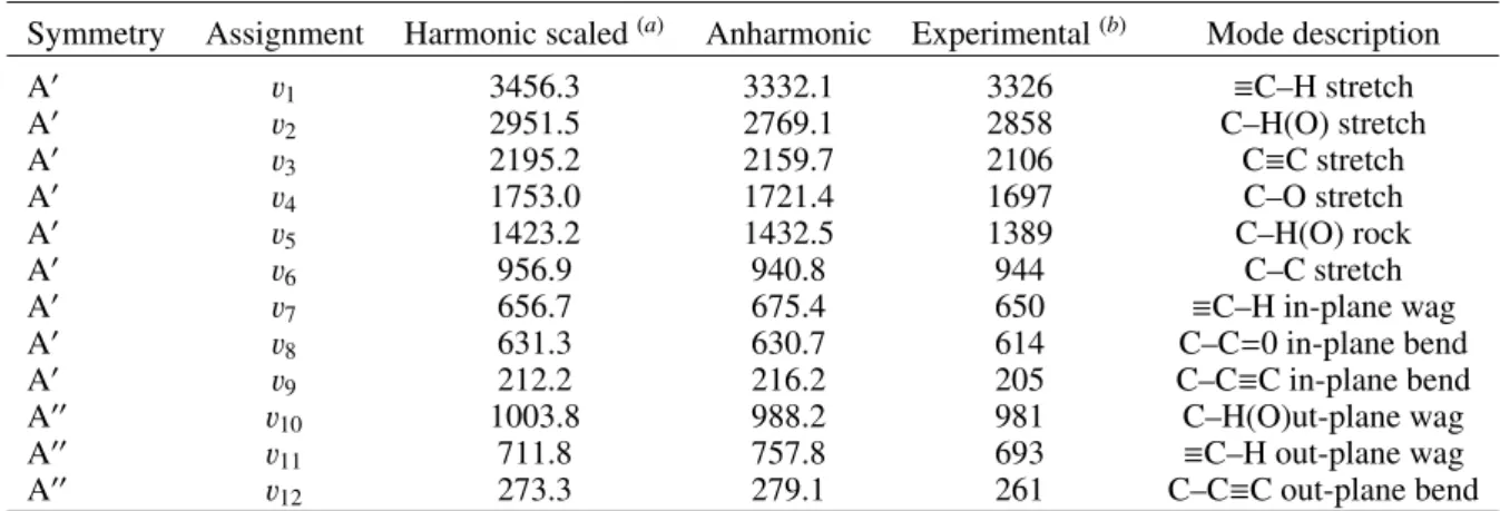
some of which have not yet been experimentally observed. As such, we carried out computational chemistry calculations at a B3LYP level of theory using a 6-311+G(d) basis set using the Gaussian16 (Frisch et al. 2016) to derive the complete set. Table 3 lists the fundamental vibrations of propynethial, their symmetry and mode description in addition to their predicted and experimental band centers. In order to determine the accu-racy of the predictions, additional calculations were also carried out on the oxygen analog, propynal, and the predictions were compared to the experimental values (see Table4). As can be seen from the calculations on propynal, the anharmonic calcula-tions are significantly different to those observed experimentally. The best methodology therefore is to scale the B3LYP funda-mental harmonic frequencies by using the appropriate scaling factor2 and not using the anharmonic values in estimating the band centers. This methodology was applied to the computa-tional chemistry calculations carried out on propynethial.
The tabulated values for the partition function are given in Table5, with Qtot(T ) = Qvib(T )Qrot(T ). We considered various
temperatures. Qrotis approximated as
Qrot= s Q ABC kT h !3 (1) The vibrational partition function was calculated with respect to the zero-point level using the following expression:
Q(T )vib= 3N−6 Y i=1 1 1 − e−Ei/kT. (2)
The experimental rotational constants in this calculation come from our analysis. The experimental vibrational states fre-quencies are those fromKargamanov et al.(1987) corrected for the matrix effect, except for the two lowest states not experimen-tally observed where we used the calculated scaled harmonic fre-quencies.
Table 1. Spectroscopic parameters of propynethial in MHz – S reduction.
Parameter This work(a) Brown et al.(b) Crabtree et al.(c)
A 42652.03185 (40)(d) 42652.0294 (43) 42647.85212 (85) B 3109.382386 (28) 3109.38236 (29) 3109.38225 (15) C 2894.265480 (28) 2894.26592 (40) 2894.26559 (20) DJ× 103 1.1298295 (90) 1.1282 (18) 1.1408 (18) DJK× 103 −104.85202 (18) −104.776 (65) −105.140 (58) DK× 103 4175.501 (13) 4168.8 (11) d1× 103 −0.2110838 (23) −0.20997 (62) −0.2110 (16) d2× 103 −0.00553372 (66) −0.00621 (60) HJ× 106 0.0025203 (11) HJK× 106 −0.150948 (27) HK J× 106 −21.5143 (21) −18.3 (30) HK× 106 1221.05 (19) h1× 109 0.864444 (40) h2× 109 0.04881 (19) h3× 109 0.014484 (16) LJ× 1012 −0.007289 (45) LJ JK× 1012 0.3320 (16) LJK× 1012 −6.50 (19) LKK J× 109 7.5537 (67) LK× 109 −464.2 (12) l1× 1015 −2.984 (21) l2× 1015 −0.189 (13) l4× 1015 −0.0579 (72) PK J× 1012 −0.01525 (42) PKK J× 1012 −2.1714 (65) PK× 1012 160.6 (25)
Number of distinct lines 3288 53 24
Standard deviation of the fit (in kHz) 26.7 8.9 1.4
FMax(in GHz) 630 40 52
JMax, Ka,Max 107, 24 20, 5 6, 1
Notes.(a)Watson’s S reduction was used in the representation Ir.(b)Brown et al.(1982).(c)Crabtree et al.(2016).(d)Numbers in parentheses are
one standard deviation in units of the least significant figures.
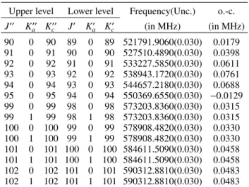
Table 2. Measured frequencies of propynethial and residuals from the fit.
Upper level Lower level Frequency(Unc.) o.-c.
J00 K00 a Kc00 J0 K0a K0c (in MHz) (in MHz) 90 0 90 89 0 89 521791.9060(0.030) 0.0179 91 0 91 90 0 90 527510.4890(0.030) 0.0398 92 0 92 91 0 91 533227.5850(0.030) 0.0611 93 0 93 92 0 92 538943.1720(0.030) 0.0761 94 0 94 93 0 93 544657.2180(0.030) 0.0688 95 0 95 94 0 94 550369.6550(0.030) −0.0129 99 0 99 98 0 98 573203.8360(0.030) 0.0315 99 1 99 98 1 98 573203.8360(0.030) 0.0315 100 0 100 99 0 99 578908.4820(0.030) 0.0330 100 1 100 99 1 99 578908.4820(0.030) 0.0330 101 0 101 100 0 100 584611.5090(0.030) 0.0458 101 1 101 100 1 100 584611.5090(0.030) 0.0458 102 0 102 101 0 101 590312.8810(0.030) 0.0483 102 1 102 101 1 101 590312.8810(0.030) 0.0483
Notes. Full fit is available at the CDS: S1.
The seven lowest vibrational excited state levels were con-sidered. The remaining ones above 900 cm−1 (1295 K) were found to have no influence on the partition function calculations.
5. Radioastronomical observations
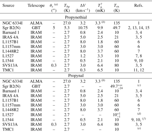
We searched for both propynethial and its oxygen-substituted counterpart propynal in a number of astronomically observed datasets, most of which are publicly available and all of which have previously been published elsewhere. These include ALMA observations of the high-mass star-forming region NGC 6334I (Brogan et al. 2018;McGuire et al. 2018a,2017), obser-vations of the Sgr B2N high-mass star-forming region using the Green Bank Telescope (GBT) from the Prebiotic Interstellar Molecule Survey (PRIMOS) project (Neill et al. 2012), as well as the datasets from the Astrochemical Surveys at IRAM (ASAI) Large Program, which was conducted with the IRAM 30 m tele-scope. The ASAI spectra cover a range of source types, from cold, dark clouds to class 0/1 protostars and shocked outflows, with observational details available inLefloch et al.(2018). We note that the frequency coverage of the ASAI observations varies from source to source (Fig. A.1). As a result, some favorable transitions of our target species are not covered.
The observational details of these sources are described else-where; here, we focus only on the salient physical parameters necessary to derive column densities. In the case of propynethial, because these are non-detections, we had to make assumptions about the physical conditions in which the molecules might be found. For sources with detections of propynal (Sgr B2N,
Table 3. Comparison of the band positions (cm−1) for propynethial from ab initio and density functional theory methods using a 6-311+G(d) basis
set.
Symmetry Assignment Harmonic Scaled(a) Experimental(b) Mode description
A0 v1 3458.6 3341.0 3315 ≡C–H stretch A0 v 2 3085.4 2980.5 – C–H (thial) stretch A0 v 3 2176.7 2102.7 2092 C≡C stretch A0 v4 1363.5 1317.1 1320 C–H (thial) rock A0 v 5 1128.1 1089.7 1107 C–S stretch A0 v6 911.9 880.9 895 C–C stretch A0 v 7 625.6 604.3 664 ≡C–H in-plane wag A0 v8 515.1 497.6 492 C–C–S in-plane bend A0 v 9 196.6 189.9 – C–C≡C in-plane bend
A00 v10 859.2 830.0 895 C–H (thial) out-plane wag
A00 v11 674.9 651.9 624 ≡C–H out-plane wag
A00 v
12 319.8 308.4 – C–C≡C out-plane bend
Notes.(a)B3LYP values scaled by 0.966.(b)Kargamanov et al.(1987).
Table 4. Comparison of the band positions (cm−1) for propynal from ab initio and density functional theory methods using a 6-311+G(d) basis set.
Symmetry Assignment Harmonic scaled(a) Anharmonic Experimental(b) Mode description
A0 v 1 3456.3 3332.1 3326 ≡C–H stretch A0 v2 2951.5 2769.1 2858 C–H(O) stretch A0 v 3 2195.2 2159.7 2106 C≡C stretch A0 v4 1753.0 1721.4 1697 C–O stretch A0 v 5 1423.2 1432.5 1389 C–H(O) rock A0 v6 956.9 940.8 944 C–C stretch A0 v7 656.7 675.4 650 ≡C–H in-plane wag A0 v 8 631.3 630.7 614 C–C=0 in-plane bend A0 v9 212.2 216.2 205 C–C≡C in-plane bend A00 v 10 1003.8 988.2 981 C–H(O)ut-plane wag A00 v11 711.8 757.8 693 ≡C–H out-plane wag A00 v 12 273.3 279.1 261 C–C≡C out-plane bend
Notes.(a)B3LYP values scaled by 0.966.(b)Brand et al.(1963).
TMC-1, and L1527), we used the physical parameters derived for that molecule to estimate the upper limits to the column den-sity and the abundance of propynethial in that source. For the other sources, we used the parameters from the literature. These parameters and the literature sources they were obtained from are provided in the respective tables.
5.1. Upper-limit analysis and results
We find no evidence of propynethial in any of our studied sources (Fig. 1). Propynal is known in TMC-1, Sgr B2(N), and Barnard 1 from prior work (Irvine et al. 1988;Turner 1991;
Loison et al. 2016), and we report a detection in L1527, which, to
the best of our knowledge, has not been previously seen in these data. All upper limits to propynethial and propynal are derived using the formalisms outlined inTurner(1991) that assume the molecules are well described by a single excitation tempera-ture and include corrections for optical depth. In this case, all transitions considered for both propynal and propynethial are extremely optically thin (τ 1) in all sources. Frequencies, energy levels, degeneracies, and line strengths were obtained from the laboratory spectroscopy described in this work. The partition function for each molecule, which includes a correc-tion for the lowest torsional vibracorrec-tional mode of the molecule, is given in Tables B.1 and6. Both species possess some low-lying vibrational modes that might contribute non-trivially to the
partition function. For propynal, the experimentally determined vibrational energies in Table4 were used; the scaled harmonic frequencies presented in Table3were used for propynethial.
For each source, we simulated a spectrum of each molecule using the physical conditions for the source (including any effects of beam dilution) and the line parameters measured in this work. Then, the 1σ upper limit to the column density was derived using the line that gave the most rigorous constraint (i.e., the line that would be the highest signal to noise in the event of a detection). These lines are provided in TablesB.1and6along with the resulting upper limits. We note that in some cases, mul-tiple transitions of a species contribute to single line due to close frequency spacings.
5.2. Propynal detections and comparison to propynethial 5.2.1. Sgr B2N
A detection of propynal in Sgr B2(N) was reported by Turner
(1991) in his 1989 survey data obtained with the NRAO 12-m telescope (the telescope diameter was actually 11 m for much of the work and was only resurfaced to 12 m for the final por-tions). From that study, we utilized the excitation temperature and linewidth of 49.7 K and 10.75 km s−1, respectively. To the best of our knowledge, the source was assumed to fill the beam,
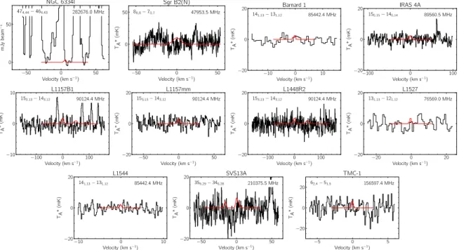
−50 0 50 Velocity (km s−1) 0 50 mJy beam − 1 474,44− 464,43 282676.0 MHz NGC 6334I −50 0 50 Velocity (km s−1) 0 50 TA * (mK) 80,8− 70,7 47953.5 MHz Sgr B2(N) −10 0 10 Velocity (km s−1) −20 0 20 TA * (mK) 141,13− 131,12 85442.4 MHz Barnard 1 −100 0 100 Velocity (km s−1) −20 0 20 TA * (mK) 150,15− 140,14 89560.5 MHz IRAS 4A −100 0 100 Velocity (km s−1) −10 0 10 TA * (mK) 153,13− 143,12 90124.4 MHz L1157B1 −50 0 50 Velocity (km s−1) −20 0 20 TA * (mK) 153,13− 143,12 90124.4 MHz L1157mm −100 0 100 Velocity (km s−1) −20 0 20 TA * (mK) 153,13− 143,12 90124.4 MHz L1448R2 −20 0 20 Velocity (km s−1) −20 0 20 TA * (mK) 131,13− 121,12 76569.0 MHz L1527 −10 0 10 Velocity (km s−1) −20 0 20 TA * (mK) 141,13− 131,12 85442.4 MHz L1544 −50 0 50 Velocity (km s−1) −20 0 20 TA * (mK) 356,29− 346,28 210375.5 MHz SVS13A −5 0 5 Velocity (km s−1) −20 0 20 TA * (mK) 62,4− 51,5 156597.4 MHz TMC-1
Fig. 1.Transitions of propynethial used to calculate the upper limits given in Table6. In each panel, the red trace shows the transition simulated using the derived upper-limit column density and the physical parameters assumed for that source. The frequency of the transition is given in the top right of each panel, and the quantum numbers for each transition in the top left. The source name is given above each panel. Due to the large variances between observations, the intensity and velocity axes are not uniform between each panel.
Table 5. Rotational, vibrational, and total partition functions at various temperatures.
T(K) Q(T )rot Q(T )vib Q(T )tot
300 45081.1967 2.6993 121691.2866 225 29244.4671 1.7955 52508.8426 150 15886.3223 1.2752 20257.9079 75 5605.5584 1.0297 5771.8927 37.5 1980.7762 1.0007 1982.1418 18.75 700.7635 1.0000 700.7635 9.375 248.2981 1.0000 248.2981
which varied from 60–8000 between the highest and lowest-frequency transitions observed (83.8 and 113.8 GHz).
As far as we know, the data from theTurner(1989) survey is not currently available in electronic format, precluding a detailed analysis. A cursory look at the spectra presented in that survey via the article figures showed no indication of any transitions of propynethial above the reported noise limits in any passband.
We were able to perform a more complete search in this source using the data available from the GBT PRIMOS program. The most prominent transitions predicted in these data were between 45 and 50 GHz. The GBT beam at 48 GHz where the upper limit was derived is 1600. If both propynethial and
propy-nal did indeed fill the larger 12-m beam, then there would be no mismatch from the observations, and we would derive an abun-dance ratio of [propynethial]/[propynal] of <1.5.
However,Hollis et al. (2007) derived a 500 source size for warm, compact emission from complex molecules. This more compact size for warmer molecular emission has been seen in numerous other studies in the recent literature (see, e.g.,
Belloche et al. 2014 and Bonfand et al. 2017). If we adopted
this source size instead, we would derive an upper limit of propy-nethial of <6.7×1014cm−2from the PRIMOS observations. If we adopted an average 7000beam size for theTurner(1991)
analy-sis, the column density of propynal would increase to 7.3 × 10¹⁵,
resulting in a [propynethial]/[propynal] ratio of <0.1. 5.2.2. L1527
The ASAI data toward L1527 contain several spectral lines of propynal with a sufficiently high S/N to derive a column density and excitation temperature. The resolution of the ASAI obser-vations (195 kHz; 0.3–0.8 km s−1) do not provide sufficient
res-olution elements across these weak lines (∆V = 1.2 km s−1).
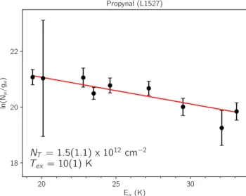
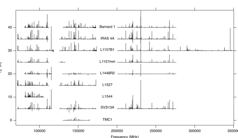
As a result, the parameters derived from Gaussian fits to these lines have large statistical uncertainties (Table B.2). We used these values and the associated uncertainties to construct a rota-tion diagram (Goldsmith & Langer 1999) of propynal in L1527 and derive a column density and excitation temperature, assum-ing the source fills the beam (Fig.2). The spectrum of propy-nal simulated using our derived best fit parameters is shown in Fig.B.1 compared to the observational data for all transitions with S/N >3. These are the same transitions used to generate the rotation diagram. To our knowledge, propynal has not pre-viously been reported in this source. Combined with our propy-nethial upper limit (derived using the values of Tex and ∆V
determined for propynal), we derive an abundance ratio of [propynethial]/[propynal] of <7.
5.2.3. TMC-1
The first reported detection of propynal in the ISM was byIrvine
et al.(1988) in the Nobeyama 45-m observations of TMC-1. The
beam size of the Nobeyama 45 m varied from 90 to 4500between
the two measured transitions at 18.7 and 37.3 GHz, respectively. The IRAM 30-m beam is 1600 at 156.6 GHz, where the propy-nethial upper limit was derived. Especially for small molecules, the size of the emitting region is assumed to be much larger than any of these (Kaifu et al. 2004), thus we assume the beam size mismatch is not likely to be an issue in the comparison. We used the Tex from that work of 10 K to derive the upper
20 25 30 Eu(K) 18 20 22 ln(N u /g u ) Propynal (L1527) NT = 1.5(1.1) x 1012 cm−2 Tex = 10(1) K
Fig. 2. Rotation diagram of propynal detection in L1527, using the lines and parameters reported in TableB.2. The reported errors in col-umn density and temperature are the 1σ statistical errors from the least squares fit to the data, while the error bars for the data points are derived from the 1σ statistical errors in intensity and velocity width from the Gaussian fits to the lines.
limit to propynethial in our work. The resulting abundance ratio of [propynethial]/[propynal] is <1.7 in TMC-1. We note that
Loison et al. (2016) also reported a detection of propynal in
TMC-1. Their reported column density of 8.0 × 1011cm−2falls
slightly outside the uncertainty of the measurement of Irvine
et al. (1988). However, because Loison et al. (2016) do not
appear to have provided an uncertainty on their measurement, we cannot comment more on any potential disagreement between the values.
5.2.4. L1544
Jimenez-Serra et al. (2016) reported a single-line (90,9−80,8)
detection of propynal in L1544 using the IRAM 30-m telescope, deriving a column density of 1.8−6.3 × 1011cm−2over a range of assumed Tex = 5−10 K toward the dust-continuum peak in
L1544 (corresponding to the same pointing location as the ASAI data). While Fig. 1 ofJimenez-Serra et al.(2016) does appear to show a reasonable S/N corresponding to the 90,9−80,8, we do not
see any emission in the ASAI data at this frequency. Our derived upper limit of 6.4 × 1010cm−2 is outside the range of column
densities derived byJimenez-Serra et al. (2016) if we assume Tex= 10 K, as we do here. If we were instead to assume Tex= 5 K
and use the 90,9−80,8transition as our fiducial, we would derive a
column density of 2.9 × 1011 cm−2, in agreement with
Jimenez-Serra et al.(2016). Figure3shows simulations of the 90,9−80,8
from our derived upper limits compared to the observations, with a shaded curve representing the range of line profiles that would result from the values derived in Jimenez-Serra et al.(2016). Based on the ASAI observations, and the lack of emission in any other transition of propynal covered by these observations, we conclude that the ASAI data do not support a detection of propynal in L1544, and set an upper limit of 6.4 × 1010cm−2 based on these results.
5.3. Barnard 1
Loison et al. (2016) report a single-line (90,9−80,8) detection
of propynal in Barnard 1, deriving a column density of 7.9 × 1011cm−2. This is ∼5× higher than our 1σ upper limit. Indeed,
−10
0
10
Velocity (km s
−1)
0
20
T
A
*
(mK)
9
0,9− 8
0,883775.8 MHz
L1544
Fig. 3.Simulation of the 90,9−80,8transition of propynal toward L1544
using our derived upper-limit parameters in red over the ASAI observa-tions in black. The shaded blue curve represents the range of potential line profiles for this transition based on the values reported in Jimenez-Serra et al.(2016).
the 90,9−80,8transition of propynal is covered by the ASAI data,
and no emission is seen. We attempted to reconcile the differ-ences, before making a comparison to propynethial. The salient parameters are presented in Table7.
For comparison, we simulated the spectra of propynal using the 0.6 km s−1 linewidth from Loison et al. (2016) using both
their derived column density and our upper limit. We used our value for the partition function (Q[10 K]= 142) for both simula-tions. The resulting spectra for the 90,9−80,8observed inLoison
et al.(2016) as well as the 110,11−100,10 transitions we used to
set our upper limit are shown in Fig.4. While theLoison et al.
(2016) column density is consistent within the ∼3σ noise level of the ASAI observations for the 90,9−80,8, it overproduces the
observations for the 110,11−100,10 transition we use to set our
upper limit. Further complicating matters,Loison et al.(2016) do not appear to have provided an estimate of the uncertainty in their derived column density.
Nevertheless, visually, the detection of the 90,9−80,8
pre-sented in Fig. 1 ofLoison et al.(2016) appears significant. Thus, while the ASAI observations cannot confirm that detection, and there are discrepancies we are unable to resolve, we feel it is worthwhile to report a ratio to our propynethial upper limit here. Depending on whether a linewidth of 0.6 or 0.8 km s−1is used, our derived upper limit varies between 5.8–9.1 × 1011cm−2for
propynethial. Taking the propynal column of 7.9 × 1011cm−2
from Loison et al. (2016), the resulting abundance ratio of
[propynethial]/[propynal] is <0.7−1.5 in Barnard 1.
6. Discussion
The measurements of the submillimeter-wave spectrum of propy-nethial reported here have allowed accurate predictions of line positions and intensities through ∼700 GHz. These new mea-surements have enabled us to search for this species in a num-ber of datasets at millimeter and submillimeter wavelengths, and set upper limits to the abundance of propynethial with con-fidence. The non-detection of propynethial in the 11 different astronomical sources searched here adds to a growing list of sulfur analogs to known interstellar species that have not yet
Table 6. Upper limits to propynethial and the line parameters used to calculate them in each of the sets of observations.
Source Frequency Transition Eu Si jµ2 Q(Qrot, Qvib) (a) NT N(H2) XH2 Refs. (MHz) (J0 Ka,Kc− J 00 Ka,Kc) (K) (Debye 2) (cm−2) (cm−2) N(H 2) NGC 6334I 282676.0 474,44−464,43 478.7 140.7 16358 (13560, 1.21) ≤1.5 × 10¹⁶ – – – Sgr B2(N) 47956.5 80,8−70,7 10.4 24.9 3032 (3019, 1.00) ≤6.2 × 10¹³ 1 × 1024 ≤6 × 10⁻¹¹ 1 Barnard 1 85442.4 141,13−131,12 32.7 43.3 275 (275, 1.00) ≤9.1 × 10¹¹ 1.5 × 10²³ ≤6 × 10⁻¹² 3 IRAS 4A 89560.5 150,15−140,14 34.5 46.6 830 (830, 1.00) ≤2.3 × 10¹² 3.7 × 10²³ ≤6 × 10⁻¹² 3 L1157B1 90124.4 153,13−143,12 51.7 44.8 4051 (4006, 1.01) ≤2.3 × 10¹² 1 × 10²¹ ≤2 × 10⁻⁹ 3 L1157mm 90124.4 153,13−143,12 51.7 44.8 4051 (4006, 1.01) ≤1.5 × 10¹² 6 × 10²¹ ≤3 × 10⁻¹⁰ 3 L1448R2 90124.4 153,13−143,12 51.7 44.8 4051 (4006, 1.01) ≤4.7 × 10¹² 3.5 × 10²³ ≤1 × 10⁻¹¹ 4 L1527 76569.0 131,13−121,12 27.7 40.2 275 (275, 1.00) ≤1.1 × 10¹² 2.8 × 10²² ≤4 × 10⁻¹¹ 4 L1544 85442.4 141,13−131,12 32.7 43.3 275 (275, 1.00) ≤4.0 × 10¹¹ 5 × 10²¹ ≤8 × 10⁻¹¹ 5 SVS13A 210375.5 353,33−343,32 198.8 108.0 6409 (6174, 1.04) ≤1.1 × 10¹⁶ 3 × 1024 ≤4 × 10⁻⁹ 6 TMC1 156597.4 62,4−51,5 13.7 1.0 275 (275, 1.00) ≤2.6 × 10¹² 1 × 10²² ≤3 × 10⁻¹⁰ 3
Notes.(a)Calculated at the excitation temperature assumed for the source. See TableA.1.
References. [1]Lis & Goldsmith(1990), [2]Crockett et al.(2014), [3]Cernicharo et al.(2018), [4]Jørgensen et al.(2002), [5]Vastel et al.(2014), [6]Chen et al.(2009).
Fig. 4. Simulations of propynal emission in the 90,9−80,8 and
110,11−100,10transitions overlaid on the ASAI observations of Barnard
1. The bold, blue trace represents the expected emission profile given the column density and linewidth reported in Loison et al. (2016), although using our partition function. The thinner red trace is the upper limit presented from our work, simulated using the linewidth from
Loison et al.(2016).
been found in the ISM. Recent examples include thioacetaldehyde
(CH3CHS;Margulès et al. 2020), thioketene (H2CCS;McGuire
et al. 2019), ethynethiol (HCCSH; McGuire et al. 2019), and
thioacetamide (CH3C(S)NH2; Remijan et al., in prep.).
The [propynethial]/[propynal] abundance ratios reported here are relatively large (<0.1–17) compared to the solar sulfur-to-oxygen ratio of ∼0.02 (Cameron 1973). The largest factor contributing to the non-detection is certainly the abundance of propynethial and the associated formation and destruction chemistry. A detailed analysis of the molecular reaction network and modeling is beyond the scope of this work, but would be a useful related study.
Aside from abundance, there are two major factors that contribute to the difficulty of detecting propynethial relative to propynal: its partition function (Q) and permanent dipole moment components (µa and µb). Assuming the transitions are
described by a single excitation temperature in the optically thin limit, the intensity of an observed transition (I) is proportional to the square of the dipole moment and the inverse of the partition function (cf., Eq. (1) ofHollis et al. 2004):
I ∝ µ
2
Q. (3)
Carvajal et al.(2019) recently reviewed the importance and
impact of partition functions in the derivation of abundances of
Table 7. Comparison of observational and source parameters for Barnard 1 in this work and in that ofLoison et al.(2016).
Parameter Loison et al.(2016) This work RA (J2000) 30h33m20s.8 30h33m20s.8 Dec (J2000) 31◦0703400 31◦0703400
Spec. resolution (kHz) 50(a) 195
RMS at 84 GHz (mK) 4–6 6.5
Linewidth (km s−1) 0.6 0.8
Tex(K) 10 10
Q(10 K) Not provided 142
Notes.(a)Cernicharo et al.(2012).
interstellar molecules. In this case, the vibrational contributions to both species are quite similar. However, the increased mass of sulfur in propynethial results in rotational constants ∼33% smaller than propynal. As shown in Eq. (1), this has the effect
of increasing the rotational contribution to the partition function for propynethial by a factor of
√
0.63−3≈ 2. This in turn reduces
the intensity of propynethial transitions relative to propynal by the same amount (cf., Eq. (3)).
The dipole moment components of propynal were reported
in Brown et al. (1982) to be µa = 2.4 and µb = 1.468. The
components for propynethial are smaller by factors of 0.75 and 0.45, respectively. Because the strength of the transitions relies on µ2, propynethial transitions are weaker than the
correspond-ing propynal transitions by factors of ∼1.8 and ∼4.9 for a- and b-type transitions.
These two factors combine to make propynethial ∼3.6–9.8 times more difficult to detect than propynal, explaining the comparatively high relative abundance limits that we were able to set here. Given that the most rigorous constraints were those set in Sgr B2(N) and Barnard 1 of 0.1–1.5, depending on source size assumptions, these sources are likely the best to conduct follow-up targeted searches for propynethial. Using the source and molecule parameters assumed here, the best limits might be set by observations with the Next Generation Very Large Array (ngVLA;Selina et al. 2018) near ∼80 GHz.
7. Conclusions
We recorded the submillimeter-wave spectrum of propynethial up to 630 GHz. In total, 3288 new transitions were measured and assigned to the ground state, which permits accurate predictions up to 700 GHz. The four lowest vibrational states, ν5=1, ν9=1,
ν12=1, ν9=2, and ν8=1, are all strong enough in our spectrum
to be assigned, and an analysis of these states together with the ground state is in progress. A search for propynethial and propy-nal was conducted in a number of astrophysical environments. Propynethial was not detected in any source, and upper limits were derived. Propynal was detected for the first time in L1527.
Acknowledgements. The present investigations were supported by the CNES
and the CNRS program “Physique et Chimie du Milieu Interstellaire” (PCMI). J. C. G. thanks the Centre National d’Etudes Spatiales (CNES) for a grant. Sup-port for B. A. M. was provided by NASA through Hubble Fellowship grant #HST-HF2-51396 awarded by the Space Telescope Science Institute, which is operated by the Association of Universities for Research in Astronomy, Inc., for NASA, under contract NAS5-26555. The National Radio Astronomy Observatory is a facility of the National Science Foundation operated under cooperative agreement by Associated Universities, Inc.
References
Araki, M., Takano, S., Sakai, N., et al. 2017,ApJ, 847, 51
Barros, J., Appadoo, D., McNaughton, D., et al. 2015,J. Mol. Spectr., 307,
44
Belloche, A., Garrod, R. T., Müller, H. S. P., & Menten, K. M. 2014,Science,
345, 1584
Bonfand, M., Belloche, A., Menten, K. M., Garrod, R. T., & Müller, H. S. P.
2017,A&A, 604, A60
Brand, J., Callomon, J., & Watson, J. 1963,Discuss. Faraday Soc., 35, 175
Brogan, C. L., Hunter, T. R., Cyganowski, C. J., et al. 2018,ApJ, 866, 87
Brown, R. D., Godfrey, P. D., Champion, R., & Woodruff, M. 1982,Aust. J.
Chem., 35, 1747
Cameron, A. G. W. 1973,Space Sci. Rev., 15, 121
Carvajal, M., Favre, C., Kleiner, I., et al. 2019,A&A, 627, A65
Cernicharo, J., Marcelino, N., Roueff, E., et al. 2012,ApJ, 759, L43
Cernicharo, J., Lefloch, B., Agúndez, M., et al. 2018,ApJ, 853, L22
Chen, X., Launhardt, R., & Henning, T. 2009,ApJ, 691, 1729
Costain, C. C., & Morton, J. R. 1959,J. Chem. Phys., 31, 389
Crabtree, K. N., Martin-Drumel, M.-A., Brown, G. G., et al. 2016,J. Chem.
Phys., 144, 124201
Crapsi, A., Caselli, P., Walmsley, C. M., et al. 2005,ApJ, 619, 379
Crockett, N. R., Bergin, E. A., Neill, J. L., et al. 2014,ApJ, 787, 112
Frisch, M., Trucks, G., Schlegel, H., et al. 2016,Gaussian 16(Wallingford, CT:
Gaussian, Inc.)
Gal, Y.-S., & Choi, S.-K. 1988,J. Polym. Sci. Part C: Polym. Lett., 26, 115
Goldsmith, P. F., & Langer, W. D. 1999,ApJ, 517, 209
Gratier, P., Majumdar, L., Ohishi, M., et al. 2016,ApJS, 225, 1
Higuchi, A. E., Sakai, N., Watanabe, Y., et al. 2018,ApJS, 236
Hily-Blant, P., Faure, A., Vastel, C., et al. 2018,MNRAS, 480, 1174
Hollis, J. M., Jewell, P. R., Lovas, F. J., & Remijan, A. 2004,ApJ, 613, L45
Hollis, J. M., Jewell, P. R., Remijan, A. J., & Lovas, F. J. 2007,ApJ, 660,
L125
Howe, J. A., & Goldstein, J. H. 1955,J. Chem. Phys., 23, 1223
Irvine, W. M., Brown, R., Cragg, D., et al. 1988,ApJ, 335, L89
Jimenez-Serra, I., Vasyunin, A. I., Caselli, P., et al. 2016,ApJ, 830, 1
Jørgensen, J. K., Schöier, F. L., & van Dishoeck, E. F. 2002,A&A, 389, 908
Kaifu, N., Ohishi, M., Kawaguchi, K., et al. 2004,PASJ, 56, 69
Kargamanov, N. D., Korolev, V. A., & Mal’tsev, A. K. 1987,Russian. Chem.
Bull., 36, 2152
Kisiel, Z. 2001,Spectroscopy from Space(Springer), 91
Laas, J. C., & Caselli, P. 2019,A&A, 624, A108
Lefloch, B., Bachiller, R., Ceccarelli, C., et al. 2018,MNRAS, 477, 4792
Lis, D. C., & Goldsmith, P. F. 1990,ApJ, 356, 195
Loison, J.-C., Agúndez, M., Marcelino, N., et al. 2016,MNRAS, 456, 4101
Margulès, L., Ilyushin, V.V., McGuire, B.A., et al. 2020,J. Mol. Spectr., 371,
111304
Martín-Doménech, R., Jiménez-Serra, I., Caro, G. M., et al. 2016,A&A, 585,
A112
McGuire, B. A. 2018,ApJS, 239, 17
McGuire, B. A., Carroll, P. B., Dollhopf, N. M., et al. 2015,ApJ, 812, 1
McGuire, B. A., Carroll, P. B., Loomis, R. A., et al. 2016,Science, 352, 1449
McGuire, B. A., Shingledecker, C. N., Willis, E. R., et al. 2017,ApJ, 851, L46
McGuire, B. A., Brogan, C. L., Hunter, T. R., et al. 2018a,ApJ, 863, L35
McGuire, B. A., Burkhardt, A. M., Kalenskii, S. V., et al. 2018b,Science, 359,
202
McGuire, B. A., Shingledecker, C. N., Willis, E. R., et al. 2019,ApJ, 883, 201
Melosso, M., Melli, A., Puzzarini, C., et al. 2018,A&A, 609, A121
Nefedov, O. M., Korolev, V. A., Zanathy, L., Soloukie, B., & Bock, H. 1992,
Mendeleev Commun., 2, 67
Neill, J. L., Muckle, M. T., Zaleski, D. P., et al. 2012,ApJ, 755, 153
Pickett, H. M. 1991,J. Mol. Spectr., 148, 371
Remijan, A. J., Hollis, J. M., Lovas, F. J., et al. 2008,ApJ, 675, L85
Selina, R. J., Murphy, E. J., McKinnon, M., et al. 2018, ed. E. Murphy, Science with a Next Generation Very Large Array, 15
Turner, B. E. 1989,ApJS, 70, 539
Turner, B. E. 1991,ApJS, 76, 617
Vastel, C., Ceccarelli, C., Lefloch, B., & Bachiller, R. 2014,ApJ, 795, L2
Widicus Weaver, S., Butler, R., Drouin, B., et al. 2005,ApJS, 158, 188
Winnewisser, G. 1973,J. Mol. Spectr., 46, 16
Wong, A. 2016, PhD Thesis, Monash University, Australia
Zakharenko, O., Motiyenko, R. A., Margulès, L., & Huet, T. R. 2015,J. Mol.
Appendix A: Observational source parameters
Table A.1. Source parameters assumed for propynethial in each of the sets of observations, and for propynal in those observations that resulted in a non-detection.
Source Telescope θs(a) Tbg ∆V Tb† Tex Refs.
(00) (K) (km s−1) (mK) (K) Propynethial NGC 6334I ALMA – 27.0 3.2 3.3(b) 135 1 Sgr B2(N) GBT 5 5.3 10.75 9.9 49.7 2, 13, 14, 15 Barnard 1 IRAM – 2.7 0.8 2.4 10 3, 4 IRAS 4A IRAM – 2.7 5.0 2.5 21 3, 5 L1157B1 IRAM – 2.7 8.0 1.8 60 6 L1157mm IRAM – 2.7 3.0 3.0 60 6 L1448R2 IRAM – 2.7 8.0 3.7 60 7 L1527 IRAM – 2.7 1.2 3.3 10 7, 8 L1544 IRAM – 2.7 0.5 2.1 10 9, 10 SVS13A IRAM 0.3 2.7 3.0 6.4 80 3, 5 TMC1 IRAM – 2.7 0.3 6.5 10 11, 12 Propynal NGC 6334I ALMA – 27.0 3.2 3.3(b) 135 1 Sgr B2(N) GBT – 2.7 – – 49.7+∞−24 (c) Barnard 1 IRAM – 2.7 0.8 2.4 10 3, 4 IRAS 4A IRAM – 2.7 5.0 2.5 21 3, 5 L1157B1 IRAM – 2.7 8.0 1.8 60 6 L1157mm IRAM – 2.7 3.0 3.0 60 6 L1448R2 IRAM – 2.7 8.0 3.7 60 7 L1527 IRAM – 2.7 – – 10+1−1 (d) L1544 IRAM – 2.7 0.5 2.1 10 9, 10,( f ) SVS13A IRAM 0.3 2.7 3.0 6.4 80 3, 5 TMC1 IRAM – 2.7 – – 10 (e)
Notes.(a)Except where noted, the source is assumed to fill the beam.(b)For these interferometric observations, the intensity is given in mJy beam−1
rather than mK.(c)This detection was reported byTurner(1991). Individual fits to∆V and T†
b for this multiline detection are detailed inTurner
(1991); only the derived Texis reported here.(d)This detection is reported in this work. Individual fits to∆V and T †
b for this multiline detection
are detailed in TableB.2; only the derived Tex is reported here.(e)This detection was reported byIrvine et al.(1988). Individual fits to∆V and
Tb†for this multiline detection are detailed inIrvine et al.(1988); only the assumed Texis reported here.( f )Jimenez-Serra et al.(2016) reported a
single line (90,9−80,8) detection of propynal in L1544. See text and TableB.1for further discussion.†Taken either as the 1σ RMS noise level at the
location of the target line, or for line confusion limited spectra, the reported RMS noise of the observations.
References.Araki et al.(2017),McGuire et al.(2018a); [2]Neill et al.(2012); [3]Melosso et al.(2018); [4]Cernicharo et al.(2018); [5]Higuchi et al.(2018); [6]McGuire et al.(2015); [7]Jørgensen et al.(2002); [8]Araki et al.(2017); [9]Hily-Blant et al.(2018); [10]Crapsi et al.(2005); [11]McGuire et al.(2018b); [12]Gratier et al.(2016); [13]Remijan et al.(2008); [14]McGuire et al.(2016); [15]Turner(1991).
40 30 20 10 0 TA * (K) 350000 300000 250000 200000 150000 100000 Frequency (MHz) TMC1 SVS13A L1544 L1527 L1448R2 L1157mm L1157B1 IRAS 4A Barnard 1
Fig. A.1.Global overview of the frequency coverage of the ASAI data toward each source.
Appendix B: Propynal analysis
Table B.1. Propynal column densities and upper limits, with associated line parameters.
Source Frequency Transition Eu Si jµ2 Q(Qrot, Qvib)(a) NT N(H2) XH2 Refs. (MHz) (J0 Ka,Kc−J 00 Ka,Kc) (K) (Debye 2) (cm−2) (cm−2) N(H 2) NGC 6334I 280106.3 304,26−294,25 256.9 164.1 8323 (6908, 1.20) ≤3.6 × 10¹⁵ – – –
Sgr B2(N) Detection specifics reported inTurner(1991) 3.7+3.4−1.4× 10¹³ 1 × 1024 4 × 10⁻¹¹ 1 Barnard 1(c) 102298.1 11 0,11−100,10 29.5 61.2 142 (142, 1.00) ≤1.5 × 10¹¹ 1.5 × 10²³ ≤1 × 10⁻¹² 3 IRAS 4A 100716.9 111,11−101,10 32.1 60.7 424 (424, 1.00) ≤5.6 × 10¹² 3.7 × 10²³ ≤2 × 10⁻¹¹ 3 L1157B1 85361.2 91,8−81,7 23.5 49.5 2060 (2041, 1.01) ≤1.1 × 10¹¹ 1 × 10²¹ ≤1 × 10⁻¹⁰ 3 L1157mm 104302.2 111,10−101,9 33.1 60.7 2060 (2041, 1.01) ≤7.0 × 10¹¹ 6 × 10²¹ ≤1 × 10⁻¹⁰ 3 L1448R2 102298.1 110,11−100,10 29.5 61.2 2060 (2041, 1.01) ≤1.9 × 10¹² 3.5 × 10²³ ≤5 × 10⁻¹² 4
L1527 Detected in this work; see text and TableB.2 142 (142, 1.00) 1.5+1.0−1.0× 10¹¹ 2.8 × 10²² 5 × 10⁻¹² 4
L1544 93043.3 100,10−90,9 24.6 55.7 142 (142, 1.00) ≤6.4 × 10¹⁰ 5 × 10²¹ ≤1 × 10⁻¹¹ 5(b)
SVS13A 257153.6 280,28−270,27 180.2 155.8 3255 (3144, 1.04) ≤2.5 × 10¹⁵ 3 × 1024 ≤8 × 10⁻¹⁰ 6
TMC1 Detection specifics reported inIrvine et al.(1988) 1.5+0.4−0.4× 10¹² 1 × 10²² 2 × 10⁻¹⁰ 3
Notes.(a)Calculated at the excitation temperature assumed for the source. See TableA.1.(b)Jimenez-Serra et al.(2016) reported a column density
of (1.8−6.3) × 1011cm−2based on a single transition.(c)Loison et al.(2016) reported a detection of propynal in Barnard 1 that is not seen in the
ASAI observations with a column density of NT= 7.9 × 1011cm−2. See text for details.
References.Araki et al.(2017),Lis & Goldsmith(1990); [2]Crockett et al.(2014); [3]Cernicharo et al.(2018); [4]Jørgensen et al.(2002); [5]
Table B.2. Frequencies, quantum numbers, fit brightness temperatures and linewidths, and transition properties for lines used to derive the column density and excitation temperature of propynal in L1527.
Frequency(†) Transition T(‡) b ∆V (‡) E u Si jµ2 (MHz) (JK0 a,Kc−J 00 Ka,Kc) (mK) (km s −1) (K) (Debye2) 75885.2058 81,7−71,6 19.7(36) 1.4(2) 19.4 43.9 82424.9250 91,9−81,8 19.5(43) 1.6(4) 22.8 49.5 83775.8251 90,9−80,8 45.2(735) 0.7(9) 20.1 50.1 85361.1884 91,8−81,7 17.2(24) 1.1(1) 23.5 49.5 91572.5215 101,10−91,9 18.1(29) 1.5(2) 27.2 55.1 93043.2911 100,10−90,9 18.6(32) 1.7(3) 24.6 55.7 100716.8520 111,11−101,10 10.6(41) 0.8(3) 32.1 60.7 102298.0618 110,11−100,10 18.5(35) 0.9(2) 29.5 61.2 104302.2378 111,10−101,9 11.4(23) 1.3(3) 33.1 60.7
Notes.(†)Held fixed in the Gaussian fit to the catalog value. See text for estimates of uncertainties resulting from laboratory measurements.(‡)1σ
statistical uncertainty from the Gaussian fits to the data, in units of the last significant digit.
0 25 50 TA * (mK) 81,7− 71,6 75885.2 MHz 91,9− 81,8 82424.9 MHz 90,9− 80,8 83775.8 MHz 0 20 40 TA * (mK) 91,8− 81,7 85361.2 MHz 101,10− 91,9 91572.5 MHz 100,10− 90,9 93043.3 MHz −20 0 20 Velocity (km s−1) 0 20 TA * (mK) 111,11− 101,10 100716.9 MHz −20 0 20 Velocity (km s−1) 110,11− 100,10 102298.1 MHz −20 0 20 Velocity (km s−1) 111,10− 101,9 104302.2 MHz
Fig. B.1.Transitions of propynal identified in the ASAI data toward L1527 with an S/N ratio of ≥3. Transition parameters are given in TableB.2. The observational data are shown in black. A simulation of propynal using the derived best fit column density and temperature is shown in red using a noise-weighted average linewidth derived from our Gaussian fits to the individual lines (1.2 km s−1) and simulated at the same resolution