Adaptive Systems in Digital Communication Designs
by
Xinben Garrison Qian
Submitted to the Department of Electrical Engineering and Computer Science in partial fulfillment of the requirements for the degrees of
Bachelor of Science in Electrical Engineering and Computer Science and
Master of Science in Electrical Engineering and Computer Science at the
MASSACHUSETTS INSTITUTE OF TECHNOLOGY May 1996
© 1996 Xinben Garrison Qian All rights Reserved
The author hereby grants to MIT permission to reproduce and to distribute publicly paper and electronic copies of this thesis document in whole or in part.
Author Department of Electrical Engineering and Computer Science
Certified by Professor Richard D. Thornton Thesis Supervisor
/'"•/
Certified by Dr. Ganesh Rajan AA Tektronix SupervisorA-
A'
I
IM•
9
,
or.
a- -• F. R. MorgtthalerCha an, Depa 1 Committee on Graduate Students
OF TECHNOLO9Y
JUL
1
6
1996
LIBqAARiE Accepted by
Adaptive Systems in Digital Communication Designs
by
Xinben Garrison Qian
Submitted to the Department of Electrical Engineering and Computer Science on May
10, 1996, in partial fulfillment of the requirements for the degrees of Bachelor of Science
in Electrical Engineering and Computer Science and Master of Science in Electrical
Engineering and Computer Science.
Abstract
The desirable features of an adaptive system, namely, the ability to operate satisfactorily
in an unknown environment and also track time variations of input statistics, have make
it a powerful device to provide the robustness that is desired for all digital
communi-cation systems. An adaptive filter and a closed tracking loop are forms of an general
adaptive system. Applications of both forms are considered in this thesis. As an
adaptive filtering application, a linear adaptive transversal filter can be used to remove
undesirable distortion caused by an analog front end that is present in most digital
communication systems. As an closed tracking loop application, a delay-locked loop
(DLL) can be used to perform pseudo-noise (PN) code tracking, an essential task in
direct-sequence spread-spectrum communication systems.
Thesis Supervisor: Richard D. Thornton
Title: Professor of Electrical Engineering
Thesis Supervisor: Ganesh Rajan
Acknowledgments
I would like to first thank Ganesh Rajan for his encouragement and support without which this thesis would not be possible. And also I thank my good friend James Yang and Scott Velazquez for their great effort in proofreading this paper. James, Scott, beers will be on me next time. Of course, I have not forgot my fellow co-opers at Tektronix, Kathy Chiu and Johnson Tan. With you guys around, life, no matter how unfair sometimes, will always be fun. At last I would like to thank my dear aunt Binky, and my parents for the love they have given me through the years. I love you all.
Contents
ACKNOWLEDGMENTS ... 3
CHAPTER 1 : INTRODUCTION ... 10
1.1 RECEIVER FRONT END CORRECTION PROBLEM ... ... 11
1.2 CODE TRACKING IN DIRECT-SEQUENCE SPREAD-SPECTRUM SYSTEMS ... 12
1.3 O RG AN IZATIO N ... ... 13
CHAPTER 2: FRONT END CORRECTION PROBLEM ... 14
2.1 FRONT END DISTORTION STUDY ... ... 15
2.1.1 G SM Sim ulation ... ... 20
2.1.2 C D M A Sim ulation ... .. ... ... 31
2.2 ADAPTIVE FRONT END EQUALIZATION ... 38
2.2.1 A dap tive F ilters... ... 39
2.2.2 Front End E qualization... ... 47
2.3 C ONCLUSIONS ... . ... 57
CHAPTER 3: CODE SYNCHRONIZATION USING DELAY-LOCKED LOOPS...58
3.1 SPREAD-SPECTRUM COMMUNICATION SYSTEM... .. ... 58
3.1.1 Pseudo-Noise (PN) Sequence... ... .. . ... 60
3.1.2 Direct-Sequence Spread-Spectrum System ... 62
3.1.3 C ode Synchronization ... 65
3.2 ANALYSIS AND SIMULATIONS OF NON-COHERENT DLLS... ... 68
3.2.1 Non-Coherent Delay-Locked Loop... 68
3.2.2 D LL Sim ulation ... ... 79
3.2.3 Linear First-Order DLL For Optimum Tracking Performnance... 84
CH APTER 4 : CO NCLUSION ... 89
4.1 GENERAL ADAPTIVE SYSTEM... ... ... 89
4.2 FUTURE RESEARCH... ... 90
APPENDIX ... 92
A. SELECTED MATLAB CODE FOR FRONT END CORRECTION PROBLEM ... 92
B. SELECTED MATLAB CODE FOR NON-COHERENT DLL SIMULATION ... 94
List of Figures
FIGURE 2.1 A GENERAL FRONT END STRUCTURE ... ... 14
FIGURE 2.2 A SUPERHETERODYNE RECEIVER COMMONLY USED FOR AM RADIOS... 15
FIGURE 2.3 FRONT END MODELED AS A BAND PASS FILTER WITH 6 MHz CENTER FREQUENCY, 6 MHz BANDWIDTH, AND 0.2 DB RIPPLE IN THE PASS BAND: (TOP) MAGNITUDE RESPONSE, (BOTTOM) GROUP DELA Y RESPO NSE ... ... ... 16
FIGURE 2.4 USING DIFFERENT CARRIER FREQUENCIES, SIGNAL CAN BE PLACED OVER VARIOUS FREQUENCY BANDS OF THE FRONT END IN ORDER TO STUDY ITS BEHAVIOR ... ... 18
FIGURE 2.5 BASIC EXPERIMENT SETUP ... . . ... 18
FIGURE 2.6 LOOKING AT VECTOR ERROR IN TERMS OF A CONSTELLATION DIAGRAM. A VECTOR IS MADE UP OF A PAIR OF SYMBOLS FROM I AND Q, RESPECTIVELY ...20
FIGURE 2.7 AN ALTERNATIVE REPRESENTATION OF CPM USING FREQUENCY MODULATION... 23
FIGURE 2.8 IMPULSE RESPONSE OF G(T) FOR GMSK WITH DIFFERENT BT VALUES...25
FIGURE 2.9 BLOCK DIAGRAM FOR THE GMSK PARALLEL TRANSMITTER: BT = 0.3, SAMPLING FREQUENCY = 27 M H z ... ... ... .... ... ... ... ... 27
FIGURE 2.10 BLOCK DIAGRAM FOR THE GMSK PARALLEL RECEIVER: BT = 0.3, SAMPLING RATE = 27 MHz27 FIGURE 2.11 GMSK CONSTELLATION DIAGRAM: DOTTED LINE REPRESENTS UNDISTORTED DATA, WHILE "+" REPRESENTS THE ONE USING FRONT END CORRUPTED DATA ... ...29
FIGURE 2.12 GMSK EYE-DIAGRAM: SOLID LINE IS THE UNDISTORTED VERSION, WHILE THE DOTTED LINE IS FROM CORRUPTED DATA. NUMBER OF SAMPLES PER SYMBOL IS 99 ... ... 30
FIGURE 2.13 GENERAL DIRECT-SEQUENCE CDMA SYSTEM ... ...33
FIGURE 2.14 QPSK EYE DIAGRAM: 23 SAMPLES PER CHIP... ... 34
FIGURE 2.15 QPSK TRANSMITTER USED IN THE CDMA SIMULATION... ... 35
FIGURE 2.16 QPSK RECEIVER USED IN THE CDMA SIMULATION ... ...36
FIGURE 2.17 QPSK CONSTELLATION DIAGRAM: ' x' REPRESENTS UNDISTORTED DATA, WHILE " 0 " REPRESENTS FRONT END CORRUPTED DATA... ...37
FIGURE 2.18 BLOCK DIAGRAM OF A GENERAL ADAPTIVE FILTER ... ... 41
FIGURE 2.19 BLOCK DIAGRAM OF A TRANSVERSAL FILTER ... ... 42
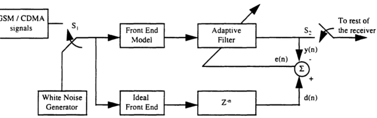
FIGURE 2.20 BLOCK DIAGRAM FOR ADAPTIVE FRONT END EQUALIZATION. THE TERMS IN PARENTHESIS ARE RELATED TO THE GENERAL INVERSE MODELING STRUCTURE ... ... 47
FIGURE 2.21 SOFTWARE IMPLEMENTATION OF FRONT END EQUALIZATION ... ... 50
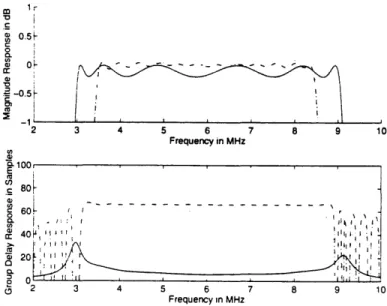
FIGURE 2.22 FREQUENCY RESPONSES: (SOLID LINE): FRONT END MODEL, (DOTTED LINE): 121-TAP ADAPTIVE FILTER AT THE END OF THE TRAINING PERIOD, AND (DASHED LINE): EQUALIZED FRONT END...51
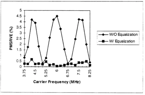
FIGURE 2.23 COMPARISON OF GSM PMSRVE VALUES WITH AND WITHOUT EQUALIZATION. FOR THIS PARTICULAR PLOT, EQUALIZATION IS ACHIEVED USING STEP SIZE OF 0.02, AND ADAPTIVE FILTER LENGTH OF 12 1. ... ... ... . ... ... 52
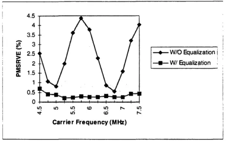
FIGURE 2.24 COMPARISON OF CDMA PMSRVE VALUES WITH AND WITHOUT EQUALIZATION. FOR THIS PARTICULAR PLOT, EQUALIZATION IS ACHIEVED USING STEP SIZE OF 0.02, AND ADAPTIVE FILTER LENGTH O F 12 1... ...54
FIGURE 2.25 LMS MEAN-SQUARE ERROR VS. STEP SIZE ... ... 54
FIGURE 2.26 LMS LEARNING CURVE FOR DIFFERENT STEP SIZES (MU) ... ... 55
FIGURE 2.27 PMSRVE VS. CARIER FREQUENCIES FOR DIFFERENT CHOICES OF M ... 55
FIGURE 2.28 COMPARISON OF PMSRVE VALUES FOR ADAPTIVE FITLERS OF VARIOUS LENGTH (THE STEP SIZE FOR EACH CASE IS SET TO BE 0.002)... ... 56
FIGURE 2.29 COMPARISON OF CDMA PMSRVE VALUES RESULTING FROM USING TWO ADAPTIVE FILTERS WITH DIFFERENT TAP LENGTHS (STEP SIZE FOR BOTH CASES ARE 0.02) ... 56
FIGURE 3.1 BLOCK DIAGRAM OF A GENERAL SPREAD-SPECTRUM COMMUNICATION SYSTEM...59
FIGURE 3.2 MAXIMUM-LENGTH SEQUENCE GENERATOR FOR THE CASE OF M = 3...61
FIGURE 3.3 CONVOLUTION OF SPECTRA OF THE DATA SIGNAL D(T) WITH THAT OF THE PN CODE SIGNAL C(T)63 FIGURE 3.4 NON-COHERENT DIRECT-SEQUENCE SPREAD-SPECTRUM SYSTEM USING BINARY PHASE-SHIFT-K E Y IN G (B P S K ) ... 6 3 FIG URE 3.5 PN CO DE M O DULATION... ... 64
FIGURE 3.7 A NON-COHERENT DELAY-LOCKED LOOP... ... 69
FIGURE 3.8 AUTOCORRELATION FUNCTIONS OF THE A-ADVANCED AND A-DELAYED PN CODES ... 71
FIGURE 3.9 LooP S-CURVE AS A FUNCTION OF E FOR DIFFERENT VALUES OF THE OFFSET A ... 73
FIGURE 3.10 EQUIVALENT MODEL OF DLL ... 74
FIGURE 3.11 NOISE-FREE LINEARIZED MODEL OF DLL ... 75
FIGURE 3.12 TRANSIENT RESPONSE OF A FIRST-ORDER DLL TO A DELAY STEP FUNCTION...76
FIGURE 3.13 MAGNITUDE RESPONSE OF A PERFECT SECOND-ORDER LOOP FOR DIFFERENT DAMPING RATIOS .78 FIGURE 3.14 TRANSIENT RESPONSE TO A CONSTANT CODE RATE MISMATCH...79
FIGURE 3.15 OVERALL SOFTWARE STRUCTURE ... 80
FIGURE 3.16 DISCRIMINATOR CHARACTERISTIC FOR THE SIMULATED DLL (A = 0.5)...81
FIGURE 3.17 FINDPN.M ALWAYS PICKS THE CLOSES CHIP SAMPLE AS ITS OUTPUT. FOR THIS EXAMPLE, THERE ARE 3 SAMPLES FOR EACH CHIP ... 82
FIGURE 3.18 TRANSIENT RESPONSE TO A STEP DELAY INPUT. THE VCO GAINS ARE ONLY TO SHOW RELATIVE V A L U E S ... ... .... ... 83
FIGURE 3.19 RELATIONSHIP BETWEEN FIRST-ORDER DLL TRACKING JITTERS AND LOOP GAIN ... 83
FIGURE 3.20 LINEAR DLL MODEL IN THE PRESENCE OF ADDITIVE NOISE... 85
FIGURE 3.21 SQUARE LOSS (DB) VS. R FOR VARIOUS VALUES OF FD (DB); TWO-POLE BUTTERWORTH FILTER, A = 0.5, NRZ POLAR CODING ... . .. . ... 87
List of Tables
TABLE 2-1 ERROR VALUES FOR VARIOUS CARRIER FREQUENCIES ... ... 29
Chapter 1 : Introduction
Digital Communication systems are often required to operate under statistically unknown, or time varying environment. The desirable features of an adaptive system, namely, the ability to operate satisfactorily in an unknown environment and also track time variations of input statistics, have make it a powerful device to provide the robustness that is desired for all communication systems. Perhaps one of the most well known applications of adaptive system in digital communications is that of channel equalization, where an adaptive filter is used to remove inter-symbol interference (ISI) caused by dispersion in the transmission channel. Of course not just limited to filters, adaptive systems also include closed-loop tracking devices, such as phase-locked loops (PLLs) which play an important role in coherent communications. Although adaptive filters and closed tracking loops are quite different in appearance, they have one basic common feature that is shared by all adaptive systems: an input vector and a desired response are used to compute an estimation error, which is in turn used to control the values of a set of adjustable coefficients. The adjustable coefficients may take various forms, such as tap weights, reflection coefficients, or frequency parameters, depending on the system structure employed. But the essential difference between the various adaptive system applications arises in the manner in which the desired response is extracted.
In this thesis, we are going to present two specific adaptive system applications that are used in modern digital communications systems: adaptive receiver front end correction, and pseudo-noise (PN) code tracking in direct-sequence spread-spectrum (DS/SS) systems using delay-locked loops (DLL). Adaptive front end correction is an example of adaptive filtering, while code tracking using DLL, which is closely related to PLL. is an example of a closed-loop tracking device.
1.1
Receiver Front End Correction Problem
In digital communications an attempt is made to determine which signal from a discrete signal has been transmitted. The transmitter codes and modulates a digital information sequence in a manner suitable for the transmission channel in question. This signal is then transmitted through the channel which will introduce both time dispersion and additive noise. If the communication channel is a cable then this dispersion will have a continuous impulse response which may spread over many intervals, thus causing inter-symbol interference (ISI).1 In the case of a radio channel the dispersion is more likely to be discrete in nature and caused by multipath effects. If the multipath spread exceeds the symbol duration then ISI is once more introduced [21].
After the transmission channel, the signal may encounter another source of distortion at the receiver end. Before this radio frequency (RF) signal can be demodulated, it must be down converted to an appropriate intermediate frequency (IF) through some process such as
superheterodyning. The section of the receiver that controls the process of frequency down-conversion is called the receiver front end. Since the down-down-conversion to IF is normally done through analog means, the front end may introduce some additional distortion to the signal [34]. It is therefore essential for the receiver designer to know whether this additional distortion is significant. First the engineer can formulate a mathematical model for the particular front end to be studied. Often front end can be modeled as a non-ideal band-pass filter similar to a
transmission channel model [21], afterward one can simulate a receiver that incorporates this model to study its front end distortion effect. If the distortion were to be found significant, then a correction filter must be applied to remove the excessive distortion in order to keep the overall receiver performance within specifications. One complication arises in practice is that the front
'ISI is not always undesirable. In the case of Gaussian minimum-shift keying, ISI is allowed as a trade-off for more efficient bandwidth [10].
end characteristic is time varying, due to variations in its down-conversion rate. Accordingly, the use of a single fixed correction filter, which is designed on the basis of average front end
characteristics, may not adequately reduce the distortion. This suggests the need for an adaptive equalizer that provides precise control over the time response of the front end. As Chapter 2 of this thesis will show, a simple linear adaptive filter can be used to achieve this correction.
1.2
Code Tracking in Direct-Sequence Spread-Spectrum Systems
Spread-spectrum communication technology has been used in military communications for over half a century, primarily for two purposes: to overcome the effects of strong intentional
interference (jamming), and to hide the signal from the eavesdropper (covertness). Both goals can be achieved by spreading the signal's spectrum to make it virtually indistinguishable from
background noise [22]. Recently, direct-sequence, a type of spread-spectrum system, has received considerable amount of attention for its possible civilian applications in wireless mobile and personal communications. The key desirable feature in a direct-sequence code division multiple access system (CDMA) is universal frequency reuse, the fact that all users, whether
communicating within a neighborhood, a metropolitan area, or even a nation, occupy a common frequency spectrum allocation [12] -[14].
In a direct-sequence spread-spectrum systems, frequency spreading of an information-bearing (data) sequence is achieved through modulation of a wide-band pseudo-noise (PN) sequence. In order to successfully recover the original data sequence, a synchronized replica of the original transmitting PN sequence must be supplied to the receiver. A solution to the code synchronization problem consists of two parts: code acquisition and code tracking. During code acquisition, the two PN sequences are aligned to within a fraction of a chip in as short a time as possible. Once acquisition is completed, code tracking. or fine synchronization, takes place. The goal of the tracking step is to achieve perfect alignment of the two PN sequences. In this thesis,
we will focus on the code tracking step of the synchronization. Because of the distortion caused by the communication channel, it is unrealistic to expect the delay between the transmitter and receiver to be constant. Therefore, one must solve this problem through the use of an adaptive system. Similar to a phase-locked loop, a delay-locked loop (DLL) can be used to provide code tracking.
1.3
Organization
In the next two chapters, we will examine the front end correction problem and delay-locked code tracking in great detail. The front end correction problem will be covered in Chapter 2. First half of the chapter presents a study on front end distortion to both GSM and CDMA signals. Then the second half present a front end correction scheme that uses a linear adaptive filter together with computer simulation results. Chapter 3 addresses the application of delay-locked loops for PN code tracking. Simulation results of a first-order delay-order loop is presented. Chapter 4 provides a summary for the thesis by introducing a general adaptive system model that encompasses both applications being discussed so far. It also explores future research possibilities in the area of adaptive system applications.
Chapter 2: Front End Correction Problem
The remainder of the thesis describes several applications of adaptive processing in digital communications. This chapter will cover one of the applications -adaptive front end
equalization. The description of the front end correction problem is in two parts. The first part (2.1) will present a study of the effect of distortion in a front end used in a high precision telecommunication measurement device. This study shows that the distortion introduced by the front end is excessive and must be removed using a correction scheme. Then in part two (2.2), a front end correction scheme that uses least-mean-square (LMS) algorithm driven adaptive transversal filter is presented. The results will show that by using appropriate design parameters, distortion can be corrected with reasonable cost.
RF Signal IF Signal
Mixer IF Filter
Receiver Front End
Figure 2.1 A general front end structure
As depicted in Figure 2.1, a front end is the section of a receiver that controls the process of down-conversion of radio frequency (RF) signal to an appropriate intermediate frequency (IF) through a process such as superheterodyning. To illustrate, Figure 2.2 shows a superheterodyne receiver commonly used in AM radio broadcasting. In this receiver, every AM radio signal is converted to a common IF frequency, say
fir.
This conversion allows the use of a single tuned IF amplifier for signal from any radio station in the frequency band. The IF amplifier is designed to have a certain bandwidth centered around fIF, a bandwidth which matches that of the transmittedsignal. So in this case the IF amplifier can be seen as the cascade of an IF filter and an amplifier. Since down-conversion to an IF signal is normally done through analog means, the front end inevitably introduces distortion to the signal. This distortion may not have much effect in an AM radio receiver, but it may adversely affect a high resolution, high fidelity telecommunication measurement device. If so, then an error correction scheme must be applied. Through prior work done on the subject, a model for the front end has already been formulated. It was modeled as a six-pole Chebychev type I band-pass filter. This thesis examines use of this model to (1)
characterize the distortion by applying simulated GSM and CDMA data signals to this model, and (2) recommend a correction scheme if the distortion was found to be excessive according to the product specifications.
IF Amplifier A
Oscillator
Figure 2.2 A superheterodyne receiver commonly used for AM radios
2.1
Front End Distortion Study
Both GSM and CDMA simulations are based on a front end that is modeled as a Chebychev Type I band pass filter with approximately 6 MHz bandwidth. Its prototype analog low pass filter has six specified poles:
-- 0.092
- 0.252±
±
0.966j
0.707j
-
0.344 ± 0.259
j
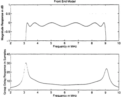
With specified sampling frequency, and above pole values, a MATLAB M-file was written to implement the corresponding digital band pass filter using bilinear transformation. Figure 2.3 shows the frequency response of this digital band pass filter based on these pole values and a
sampling rate of 27 MHz. As shown in Figure 2.3, two potential sources of distortion exists: One comes from the ripple in the pass band of the model, and the other stems from the non-constant group delay response visible in the pass band. As shown in the results and analysis
section (2.1.1.4 and 2.1.2.4), the ripple in the pass band dominates the distortion.
Front End Model
0.5--1 2 3 4 5 6 7 8 9 10 Frequency in MHz c i a40 E n 30
~0
2 3 4 5 6 7 8 9 10 Frequency in MHzFigure 2.3 Front end modeled as a band pass filter with 6 MHz center frequency. 6 MHz bandwidth, and 0.2 dB ripple in the pass band: (top) magnitude response, (bottom) group delay
response
-This value should become clear after discussion of the simulation parameters used for GSM and CDMA in the next two sections
To study the effect of this front end model on GSM and CDMA data signals, simulation programs were written to implement the transmitter-receiver structures that were representative of GSM and CDMA standards. Of course, incorporating every existing feature of these standards into our simulations would be both time consuming and unnecessary. Instead, we will only concern ourselves with the features that are pertinent to the study at hand. To elaborate, we will consider the bandwidth of the signal to be an important factor in deciding the extent of the distortion it can tolerate. For a narrow band signal. depending on the frequency location of the
signal with respect to the front end, different distortion may result. On the other hand, for a wide band signal, the distortion would be approximately an average of distortions experienced by all the narrow band signals within the wide band range. It would not be unreasonable to assume that narrower bandwidth signals may escape the distortion effects of the front end better than the wider ones. In cases of GSM and CDMA, the former would be relatively narrower than the latter. The code spreading process is the major factor of the wider band appearance of the CDMA signal. Different modulation schemes used for GSM and CDMA further contributes to this bandwidth discrepancy. As we shall see later, Gossip minimum shift keying (GMSK), the modulation scheme used by GSM. is very spectrally efficient. In contrast, the modulation scheme used by CDMA is not as efficient. Features such as these must, therefore, be incorporated into the simulations, while the rest can be safely ignored without affecting the results. In the next two sections we will present the simulations done for GSM and CDMA in detail.
H (j to
Front End Frequency Response
Simulated GSM or CDMA Signal Response
f
Figure 2.4 Using different carrier frequencies, signal can be placed over various frequency bands of the front end in order to study its behavior
After the transmitter-receiver structures are put into place, simulated data signals for both GSM and CDMA can be easily generated. The features of the instrument, whose front end is being studied here, require the placement of data signals over various frequency regions near the center of the front end. In order to measure distortion in these frequency regions, three sets of data signals will be generated for GSM and CDMA simulation as shown in Figure 2.4 These
signals, labeled "1", "2" and "3", differ only in their carrier frequencies, which in turn determine their corresponding placements in the frequency domain. The random data bits used to generate them are identical for all three cases, a fact that will aid in better analysis of the relationship between distortion and frequency placements. For both simulations, the three carrier frequencies are chosen such that the lowest and the highest would correspond to, respectively,
-1MHz and +1MHz offset from the center of the front end pass band (labeledfFE in Figure 2.4). Data Signal A
110Front End Model Demodulator Constellation APercent
Vector
- Error Generator Reference
Figure 2.5 Basic experiment setup
In order to generate a measure of the distortion for each of the three data signals shown in Figure 2.4. two different receiver outputs will be generated depending on the data path the input
takes (illustrated in Figure 2.5). The output generated using the dotted line path is considered to be the reference output, or the distortion-free output, since the input data reaches the
demodulation stage without passing through the front end model. The other output is obtained by passing the input data along the solid line, which goes through the front end model. This output will reflect the front end distortion effects, and is appropriately labeled as the corresponding distorted output. By comparing this output with its reference output, we can obtain the magnitude of the distortion.
To be consistent with the distortion measurement adopted by the instrument specifications, we are going to use percentage mean-square-root vector error (PMSRVE) to measure the extent of the distortion. Our simulated receiver will produce both an in-phase (I) and a quadrature-phase (Q) component. By plotting the correspond I and
Q,
we can create what is called a constellation diagram. Designating I andQ
as y- and x-axis, respectively, we can treat any point in the constellation as a two dimensional vector. Comparing outputs thus becomes equivalent to comparing corresponding vectors in the two constellation plots created for the twoinputs. PMSRVE is thus defined by the following:
. (It -I t,) +(Qi
-Qi.
re)
2 +Qi--,V IL.,f + Q i.,e,
PMSRVE =N N x 100 (Equation 2.1)
where N is the total number of vectors to be considered for the calculation of PMSRVE, Ii and
Q,
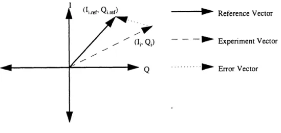
are the components for the i-th distorted vector, and Ii.ref and Qi.rer are the components for the i-th reference vector. Figure 2.6 illustrates the error vector, the dotted line, between vector (I,,Qj)
and--Q- Reference Vector
i, Qi) - Experiment Vector
Q ... Error Vector
Figure 2.6 Looking at vector error in terms of a constellation diagram. A vector is made up of a pair of symbols from I and
Q,
respectively.Using PMSRVE values, we are able to get a sense of the extent of the distortion introduced by our front end model. When values exceed those given in the specification sheet, the distortion will
be considered excessive, and possible correction schemes must be addressed next. In the next two sections we are going to cover the GSM and CDMA simulation details. As the results of both simulations will show, the front end distortion indeed causes performance degradation that exceeds requirement. leading to the introduction of a correction scheme using least-mean-square (LMS) adaptive filtering. The results of using such a scheme will then be presented to show that FIR adaptive filtering does offer, with a reasonable cost, a robust error correction solution to the problem at hand.
2.1.1
GSM Simulation
While the last section gives an overall description of the approach we take to study the front end distortion, this section will present in detail the simulation setup for the GSM case. Specifically
we are going to present the parallel GMSK transmitter that is used to produce the required GSM data signal, along with the parallel GSMK receiver that is used to produce the constellation plots
later used during PMSRVE calculations. But prior to that, we will give an overview of
continuous phase modulation (CPM) of which GMSK is a subtype, which will help us to better understand the transmitter-receiver. And finally, we will present the simulation results that will show, as in the CDMA case, that the magnitude response of the front end introduces most of the error, and not its group delay response (non-constant group delay corresponds to nonlinear phase response). And the extent of the distortion depends heavily on the frequency location of the signal with respect to the front end response. More importantly, without any correction scheme, the front end model clearly introduces excess distortion.
2.1.1.1 Continuous Phase Modulation
While digital communication has grown as a field, one digital communication method known as continuous phase modulation (CPM) has become a popular method of transmitting digital information in a mobile radio environment. In applications such as mobile radio and satellite transmission, where power must be conserved, amplifiers need to operate in a saturated and nonlinear region for maximum efficiency [1]. Because of its constant envelop, CPM is less affected by nonlinear RF amplifiers than the non-constant envelop schemes such as quadrature amplitude modulation (QAM) [2]. Non-constant envelop modulation schemes are also more susceptible to the effects of fading than constant envelop schemes [3]. The continuity of the phase inherent in a CPM signal also reduces bandwidth requirements in comparison to discontinuous phase modulation such as quadrature phase shift keying (QPSK) [9] [5]. While QPSK can be bandlimited before transmission to reduce its out-of-band power, the resulting time varying envelope may cause high error rates for certain symbol transitions [3]. As with most engineering choices. CPM is chosen as a compromise for the mobile radio environment which requires digital transmission, efficient amplifiers, and limited bandwidth.
CPM can be sub-divided into a number of specific types, providing choices between bandwidth. receiver complexity, and power [5] [6]. The general form of a transmitted CPM signal is
s(t,U) = Fý cos(2nft +O(t,a)
+O)
(Equation 2.2)=(t,)
= 21thi
cXq(t
- iT) (Equation 2.3)where f, is the carrier frequency, T is the symbol duration. 0,, is the arbitrary phase, and b(t,U) is
the phase information. The phase information is determined by a sequence of M-ary data symbols, a = a,,.a, .... with ao = +1.3,...,±(M - 1). The parameter h is known as the
modulation index and plays a role similar to the frequency deviation ratio in analog frequency modulation by scaling the phase signal representing the transmitted information.
CPM systems are partly classified by the form of q(t), the phase response, which is denoted as
q(t) = g(t)dt (Equation 2.4)
where g(t) is causal and known as the pulse shape of a CPM system. The final value of q(t) is always set to 1/2.
The pulse shape, g(t), has a direct effect on the bandwidth, receiver complexity, and the likelihood of correctly detecting the transmitted data. Each g(t) is primarily characterized by its shape and duration. Longer and smoother pulses reduce the bandwidth of the CPM signal while making symbol detection more difficult. As the duration of g(t) increases past one symbol period, controlled intersvmbol interference (ISI) is introduced into the signal. This ISI blurs the phase response of each symbol. making signal detection more difficult. A prefix or suffix, "L", may be
added to the name of a modulation. When present, it will indicate that the corresponding g(t) is truncated to [0, LT]. When L = 1, the CPM system is known as a full response system. When L >1, the system is known as a partial response system. This distinction is important because only partial response systems can create controlled ISL although they usually have better bandwidth performance. Figure 2.7 illustrates an equivalent representation of the CPM signal as a frequency
modulation (FM) system where input symbols are convolved with a filter having the pulse shape, g(t), as its impulse response [6].
Figure 2.7 An alternative representation of CPM using frequency modulation
2.1.1.2 Gossip Minimum Shift Keying
The modulation scheme adopted by GSM is Gossip minimum shift keying (GMSK), which is a type of CPM. In the GMSK that we are going to consider for the implementation of GSM transmitter/receiver structure, g(t) is a Gossip pulse convolved with a rectangular pulse of unit area and one symbol duration. Specifically, as given in [7], the modulating data values o(X, as represented by Dirac pulses, excite a linear filter with impulse response defined by:
g(t) = h(t)* rect(t / T) (Equation 2.5)
where * means convolution, T is the symbol duration, the function rect(t) is defined by:
I
< t
rect(t)
=
-
2T
(Equation 2.6)
and h(t) is defined by:
h(t)
-e/2a,
T(Equation 2.7)
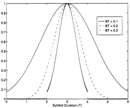
where a = 2BT , and B is the 3 dB bandwidth of the filter with impulse response h(t). The shape
of g(t) is parameterized by the time-bandwidth product, BT, where smaller BT values indicate more spreading in the pulse shape (see Figure 2.8). [7] further sets the value of BT at 0.3. The simulation will be based on the values given in [7]. Notice that the response for the ideal Gossip filter is infinite in duration, and thus the GMSK in our simulation must be a truncated signal. Fortunately. the amplitude of GMSK with BT = 0.3 at time instants more than two symbol periods away from its center will be very small, resulting in little effect from the truncation. For smaller BT values, however, such as BT = 0.1, the truncated pulse duration may need to be extended to perhaps six or seven symbol periods before the amplitude of g(t) becomes efficiently small. In any case, the inter-symbol-interference (ISI) will be present.
In the transmitter-receiver structure we are going to simulate, we only considers binary modulation, i.e., M = 2, thus making the area of cj equal to +1 . Larger values of M significantly increase the complexity of the receiver. Further more, we will the modulation index. h, to the value of 1/2 (see Equation 2.3) which allows for highly simplified receivers [8]. In the case of full response systems, the value of h = 1/2 is the minimum possible value for the two signals produced by I and -1 to be orthogonal-hence the name minimum shift keying [9].
0. 0. 0. 0. 0. O. 0 0 0 0 1 2 3 4 5 6 Symbol Duration (T)
Figure 2.8 Impulse response of g(t) for GMSK with different BT values
2.1.1.3
GMSK Transmitter-Receiver
The simulation program for the transmitter-receiver structure incorporates several assumptions. We assume that the transmission channel is a perfect all pass system without any additive noise terms, and the receiver uses a coherent demodulation method that is capable of both perfect phase recovery and exact timing synchronization.
Now we are going to consider some of the parameters that are used in the simulation. The first issue is the sampling rate. A low sampling rate is desirable to reduce the amount of
processing, but a high sampling rate reduces the effects of aliasing. Based on the power spectrum given in Figure 2 of [10], and a symbol rate of 271 kbits/sec specified for GSM [7], the GMSK signal will be attenuated by 60 dB at approximately 340 kHz from its center frequency.
Therefore, we will assume that the signal has a bandwidth of 680 kHz (this is a lot smaller than the bandwidth of the signal to be considered for the CDMA case, which we will present in the next section). This dictates the lowest permissible sampling rate of 1360 kHz. For our
simulation, we are going to use an odd integral number of samples per symbol. so that at the receiver end we will have an unambiguous choice for symbol timing. As stated in the previous section, we are going to use a band pass filter of 6 MHz bandwidth, thus the sampling rate has to be much higher. We pick, rather arbitrarily, the number of samples per symbol to be 99. This gives a sampling rate around 27 MHz. The symbols used in the simulation are binary random
+1 's.
Since GSM uses partial response system [7], i.e., L > 1 (see discussion in the CPM section), there exists finite controlled inter-symbol-interference (ISI). For the simulation, we are going to set L = 2. It is a compromise between bandwidth performance and controlled ISI. In other words. we are going to use g(t) with duration of 2 symbol periods (T). The time-bandwidth product, BT, is always set to be 0.3.
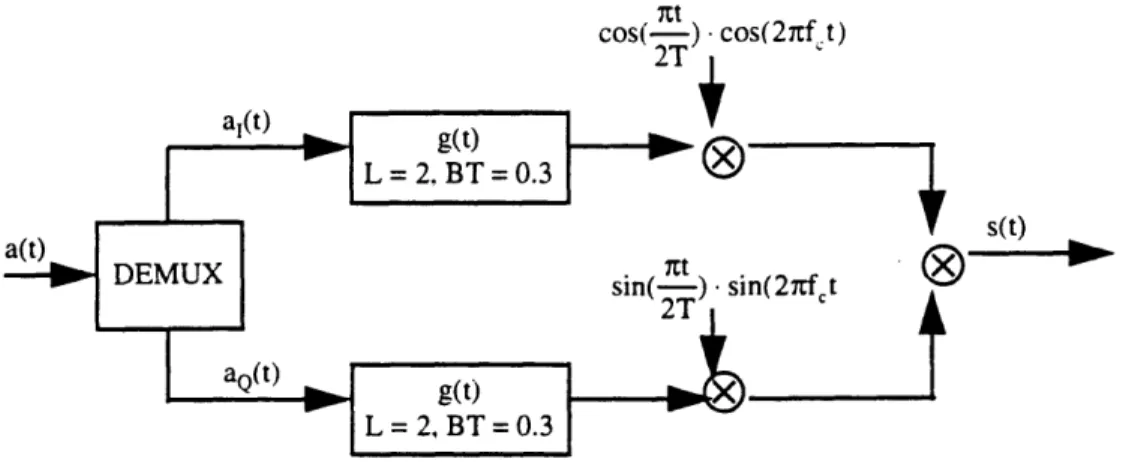
Incorporating all these parameters, Figure 2.9 shows the block diagram of the parallel GMSK transmitter used for the simulation. Here we take the approach outlined in [9]. The only difference between MSK and GMSK is the addition of a Gossip pulse shaping filter g(t) used in the latter. As proved in [9], a MSK signal can be thought of as a special case of offset quadrature phase shift keying (OQPSK) (We are going to talk more about QPSK and OQPSK in our CDMA simulation). The only difference is that instead of using rectangular pulse shapes as in OQPSK, MSK uses sinusoidal pulses, which is the reason for the appearance of cos( tt) and sin( )
2T 2T Both al(t) and aQ(t) are rectangular pulse stream corresponding to the even and odd bits in the input symbol. All the pulses has duration of 2T. Also note that I channel leads
Q
channel by one symbol duration. T.ntt
cos(-) -cos(27tf. t) 2T
Figure 2.9 Block diagram for the GMSK parallel transmitter: BT = 0.3, sampling frequency = 27 MHz Xt cos(-) -cos(2nf•.t) Eye Diagram & Constellation
Figure 2.10 Block diagram for the GMSK parallel receiver: BT = 0.3, sampling rate = 27 MHz
For the receiver, we assume perfect recovery of the phase, thus committing the use of a phase-locked loop. The parallel receiver shown in Figure 2.10 downconverts the received signal r(t) into an inphase (I(t)) and quadrature (Q(t)) branch. While a low-pass filter could be used to remove the high frequency components, the predetection filter sufficiently attenuates the high frequency components to avoid the use of this extra filter. The time domain shape of the predetection filter is equivalent to a Gossip pulse convolved with a rectangular pulse, which is like g(t) itself. Since BT = 0.3 is very close to the level found in [10] for optimum bit error rate (BER) performance, the same g(t) is also used in the receiver. One should note. however, that the
value of BT = 0.3 for the predetection filter is almost independent of the BT value used in the transmitter.
2.1.1.4 Simulation Results and Analysis
GMSK transmitter/receiver is simulated using MATLAB with data bits generated by a random number generator. As we have stated, the simulated GSM signal would be generated using three different carrier frequencies so that we can study the relationship between the magnitude of the distortion and frequency. A single set of data bits is used throughout the whole simulation to ensure that we can analyze the results considering minimum number of variables. Since both the front end model and the data bits used are identical in all three cases, any difference in distortion behavior noticeable at the receiver end can be solely ascribed to the nonidealness of the front end response. The measure for the distortion is provided by PMSRVE values as described in Equation 2.1.
Since the center frequency of the front end is approximately around 6 MHz, with the assumption that most signals we are interested in will be concentrated around that frequency, we choose 5Mhz, 6 MHz, and 7 MHz to be the three carrier frequencies to be used in the simulation. Three percent error values are calculated based on Equation 2.1, and they are listed in Table 2-1. We can easily notice that the values are rather different depending on the carrier frequency being used: from 0.29% at 5MHz, to 4.5% at 6MHz. This means that the amount of distortion created by the front end depends heavily on the frequency location of the data signal. This frequency dependent behavior can be easily explained if we look closely at the frequency response of the front end model shown before in Figure 2.3, where the group delay response over most of the pass band (excluding where it is near the edges) can be characterized as flat, the magnitude response clearly shows ripples as large as 0.2 dB. As we showed before, the bandwidth of the GSM signal is around 680 kHz. With the particular carrier frequency of 5MHz. most of the data is
concentrated around the part of the ripple that is probably the closest to the ideal 0 dB line; this explains why the error value at that location is small. On the other hand, for the carrier frequency
of 6MHz, the data will be sitting near where the magnitude response of the front end is at its worst, thus the resulting high PMSRVE value.
Table 2-1 Error values for various carrier frequencies
Figure 2.11 GMSK
0.1 0.2 0.3 0.4
constellation diagram: dotted line represents undistorted data, while "+" represents the one using front end corrupted data.
03[ 02-0.1i 01 -0 •1 -0. 2 --o.31 -04 -0.3 -0.2 -0.1 0 a
Figure 2.12 GMSK eye-diagram: solid line is the undistorted version, while the dotted line is from corrupted data. Number of samples per symbol is 99.
This distortion, if not removed, will cause significant loss in performance in the decision making stage of receiver. Specifically, we will see that this distortion can be translated into the shift in the constellation plot, or equivalently, the narrowing of the eye opening in the eye-diagram. Using I and
Q
data, we can easily plot the constellation. Figure 2.11 shows two superimposed plots. The dotted one is the undistorted version, while the one plotted using "+" is generated using data received after passing through the front end at 6 MHz. For the 6 MHz one, there are decreases in magnitude for both I andQ.
Since we are dealing with binary ±1 symbols, this brings the + side closer to the -side, thus distinguishing them correctly becomes harder. This effect can also be seen in an eye-diagram shown in Figure 2.12, where the solid line represents the undistorted data, and the dotted line the corrupted data. For a high resolution GSM measurement device, the largest percent error it can tolerate is less than 0.3% 3 . Thus some kind of correction scheme mustbe devised to remove this distortion. Later we are going to show that using a linear phase FIR adaptive filter, this kind of distortion can be easily removed.
2.1.2
CDMA Simulation
Similar front end distortion studies are performed for the simulated CDMA data signals. To generate CDMA signal, we have to first develop a sufficient model for the system. In contrast to GSM, which uses the conventional narrow band communication technology, CDMA is based on spread spectrum signaling, which is used extensively in military communications to overcome strong intentional interference (jamming), and to prevent eavesdropping. Both goals can be achieved by spreading the signal's spectrum to make it virtually indistinguishable from
background noise. The particular CDMA signal we are going to simulate here is based on direct-sequence spread spectrum signaling, where spreading is achieved by modulating the conventional bandlimited signal with a long pseudo-random code. CDMA is a complicated system where it would be impractical to include every single feature in our model. Fortunately, as we will show later, we need not concern too much about the spread spectrum technical details for the purpose of this simulation. A conventional QPSK transmitter, provided with appropriate data rate, should be sufficient to generate a data signal that includes the necessary features adequate for the study of distortion effects of the front end model on CDMA. A more extensive discussion on spread spectrum system will be given in the next chapter.
The remainder of the section is structured as follows. First we are going to give a very brief description of a direct-sequence CDMA system. Based on that, we are going to select a small number of important features that are going to be included into our simulation model by making appropriate assumptions. The most important feature to be included in our model of CDMA is its much wider signal bandwidth compare to that of GSM. Second we are going to present a QPSK transmitter-receiver structure that is used to both generate the simulate CDMA signals and derive the their outputs to be used for the PMSRVE calculations. At this point it should become apparent that the main reason for the CDMA signals to experience more severe distortion stems from its wider bandwidth. Based on the results of the previous GSM study, we
can safely say that correction should be necessary to keep the receiver performance level within specification.
2.1.2.1 CDMA
As is well known, the two most common multiple access techniques are frequency division multiple access (FDMA) and time division multiple access (TDMA). In FDMA, all users transmit simultaneously, but use disjointed frequency bands. In TDMA, all users occupy the same radio frequency (RF) bandwidth, but transmit sequentially in time. When users are allowed to transmit simultaneously in time and occupy the same RF bandwidth as well, some other means of signal separation at the receiver must be available; CDMA, or code division multiple access, provides this necessary capability.
A simplified block diagram of a direct sequence CDMA system is shown in Figure 2.13. (Direct-sequence spread spectrum system will be discussed in the next chapter when we cover delay-locked loops. Interested readers can also consult several other references on the subject
111] -[13].) Here the message d,(t) of the i-th user, in addition to being modulated by the carrier
cos(oot + O,), where 0, is the random phase of the i-th carrier, is also modulated by a spreading
code waveform pi(t) that is specifically assigned to the i-th user, hence the name code division. This code modulation translates into spectrum spreading in the frequency domain because the code rate, or chip rate, is usually much higher than the underlying data rate. To see this, for instance before the spreading, the signal has a one-sided bandwidth of B, where B is the data rate. But after code modulation, the signal bandwidth becomes Bc, where B, is the chip rate (which is much greater than B). Now this time, the signal that has to pass through our front end model has a much wider bandwidth than what we saw for the GSM case. So we would expect different levels of distortion at the receiver output. The spreading code waveform for the i-th user is a pseudo-random (PN) sequence waveform that is approximately uncorrelated with the waveforms
assigned to other users. This property enables the receiver to distinguish the different data sent by multiple users. There are a lot of technical issues involved in the design of CDMA systems [11 ]. For the present simulation, we are able to safely to simplify most of the details.
di(t) p,(t) cos(co0 t + 01)
di(t) pi(t)
dN(t) PN(t
I Pi(t) cos(coot + 01)
ith User Demodulator
Figure 2.13 General direct-sequence CDMA system
2.1.2.2 Simulation Setup
Similar to what we have done for the GSM simulation, we are going to assume that the only source of distortion is the front end itself. This leads to the assumptions of an ideal channel and a receiver which performs perfect carrier recovery. In addition, since we are dealing with CDMA, which is based on a spread spectrum system. we are also going to assume perfect code synchronization at the receiver end (code synchronization is the topic of next chapter).
Based on the model illustrated in Figure 2.3. the amount of distortion that front end can inflict on a signal will be closely related to two parameters associated with the signal. namely its frequency location and bandwidth. We have already seen the close relationship between
frequency location and distortion from the GSM simulation results. We expect the similar
relationship holds for the CDMA signals. Since CDMA signals has a much wider bandwidth than that of GSM, we are going to use the CDMA simulation to help us better understand the
relationship between distortion and signal bandwidth, which can not be observed just from the GSM simulations. The bandwidth difference is mainly caused by the additional code spreading
process used in CDMA systems. In addition, less spectrally efficient modulation scheme used by CDMA also widens this bandwidth discrepancy. For the purpose of our simulation, we can further simplify the simulation model from what is shown in Figure 2.13. We are only going to consider the single-user case, since its signal has the same bandwidth as that of a multi-user signal, which is also much more complex. The code spreading process is simulated using random data bits whose rate equals the code rate (also called chip rate) of 1.2288 MHz, which is often used for CDMA systems [14]. The transmitter-receiver structure used in the simulation is based on quadrature phase-shift-keying (QPSK), a common modulation scheme for CDMA [12]. Regarding sampling rate, we are going to choose the number of samples per chip such that the overall sampling rate is at par with that used in the GSM case. This would ease the comparison of their distortion results so that we can better understand the relationship between distortion and bandwidth. 0.6 0.4 0.2 0 -0.2 -0 4 0 5 10 15 20 25 30 35 40 45 50
Figure 2.14 QPSK eye diagram: 23 samples per chip
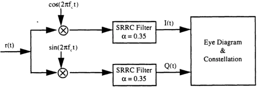
2.1.2.3 QPSK Transmitter/Receiver
The block diagrams for the parallel QPSK transmitter and receiver are shown in Figure 2.15 and Figure 2.16. Compared to the GMSK transmitter, there is no time offset between I and
olI
-0.2 -0.4 _,'3 R = O0C _ _Q
arms in the QPSK transmitter. Instead of using a Gossip filter as for GMSK, this transmitter uses a square root raised-cosine (SRRC) filter as the base-band shaping filter. The same filter is also used by the receiver after the carrier is removed. The desired magnitude response is given by[14]:
IH(f)l =
1-a 2T 1-oa -a f _+a l+a
(Equation 2.8)
2T 2T
l+a
f>2T 2T
where T is the symbol period, which in this case is 1/1.2288 msec, a is the roll-off factor, which determines the width of the transition band, and is set to be 0.35 [14]. Figure 2.14 QPSK eye diagram: 23 samples per chipshows a eye diagrams generated using this transmitter-receiver structure.
cos('2rfCt)
s(t)
SRRC Filter it ) a= 0.35 SRRC Filter
ri35
U
= .
Eye Diagram & ConstellationFigure 2.16 QPSK receiver used in the CDMA simulation
2.1.2.4 Results and Analysis
The QPSK transmitter/receiver is simulated using MATLAB with data bits generated by a random number generator. Similar to what we have done for the GSM case, three sets of simulated CDMA signal are generated using three different carrier frequencies so that we can study the relationship between the magnitude of the distortion and frequency. A single set of data bits is used throughout the whole simulation to ensure that we can analyze the results with a minimum number of variables. Since both the front end model and the data bits used are identical in all three carrier frequencies. any difference in distortion behavior noticeable at the receiver end can be solely ascribed to the different front end response at various frequency locations. The measure for the distortion is provided by PMSRVE values as described in Equation 2.1.
Like in the GSM case, the center frequency of the front end is approximated around 6 MHz, with the assumption that most signal we will be interested in will be concentrated around the that number, we choose 5Mhz. 6 MHz, and 7 MHz to be the three carrier frequencies to be used in the simulation. Three error values are calculated based on Equation 2.1. and they are listed in Table 2-2. Similar to the error values in Table 2-1, the error values are closely related to the frequency placement of the signal with respect to the ripples in the front end magnitude response. Since the CDMA signal has a much wider bandwidth, the effect of the front end is
averaged over the band occupied by the signal. That is why at 6MHz, the error value is actually smaller for CDMA than that of GSM.
0.6 X. 0.4 0.2 0- -0.2--0.4 * K x -0.6 -0.4 -0.2 0 0.2 0.4 0.6
Figure 2.17 QPSK constellation diagram: ' x' represents undistorted data, while "" represents front end corrupted data
Figure 2.17 shows two superimposed constellation plots generated using data of 6MHz carrier frequency, where the cross represents the undistorted constellation, and the dot represents the front end corrupted version. Clearly both I and
Q
for the distorted version show smaller values than their distortion free counterparts. Since we are dealing with binary ±+1 symbols, this brings the + side closer to the -side, thus distinguishing them becomes more difficult. An error of 3.79% for the 6MHz case in Table 2-2 is not acceptable. Some kind of correction scheme must be devised to remove this distortion. In the next section, we are going to introduce an errorcorrection solution that uses a FIR adaptive filter. We are going to show that when the adaptive filter is properly set, it can be very effective in removing the distortion.
2.2
Adaptive Front End Equalization
The results thus far clearly show that the distortion introduced by the front end on both GSM and CDMA signals is well above what specifications allow, and corrections must be applied to remove the distortion. One might consider using a fixed correction filter such that when it is cascaded with the front end, the overall response would more or less resemble an ideal allpass system with both gain and group delay being constant. However, this is not a feasible approach. Modeling the front end as a fixed band pass filter (shown in Figure 2.3) was solely for the purpose of characterizing the extent of its nonidealness. Specifically, we would like to know from the model what is the largest amount of distortion it can afflict on the signal that passes through it. Based on that information, we can then make a decision about whether correction will be needed. In real time operation, however, the front end displays a slow4 time-varying response, with its exact shape at any time instant unknown. The model is simply an approximation of its average response. So a fixed correction filter may work during one time period, but fail at the next. Clearly we can not keep on replacing new correction filter for the old one, unless we take a adaptive system approach. Specifically we propose the use of a linear adaptive filter that is able to track the slow changes of the front end response, so that the overall response of their cascade would be all-pass.
After we give a brief overview of the concept of adaptive filtering, we are going to present a linear adaptive equalization structure that can be applied to the front end, and describe the least
mean-square (LMS) algorithm that can be used to derive the correction filter. And finally, we are going to present the results of the simulation. As they will show, by choosing appropriate design parameters, front end distortion can be successfully removed for both GSM and CDMA signals.
2.2.1
Adaptive Filters
In the statistical approach to the solution of the linear filtering problem, we assume the availability of certain statistical parameters, such as the mean and correlation functions, of the useful signal and unwanted additive noise. The requirement is then to design a linear filter with the noisy data as input so as to minimize the effects of noise at the filter output according to some statistical criterion. A useful approach to this filter-optimization problem is to minimize the mean-square value of the error signal, which is defined as the difference between some desired response and the actual filter output. For stationary inputs, the resulting solution is commonly known as the Wiener filter, which is said to be optimum in the mean-square sense.
The design of a Wiener filter requires a priori information about the statistics of the data to be processed. The filter is optimum only when the statistical characteristics of the input data match the a priori information on which the design of the filter is based. When this information is not known completely, however, it may not be possible to design the Wiener filter or else the design may no longer be optimum. A straightforward approach that we may use in such situations is the "estimate and plug" procedure. This is a two-stage process whereby the filter first
"estimates" the statistical parameters of the relevant signals and then "plugs" the results into a nonrecursive formula for computing the filter parameters. For real-time operation, this procedure has the disadvantage of requiring excessively elaborate and costly hardware. A more efficient method is to use an adaptive filter. An adaptive filter is self-designing in that it relies for its operation on a recursive algorithm, which makes it possible for the filter to perform satisfactorily in an environment where complete knowledge of the relevant signal characteristics is not available. Such is the case with our front end, which has, to some extent, unknown frequency response. The algorithm starts from some predetermined set of initial conditions, representing complete ignorance about the environment. Yet, in a stationary environment, after successive iterations of the algorithm, the filter will converge to the optimum Wiener solution in some
statistical sense. In a nonstationary environment, the algorithm offers a tracking capability, whereby it can track time variations in the statistics of the input data, provided that the variations are sufficiently slow. Again, fortunately, our front end offers this feature.
As a direct consequence of the application of a recursive algorithm, whereby the
parameters of an adaptive filter are updated from one iteration to the next, the parameters become data dependent. This, therefore, means that an adaptive filter is a nonlinear device in the sense that it does not obey the principle of superposition. In another context, an adaptive filter is often referred as linear in the sense that the estimate of a quantity of interest is obtained adaptively as a linear combination of the available set of observations applied to the filter input.
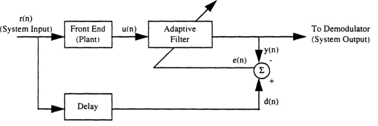
The operation of an adaptive filter involves two basic processes: (1) a filtering process designed to produce an output in response to a sequence of input data, and (2) an adaptive process, the purpose of which is to provide a mechanism for the adaptive control of an adjustable set of parameters used in the filtering process. While the filtering process depends its operation on its filter structure, the adaptive process is governed by a adaptive algorithm. Thus a general adaptive filter can be presented as in Figure 2.18, where u(n) is the input, d(n) is the desired response,
d(n
Un) is the estimate of the desired response given the input data that span the space Un up to and including time n. The front end equalization method that we are going to simulate here uses a type of filter structure called the transversal filter, and a particular adaptive algorithm called the least mean-square (LMS) algorithm.u(n)
+
d(n)
Figure 2.18 Block diagram of a general adaptive filter.
2.2.1.1 Transversal Filter
The choice of a structure for the filtering process has a profound effect on the operation of a adaptive filter as a whole. There are mainly three types of filter structures that distinguish themselves in the context of an adaptive filter with finite memory or, equivalently, finite impulse response (FIR). They are transversal filter, lattice predictor, and systolic array. We choose transversal filter as our filter structure because it is the most straight forward of the three for software simulation, and also it is usually the least expensive for hardware implementation. If the reader is interested in learning more about the other two types of filter structures, [15] provides a good overview.
The transversal filter, also referred to as a tapped-delay line filter, consists of three basic elements, as depicted in Figure 2.19: (1) unit-delay element (square box), (b) multiplier (large circle), and (c) adder (small circle). The number of delay elements used in the filter determines the duration of its impulse response. The number of delay elements, shown as M -1 in Figure
2.19. is commonly referred to as the order of the filter. In this figure, the delay elements are each identified by the unit-delay operator z-'. The role of each multiplier in the filter is to multiply the
tap inputs (to which it is connected) by a filter coefficient referred to as a tap weight. Thus a multiplier connected-to the k-th tap input u(n - k) produces the inner product wku(n -k), where Wk
is the respective tap weight and k = 0, 1 . . . , M -1. Here we assume that the tap inputs and therefore the tap weights are all real valued. For complex values, in place of wk should be its complex conjugate. The combined role of adders in the filter is to sum the individual multiplier outputs (i.e., inner products) and produce an overall filter output. For the transversal filter described in Figure 2.19, the filter output is given by
M-I
y(n)= I wku(n - k) (Equation 2.9)
k=O
which is a finite convolution sum of the filter impulse response { w) } with the filter input { u(n) }. One thing worth noting is that an FIR filter is inherently stable, which is characterized by its feedforward only paths, unlike an infinite impulse response (IIR) filter which contains feedback paths. This is also one reason we choose a FIR filter as the structural basis for the design of adaptive filter. Now we have settled the filter structure, what kind of guarantee do we have on that { wn } are going to converge eventually? To answer that question, we have to know the adaptive algorithm that is used to control the adjustment of these coefficients
Least Mean-Square (LMS) Algorithm
A wide variety of recursive algorithms have been developed in the literature for the operation of adaptive filters. In the final analysis, the choice of one algorithm over another is determined by various factors. Some of the important ones are (1) rate of convergence, (2) tracking ability, and (3) computational requirements. Rate of convergence is defined as the number of iterations required for the algorithm, in response to stationary inputs, to converge "close enough" to the optimum Wiener solution in the mean-square sense. A fast rate of convergence allows the algorithm to adapt rapidly to a stationary environment of unknown statistics. The tracking ability of an algorithm applies when an adaptive filter is operating in a nonstationary environment. It is more desirable if the algorithm has the ability to track statistical variations in the environment. Computational requirements involve (a) the number of operations (i.e., multiplications, divisions, and additions/subtractions) required to make one complete iteration of the algorithm, (b) the size of memory locations required to store the data and the program, and (c) the investment required to program the algorithm on a computer. Depending on individual circumstances, one can not say which factor is more important than the other. A good design is usually a sound compromise of all the above factors.
As we mentioned in 2.4.2, we choose to use the transversal filter as the structural basis for implementing the adaptive filter. For the case of stationary inputs, the mean-squared error (i.e., the mean-square of the difference between the desired response and the transversal filter output) is precisely a second-order function of the tap weights in the transversal filter. The dependence of the mean-squared error on the unknown tap weights may be viewed as a multidimensional
paraboloid with a uniquely defined bottom or minimum point. We refer to this paraboloid as the error performance surface. The tap weights corresponding to the minimum point of the surface define the optimum Wiener solution. In matrix form. the following relation holds 116]