Agendas and consumer choice

AGENDAS AND CONSUMER CHOICE by

John R. Hauser

Massachusetts Institute of Technology M.I.T. Working Paper No. 1641-85

January 1985

ACKNOWLEDGEMENTS

This paper has benefited tremendously from the insights and suggestions of Amos Tversky who, for the past five years, has collaborated with me on the

interesting topic of agenda setting. In particular, the ideas of top-down versus bottom-up agendas, the generalization of the hierarchical elimination model, and the behavioral hypotheses are fruits of these discussions. Of course, any errors in the mathematical proofs or the conceptualizations are my responsibility.

This paper has benefited from seminars and presentations at M.I.T., INSEAD, the University of Chicago, the Duke University Conference on Choice Theory, and the 1981 Association of Consumer Research Conference.

AGENDAS AND CONSUMER CHOICE ABSTRACT

Suppose a consumer is asked first to choose among "foreign" vs. "domestic" automobiles and then, depending on his choice, to choose within the class of

"foreign" (or "domestic") automobiles. Will such a restriction influence choice probabilities?

This paper investigates the relationships between such hierarchical

constraints, cognitive processing rules, the attribute (or aspect) structure of choice alternatives, and choice probabilities. We base our analyses on three well-known and empirically documented probablistic choice models: the constant ratio model (CRM), elimination-by-aspects (EBA), and a generalization of the hierarchical elimination model (GEM); An agenda (either implicit or imposed) is then a constraining hierarchy. It can be "top down" (as above), "bottom up" (as a tournament), or more general We provide behavioral hypotheses suggesting when various types of self-imposed agendas will be used by consumers.

Our first set of analytic results identifies which choice rules are affected by agendas and on which aspect structures. Our second set of results illustrates how agendas can be used to enhance target products. And our third set of results

shows that two commonly accepted axioms of choice behavior, dominance and regularity, need not apply on agendas and that such violations make intuitive

sense and are useful managerially.

Throughout this paper we provide examples and discuss the implications of our results for marketing management and for behavioral research.

1. MOTIVATION

Agendas influence choice. For example, academic hiring decisions are

sometimes made as sequential decisions. If there are many good candidates for a junior faculty position and we do not wish to interview them all, we may first decide on a subfield, say information processing, and then search within that subfield. We make our decision on subfields based on our prior experience which tells us what to expect from the type of candidates that choose to enter that subfield. Contrast this "top down" sequential decision (subfield, then candidate within subfield), with a "bottom up" sequential decision such as might be used in a field where it is feasible to interview all of the potentially good candidates. For example, if there are relatively few candidates, we may interview them all, decide who is the best "model builder", who is the best "consumer behavioralist", and who is the best "managerial analyst". We would then contrast the best with the best taking into consideration all of the candidates' characteristics as well as their fields of interest.

Unlike voting agendas, where the agenda setter seeks to influence the outcome (e.g., see Farquharson 1969), hiring committees may or may not wish to influence the outcome by their choice of agenda. Members of hiring committeees may not even vary in terms of preferences. Often the sequential decision rule, i.e., the

agenda, is chosen to structure or simplify the task. The committee may be unaware of whether the agenda influences the probabilities of outcomes.

Sequential decision rules may also apply to individual choice. Consider the following print advertisements that appeared recently:

PITNEY BOWES - If you have $5,000 or $6,000 earmarked for a Savin desk copier or a Xerox 3100, you can spend it on a full-sized copier

(Pitney Bowes) and still have money left over.

SAVIN - If Savin couldn't make a copying system better than the Xerox 4500, we wouldn't have bothered.

XEROX - 2,995 for a what? (With visuals of the machine and the Xerox trademark).

III

One can interpret these advertisements as an attempt by the manufacturers to influence the sequential decision process used by buyers of copying machines. Presumably, Pitney Bowes believes it benefits by influencing consumers to make a decision of {Pitney Bowes, Savin, Xerox} vs. {all others}, while Savin

prefers the decision of Savin, Xerox} vs. {all others}. Xerox tries to prevent such sequential decisions.

The effect of an advertising campaign is not identical to the effect of the sequential decision process used by hiring committees. Advertising can, at best, influence the decision process, not set it. Furthermore, it is an empirical question whether or not the consumer actually follows a sequential decision process. Finally, an agenda effect may be only one of many outcomes of an

advertising campaign. Nonetheless, there are similarities and it would be useful to know whether sequential decision processes influence consumer choice. Such knowledge would help us analyze and design communication strategies, such as advertising, which appear to influence sequential decision processes,

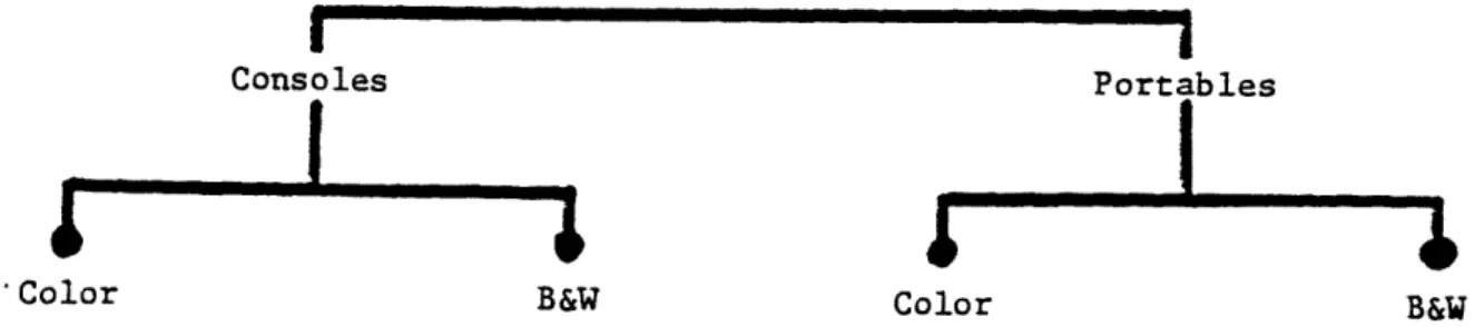
New product strategies also can influence and/or depend upon consumers' sequential decision processes. For example, consider market entry strategy. Selecting the "right" market to enter greatly enhances the likelihood and magnitude of a new product success. Selecting the wrong market can doom a new product to failure. One component of market selection is the identification of market structure such as the simplified hypothetical market structure for

televisions shown in figure 1. If, as shown, the consumer first chooses or can be influenced to choose among 'consoles' and 'portables' then among 'color' and

'black & white', a manufacturer of color consoles might favor color portables over black & white consoles so he can compete in both "markets" and not cannibalize his existing product line. Once such market structure is understood, the innovating

firm can better select a market on the basis of sales potential, penetration, scale, input, reward, risk, and match to the organization's capabilities (e.g., see Urban and Hauser 1980).

-2-I i

Consoles Portables

'Color B&W Color B&W

Figure : SimpZlified Hypothetical Hierarchy for TeLevision Markets

There are a myriad of other interesting, relevant situations where individual consumers are faced with sequential decision processes. In shopping behavior a consumer limits his set of product options by choosing one particular shopping center. The industrial salesman often tries to influence customer's consideration sets; supermarkets use displays to set one brand away from others; package goods manfactules often use similar packaging (compare Colgate to Close-Up toothpaste)

or distinct packaging; and some advertisements mention competitive products, others do not. Some of these strategies are planned, some dictated by

environmental constraints, and some serendipitous. But in each case the sequence of decisions among products is influenced and in each case the modification of the decision sequence may or may not affect choice outcomes.

We can better understand and model these marketing strategies if we first understand the effects of sequential processing on choice. By drawing on and extending recent developments in probabilistic choice theory, this paper explores a mathematical analysis of sequential decision processes, i.e., agendas, and their ability to influence consumers' probabilities of choice. We begin with a short discussion of research that addresses issues related to the issues we address in this paper.

In marketing, agendas have been studied by researchers seeking to influence market entry strategy with normative models that identify market structure. See review by Day, Shocker, and Srivastava (1980). Perhaps the best known example is

_-_-_-the Hendry system, described in Kalwani and Morrison (1977), which defines market structure relative to theoretical probabilities of switching among products. The identified agenda is based on a comparison of theoretical and observed switching probabilities. In a related method, Rao and Sabavala (1981) use hierarchical

cluster analysis on switching probabilities with the assumption that switching is greatest at the lowest levels in the hierarchy. Srivastava, Shocker, and Leone

(1981) apply a similar method to data which measures substitution-in-use. Urban, Johnson, and Hauser (1984) make the same switching assumption but use forced

switching data. They remove a consumer's most preferred product from a simulated store and observe subsequent behavior. In each of these methodologies, the

concern is a description of the market, not necessarily the individual consumer. In social choice economics, researchers have dealt primarily with voting agendas. Plott and Levine (1978) develop a descriptive model of "naive" voter behavior and illustrate that it fits empirical data quite well. McKelvey (1981) adapts this model to identify a "best" agenda via dynamic programming. In

alternative models, Farquharson (1969) and McKelvey and Niemi (1978) assume "sophisticated" voters who have perfect information about every other voters' preferences. These authors show that unique alternatives will be selected for binary agendas.

Our present approach differs from the approaches in these literatures. Unlike the social choice theorists, we deal with descriptive, probabilistic models of individual choice where the individual either is faced with a constrained agenda or uses an implicit agenda.

Unlike the market structure literature, we do not begin by defining agendas relative to the likelihood of switching among products. Rather, we investigate how such definitions and other properties are related to more primitive

assumptions of cognitive processing and its relationship to sequential and random decision structures.

Our purpose is to construct and investigate a mathematical representation, or theory, of how sequential cognitive decision rules affect individual choice

probabilities. We take as our basis, existing psychological models of choice behavior, models that have been used successfully (e.g., Tversky 1972 and Tversky and Sattath 1979) to describe and explain how individuals make choices among sets of choice objects. Because we are using these models in new ways, we need to make some generalizations, but we attempt to limit our generalizations so that our model clearly reduces to existing models when the choice situation is identical to that which has been studied previously. Furthermore, we do investigate a series of models which together bracket the types of hypotheses likely to be made about individual choice behavior.

We investigate and extend three decision rules: the constant ratio model (CRM), elimination by aspects (EBA), and the hierarchical elimination model

(HEM). We investigate their relationship to decision sequences and provide testable hypotheses as to when a decision rule would be used by an individual. Our analyses indicate when alternative decision rules provide different choice probabilities and when they do not, when and how agendas affect choice

probabilities, and how all of these results depend on the structure of interrelationships among choice objects.

Because we rely heavily on the recent literature in mathematical psychology, section 2 reviews the models we use in this paper. Section 3 defines an agenda and investigates its relationship to the choice probabilities. Section 4 explores the relationships among agendas and product attributes (aspects). Section 5

provides some illustrative results on when agendas are effective strategically. Section 6 discusses dominance and regularity and section 7 concludes with a discussion of limitations, extensions, and suggested experiments.

Throughout the text, we motivate the results with examples. All mathematical proofs are in the appendix.

5

2. PROBABILISTIC MODELS OF INDIVIDUAL CHOICE BEHAVIOR

Our review is by necessity concise. We seek to provide a basic review (1) because some readers may not be familiar with the details of these models, (2) our generalizations must be put in perspective, and (3) the remainder of this paper depends upon these models. Those readers wishing greater detail are referred to Luce (1959, 1977), Tversky (1972a, b) and particularly, Tversky and Sattath

(1979). Those readers already familiar with these models may wish to skip this section pausing only to review notation.

We use lower case English letters r, s, t, v, w, x, y, and z to denote choice objects, e.g., automobiles, restaurants, and televisions. We use upper case

English letters, A, B, C, ..., to denote sets of choice objects, e.g., A = x, y, z}. The total finite set of all choice objects being studied is denoted by T, and the null set is denoted by 0,

Let P(xjA) denote the probability that object x is chosen when the choice set is A. Naturally we assume P(xIA) > 0 and the sum of all P(xlA) for all x in A is equal to 1.0.

We describe choice objects as a collection of aspects. For example, an automobile may be described by aspects such as 'sporty', 'high mpg', 'sedan', 'front wheel drive', 'Chevrolet', etc. An aspect is a binary descriptor of a choice object, e.g., 'sedan', in the sense that a choice object either has an aspect or it does not. We use lower case Greek letters, a, X, y, ..., to denote aspects. For continuous attributes such as mpg, we define ranges. For example, an automobile with the attribute of 30 or more mpg, would have the aspect

'high mpg'. An aspect in this analysis can be a collection of more elementary aspects, e.g., 'high mpg, front wheel drive, sporty, and red', or it can be that which is unique to a choice object, e.g., 'Honda Accordness'.

Let x' = {a, 1,...} be the set of aspects associated with choice

alternative x. For any set of choice alternatives, A, let A' be the set of

-6-aspects that belong to at least one alternative in A; i.e., A' = {alax' for some tA) . For any aspect, a, and set of choice alternatives, A, let A denote the set of all choice alternatives in A that have aspect a, i.e., A = {xlxA, ax')}. Note that A' is a set of aspects and A is a

set of choice objects. For example, if A = {Honda Civic, Honda Accord, Chevrolet Chevette, Chevrolet Citation}, then A' = {'compact', 'front wheel drive', 'Honda', 'Chevrolet', ...}. If a = 'Honda', then A ({Honda

Civic, Honda Accord).

The best way to think of an aspect is as a unit of analysis. If attribute-like aspects, such as 'compact', 'front wheel drive', etc. are

sufficient to describe the choice process for strategic managerial understanding, then we prefer to work with them since they have intuitive appeal to the manager. However, it is not necessary that we be able to name the aspects. We can also think of aspects as descriptors of unique components of sets of choice objects. Aspects can be 'that which is unique to a Chevy Chevette', or 'that which is

shared by a Chevy Chevette and a Chevy Citation and no other car', etc. In such a specification, we could have an aspect for every possible subset of T, that is, 2n-2 aspects for objects. Both interpretations of aspects are consistent with our mathematical analysis. In fact, they would also be semantically equivalent if the manager could only articulate more elementary descriptors of

'that which is shared by a Chevy Chevette and a Chevy Citation and no other car'. Throughout the paper we use attribute-like aspects for our examples recognizing that our results apply equally well to the interpretation based on subsets of choice objects.

Constant Ratio ModeZ (CRM) . Perhaps the most commonly used probabilitic choice

model in marketing is the constant ratio model. See Bell, Keeney, Little (1975); Hauser and Urban (1977); Jeuland, Bass, Wright (1980); Johnson (1975); Luce (1959, 1977); McFadden (1980); Pessemier (1977); Punj and Staelin (1978); Silk and Urban

(1978); and others. The basic assumption underlying the CRM is that the ratio of (non-zero) choice probabilities for two objects is independent of the choice set. Mathematically, P(xJA)/P(ylA) = P(xjB)/P(yJB) for all A and B such that the

probabilities are non-zero. It is easily shown e.g., Luce (1977), that CRM implies there exist some scale values, u(x), for the objects, x, such that:

P(x[A) = u(x) (1)

Z u y)

yeA

where yeA denotes all objects, y, contained in choice set A. The simplicity of equation 1 has led to its wide acceptance. Furthermore, in many situations, it approximates behavior quite well. For example, Silk and Urban (1978) have forecast market share to within one or two percentage points on over 400 new products using a model that incorporates equation 1. See evidence in Urban and Katz (1983).

However, several authors (Debreu 1960; Luce and Suppes 1965; Restle 1961; Rumelhart and Greeno 1971; Tversky 1972b) have presented conceptual and empirical

evidence that CRM fails to account for the similarity among choice objects. For example, consider four automobiles, xl, x2, Yl, Y2 Assume xl and x2

are identical except for an unimportant aspect, say the type of electric clock, analog or digital, respectively. Automobile yl is quite different from x1 and

x2, but Y2 is the same as yl except for a very popular feature such as

cruise control. All four automobiles are priced identically. Suppose that an individual is indifferent between x1 and yl. Then, since xl and x2 are

virtually identical, we expect P(xll{xl, x2}) = 1/2, P(xll{xl, Y1}) = 1/2,

and P(x21{x2, y1 ) = 1/2, but P(y21{Yl y2 ) = 1. It follows from CRM (equation 1) tha

P(yl₁ {xl, x2, Y1}) = 1/3. However, common sense suggests the choice is more likely

among x-cars and y-cars. Consequently, we expect P(yll{xl, x2, Y1}) to be close to

1/2 and the other two trinary probabilities close to 1/4 rather than all equal to 1/3 as predicted by CRM.

-Furthermore, CRM implies if two automobiles are substitutable in one context they are substitutable in all contexts. Thus, if P(y21{yl,y2}) = 1,

then CRM implies P(y2J{xl,y2}) 1. Again, common sense suggests such a

result is implausible. The addition of cruise control is unlikely to eliminate all conflict among automobile x, say the Toyota Celica, and automobile y, say the Buick Skyhawk.

Elimination by Aspects (EBA). The above criticisms are formulated with

appeals to common sense based on similarities among the characteristics, or

aspects, of the choice objects. Elimination by aspects addresses these criticisms by postulating that choices among sets of objects depend upon the aspects of the objects not the objects per se. This assumption is analogous to the economic models of Lancaster (1971) and his colleagues and to the multiattributed models in marketing as reviewed by Wilkie and Pessemier (1973).

EBA postulates that an individual chooses among all aspects in the offered set, A', with probability proportional to the scale value of the aspect. He then eliminates all choice objects not having the chosen aspect and continues choosing

aspects and eliminating objects until one choice object is left. If a represents the scale value of aspect a, then EBA is given mathematically by the following recursive equation:

P(xIA) =

a

. P(xjA ) (2)

Bx3A'

It is easy to show that any aspect common to all alternatives in a choice set, e.g., the aspect 'automobiles', does not affect choice probabilities and will, therefore, be discarded. See Tversky (1972a, 1972b).

To illustrate EBA, we consider four automobiles x = Honda Civic, y = Honda Accord, z = Chevrolet Chevette, and w = Chevrolet Citation. Let a = 'Automobile',

3 = 'Japanese', y = 'American', 6 = aspects unique to the Honda Civic, = aspects unique to the Honda Accord, X = aspects unique to the Chevrolet Chevette, and

n = aspects unique to the Chevrolet Citation. According to our definitions:

---X' = {a(, a, }

y' {a, 3,}

z' = , X}

w' = {a, Y, n}

The aspect, a, is common to all objects and can be ignored. Alternative x will then be chosen if is the first aspect chosen or if is the first aspect chosen and then 6 is chosen from the set ({, p}. Specifically:

P(xlix, y, , w}) = 6 + . P(xl{x, y}) (3)

=6+, .

6

d +R

where, without loss of generality, we have set

$+

+ + / + + = 1. To illustrate how EBA resolves the conceptual criticisms of CRM, set a = unique aspects of Toyota Celica, = unique aspects of Buick Skyhawk,

Y1 = digital clock, y₂ = analog clock, and 6 = cruise control. Then,

xY' = { y1}

x'

=

{a,

Y 2}

Y1 {

y2 2(, 6}

Y2 fat

Suppose

a

= , Y1 = Y2, and Y1, Y2, and are small compared to cc and B.

Then equation 2 yields: P(yll {x l, x₂' Y₁}) ) = /( + o + y + 2) /(a + ₎

= 1/2. Similarly, P(y21{xl, y2}) = (+5)/(f++a+yl1) = /(Ct+f) = 1/2.

We leave it to the reader to show that all other binary and trinary probabilities are as expected by common sense.

EBA is a generalization of CRM because equation 2 reduces to equation 1, with u(x) = x, , when choice objects are disjoint, i.e., x'fy' = 0 for all

x, yeA.

Finally, note that EBA does not imply a fixed sequential decision process. Rather, EBA implies that the individual probabilistically selects aspects for

consideration and, hence, EBA is a randomized sequential decision process.

- 10

Preference Trees

By 1985 there were over 160 different automobiles available. The number of aspects necessary to fully describe and distinguish these automobiles could be very large. For example, if there were an aspect for every possible subset, a fully specified EBA model would require approximately 1.5 x 1048 aspects. At the other extreme is CRM, which applies when objects have no shared aspects. CRM requires only as many scale values as there are choice objects, in this case 160 scale values.

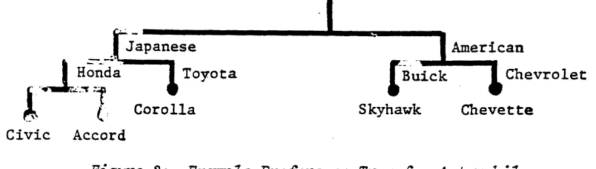
Tversky and Sattath (1979) investigate an intermediate level of complexity in the structure of aspect sets. They investigate tree structures known as

preference trees. An example preference tree is shown in figure 2.

L

:an

Chevrolet .tte Civic Accord

Figure 2: Example Preference Tree for AutomobiZes

A preference tree is an aspect structure which is a hierarchical aspect

structure where there is no overlap among the branches. For example, in figure 2 there are Japanese and American automobiles. The Japanese cars are further

subdivided into Hondas and Toyotas and the American cars are subdivided into

Buicks and Chevrolets. The addition of an American Honda say if consumers considered Hondas built in America as American, would introduce overlap and upset the tree

structure. (See formal definition of preference trees in Tversky and Sattath 1979). A preference tree structure greatly restricts the complexity of the inter-relationships among aspects. The 2 -2 possible aspects are limited to at most 2n-2 aspects corresponding to the maximal number of links in a tree with n

- 11

terminal nodes. For example, in a choice set with 10 objects, the number of

aspects possible are reduced from 1,022 to 138. Thus, preference trees represent a compromise between the generality of unrestricted EBA and the limitations of CM. Nonetheless, preference trees can adequately represent many interesting choice situations. For example, the structured choice set, {xl, x2, y1 Y2} ,

shown above is the preference tree in figure 3. (The vertical length of the branch indicates the importance of the feature.)

Celica (a) Skyhawk ()

I,

,b1.--- --- \, ''1 *Analog

clock (y2)

xl1 2 Y1 Cruise control ()

Y2

Figure 3: Preference Tree Representation of the Logical Counterexample to the Constant Ratio ModeZ.

HierarchicalZ EZimination ModeZs (HEM)

Neither CRM nor FBA are sequential decision rules. Preference trees are aspect structures, not decision rules. However, there is empirical evidence that individuals make explicit, hierarchical decisions. See among others Bettman (1979), Haines (1974), and Payne (1976).

In 1979, Tversky and Sattath introduced the hierarchical elimination model (HEM) to represent cognitive processing on a preference tree as a hierarchical series of choice points. The idea is that the individual sequentially compares

sets of objects defined by branches in the preference tree. For example, in

figure 2 he first decides among 'Japanese' and 'American' automobiles, then, if he selects 'Japanese', he chooses among 'Hondas' and 'Toyotas', and finally, if he selects 'Hondas', he chooses among 'Civics' and 'Accords'. The choice among branches is proportional to the measures of the aspects in that branch. For example, if a = 'Japanese', 3 - 'American'. y = 'Honda', 6 = 'Toyota',

12 -'niait-n rnrk ( i

- ''Buick', X = 'Chevrolet', = 'Civic', and = 'Accord', then the probability he chooses the 'Japanese' branch is:

P(JapaneselT) = (a+ Y+ 6 + + (4a)

(a

+ y

+

6 +

+7)

+

(+P

+X)

The probability he then chooses the Honda subbranch is:

P('Honda'I'Japanese') Y +

4

+ 7 (4b)

(Y+

+ 7)

+d

and

P('Civic'j'Honda') = (4c)

The overall probability is the product of the sequential conditional probabilities, i.e.,

P('Civic'IT) = P('Civic'I'Honda')P('Honda'j'Japanese')P('Japanese'IT) (4d) In other words, if Al, A₂, ... , T is a sequence of choice sets such

that Ai is contained in Ai+l and if the sequence corresponds to-the branching in the preference tree, then a hierarchical probability model is given by:

P(xA) = P(xIA1)P(AlA 2) *.. P(A,_lAlI)P(AI T ) (5)

where A denotes the hierarchy.

For a preference tree, HEM is defined such that

P(xAl) = m(x) (6a) C m(y) ye A₁ P(AilAi+ ) m(Ai) (6b) i m(B) BcAi+1

where m(Ai) denotes the measure of A and BAi+1 indicates the sum is over

all branches B of the set Ai+₁. The measure of Ai is equal to the sum of all aspects in Ai except those shared by all other branches in A i+l The measure of x is the sum of all aspects of x except those shared by all objects in A. For example, in figure 2 and equation 4, m('Civic') =

4,

m('Accord') = 7,

m('Honda') = Y + +

77,

m('Toyota') = 6, etc.

13

To see how HEM resolves the conceptual criticisms of CRM, we apply HEM to the preference tree in figure 3. Using equations 5 and 6 and the definitions of ,

, Y1' and Y2 for that figure, we obtain:

P(ylj{xl, x

₂

,

Y

1

})=

/(a+f+Y

1

+Y

2

)

/

=

1/2

Pi{X1X· X2,

·Y1

)=

1+y

.

Y1

r1

+Y 2+ / \ Y2Y1+

Clearly, HEM and EBA are very different cognitive decision rules.

Intuitively, we would not expect them to yield the same choice probabilities. However, the reader may wish to verify that for the preference tree in figure 3, the forecast choice probabilities are the same for EBA and HEM. Tversky and

Sattath (1979, p. 548) prove the surprising result that for any preference tree, EBA and HEM yield the same choice probabilities. Thus, on a preference tree, we

could never distinguish the two alternative decision rules by simply observing choice probabilities. (However, we might distinguish them by other means such as verbal protocols or choice reaction time.) V

To date, HEM has only bn defined for preference trees. The preference tree defines a natural sequence of decisions. We now extend the preference

tree/hierarchical elimination concepts to general aspect structures, general sequential decisions and to imposed sequential constraints on choice decisions.

3. AGENDAS

If the aspect structure forms a preference tree and the consumer follows HEM, then we can think of the choice process as following a sequence of constraints. That is, the consumer first chooses a set, i, from among subsets of T, next he (or she) chooses a set, A ' ₁ from among the subsets of A,

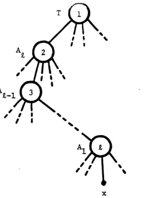
proceeding until he (or she) finally chooses an object, x, from the choice set Al. The choice sequence is illustrated in figure 4 where the nodes represent choices. We have numbered the nodes to indicate the order of processing in HEM. In HEM the sequence is defined by the natural structure of the aspect tree.

-T I I AZ-₁ 4f , r I

Figure 4: Schematic Representation of Sequential Choice Process in IHEM

on a Preference Tree.

There are, however, many situations in which the aspect structure is not a preference tree and/or the sequence of decisions are not determined by the

aspects. For example, the aspect structure in figu-re 1 is noi a pcference tree because the aspects, 'color' and 'B & W' appear on both the 'consoles' branch and the 'portables' branch. In fact, figure 1 is more like a factoLial structure than a tree structure. We expect such factorial structures to be common in mature markets like television sets where the market has evolved such that competitors

have exploited all segments.

Even if the aspect structure is a tree, there may be external constraints which force a sequential process that does not follow the tree. Consider the

faculty candidate who is constrained to a geographic area because of a spouse's opportunities or the automobile owner who is constrained in a choice of service

stations because the automobile requires diesel fuel.

Even if no constraints are imposed, a consumer may wish to make choices sequentially. Consider restaurant choice in an unfamiliar city. We often

simplify our decisions by first choosing price range, say high, medium, or cheap eats, and then style, say French, Italian, German, American, Chinese, Israeli, or Lithuanian. Such a choice process can be viewed as a set of (internally imposed)

constraints.

- 15 -I

We define an agenda as a sequence of constraints. In particular, an agenda is a tree of objects such that at any node, say A in figure 4, the consumer must choose among those branches exiting that node. We label the nodes to indicate the order in which they are processed. For example, in figure 4, the agenda is

processed from the top down as indicated.

However, an agenda need not be top down. It can also be bottom up as shown in figure 5.

Peking Garden Yantze River Cory's Friendly's Versailles Bel Canto

Figure 5: Bottom Up Agenda for Restaurant Choices in Lexington, MA.

In figure 5, we first choose the best restaurant in each class, say Yantze River for Chinese, Cory's for American, and Versailles for other. We then choose the

restaurant for a night out by comparing the best with the best, in this case, Yantze River vs. Cory's vs. Versailles. Such an agenda might be used by a

resident of Lexington, MA who is familiar with all six restaurants. On the other hand, a tourist unfamiliar with Lexington, may process this tree with a top down agenda. Notice that the processing sequence is a logical constraint not

necessarily a temporal constraint in the sense that all '1' nodes do not need to be processed simultaneously. We only require that all '1' nodes be processed prior to any '2' nodes.

We also allow agendas to be mixed. For example, a consumer may process all bottom nodes, then the top node, and finally the intermediate nodes.

-

16

-III

We denote agendas by upper case script letters, A, B, C, ..., and represent

them by labeled diagrams such as figures 4 and 5. For top down agendas we use a superscripted star, i.e., A*, and for bottom up agendas we use a subscripted star, i.e., A*,. When an agenda is either all top down or all bottom up we can represent the agenda more simply by nested sets. For example, {{x, y}, {v, w}

indicates we first choose among {x, y} and {v, and then within either { x, y} or {v, w}. Alternatively, {{x, y}, {v, w},* indicates we first choose

among x or y and among v or w, and then compare the best with the best, say x with v.

Relationships to Choice ProbabiZities.

We illustrate first the relationship of EBA and HEM to top down agendas. Next, we illustrate the. effect of bottom up agendas and then we investigate which choice

rules are affected by agendas.

Eimintion--Aspects (EBA) and Agendas. Suppose that a onsumer uses EBA

whenever he is presented with a set of choice objects, but we constrain him to follow an agenda from the top down. For example suppose that T is partitioned into A and B and we force the consumer to choose first among A and B and then within A

or B. Following Tversky and Sattath (1979) we assume that the probability of choosing A from T equals the sum of the probabilities of choosing any object in A

from T. In our example, such a combination of constraints and EBA says simply:

P(xIA) - P(xlA)P(AIT) (7)

where P(xjA) P(ylT)

and P(xJA) and P(ylT) are given by EBA. (We can clearly generalize equation 7 to more than one intermediate level. For example, see equation 5.)

To see that such constraints can affect choice probabilities, let T {x, y, v, }

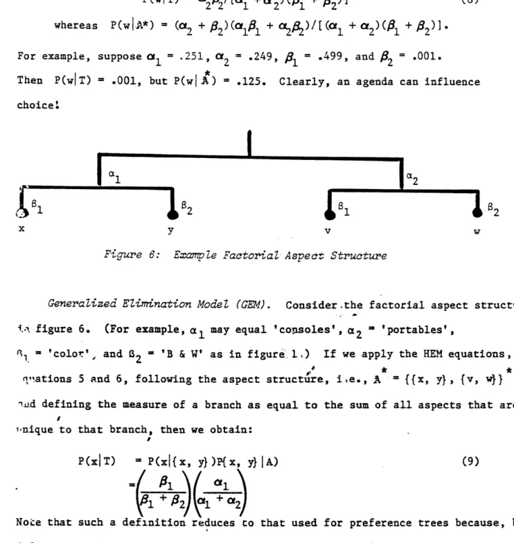
let A = {{x, w}, {y, i} , and let the aspect structure be given by figure 6. That is, x' = {a, 1} Y' ' (al I2}, v' ' {a2i, B1' and w' ({a2, 2

Notice that T is a 2 x 2 factorial structure. Then, after some algebra:

17

-ll____al_·_CI__el__Y____

___________1111__1__111_____11_1___

-III

P(wlT) = [al 12-2/ + 2) (1 + 2) (8)

whereas P(wl.A*) = (2 + ₂)(aOIl + 4 )/ (a* l a₂+ )(2)

For example, suppose al = .251, a2 = 249, 1 = .499, and 2 = .001.

Then P(wlT) = .001, but P(wl A) = .125. Clearly, an agenda can influence choice

x y v w

Figure 6: ExampZe Factorial Aspect Structure

Generalized EZimination ModeZ (GEM). Consider.the factorial aspect structure

i.. figure 6. (For example, al may equal 'consoles', a₂ = 'portables',

l. = 'color', and ₂ 'B & W' as in figure 1,) If we apply the HEM equations,

n,uations 5 and 6, following the aspect structure, i e., A = {{x, y}, {v, } , Aiud defining the measure of a branch as equal to the sum of all aspects that are ,nique to that branch, then we obtain:

P(xlT) = P(x{x, y})P{x, y}IA) (9)

=(

_ 0l

NoCe that such a definition reduces o that used for preference trees because, by definition, there are no aspects shared among branches of a preference tree.

We define a more general model, GEM, by equations 5 and 6, but we allow the measure of a branch to be a general function of the unique and shared aspects of a branch. The above definition is but one example where the shared aspects, in this case, ₁ and B2, have no effect on the probability of choosing a branch.

18

To illustrate that the choice of how one computes the measure of a branch can have an impact on choice probabilities, consider the aspect structure in figure 6 and the top down agenda, = {{x, y}, v} . Suppose

a

1

=.03,

a

2 = .07

P1

=.80, and 82 =.10. Apply GEM with no consideration of shared aspects when computing m({ x, y}) would imply:

P({x,

y}UB*)

=

al

+

82

(10)

( 1

+

82) +

a

2

P({x, y} I ) > P({x, y} A ) as expected by the axiom of regularity and 82 enters the calculation, but intuitively we would not expect the deletion of w to raise P(xB*) from .3 to .6 as equations 9 and 10 suggest. More likely, we would

expect that 1, which can be obtained on both branches, would also affect P({x, y}B 3).

Perhaps we should consider shared aspects in computing branching prob-abilities. For example, we might compute P({x, y}lB ) by including 81

thus:

P({x, ylj*)= 18+ ()

(

+ 2 + l) + '

e

l)

where we have weighted the measure of ₁ by a scale factor of

e

in the range

0 < < 1. If

8

= 0, equation 11 reduces to equation 10. However, if = 1

using the scale above, we obtain P({x,y}[ 3*) = .46 and P(x3B*) = .4, which is a more reasonable increase in the probability of choosing x.

It is an empirical question as to how shared aspects affect branching probabilities. Since equation 11 reduces to HEM on a preference tree for any value of , we define HEM( ) as a special case of GEM when the measure of a branch equals the sum of all unique aspects plus

e

times the sum of all shared aspects. In section 5, we investigate the strategic implications of shared aspects, that is, of .

- 19

I1___II___I___III_1_^-1---^1·-^--Bottom Up Agendas. In a bottom up agenda, we represent a choice set by its

best choice object, a processing rule often advocated by economists. Processing proceeds much as an athletic team proceeds through a tournament. In particular,

for the aspect structure in figure 6 and the agenda, A = {{x, y}, {v, }*,

we compute equation 12 if the consumer uses EBA for any unconstrained choice.

P(x1A*) = P(x{x, y} )[P(xl{x, v} )P(vl{v, ) + P(xl{x, w}) P(wl{v, )] (12)

=(

11

\

al

\

1

\+

(

+ 1

2

1

+1

2

/[

1

+a2

1

+

2

l +

1 +a2

+

2 1+2

Using

a(

= .051,

a

2 = .049, 1 = .64, and 82 = .26, we obtain P(xA*) = .40

compared to P(x[T) = .36 which we would obtain via unconstrained choice. In this case we see that a bottom up agenda enhances slightly the probability that the "best" choice object, x, is selected. (x' = {al, 1} and al > a2 1 > 82'

hence, we call x "best",) We will see in section 5 that, in general, certain bottom up agendas enhance "good" objects while making "bad" objects less likely to be chosen.

For now, suffice it to say that bottom up agendas do affect choice and do so

differently than top down agendas. For example, with EBA on the above aspect measures, P(xIA*) = .36, which turns out to be the same as the unconstrained choice, P(xlT).

Invariance. We have already shown many examples where agendas affect choice

probabilities. We might wonder whether agendas always affect choice probabilities or whether there is any choice rule for which choice probabilities are not

affected by agendas. We call such unaffected choice rules invariant.

Consider the factorial aspect structure in figure 6. The example in equation 8 has shown that the agenda, A = {{x, w}, {y, v}}* affects EBA choice

probabilities. Similarly, if we compute HEM(O) for A , we obtain:

P(wIA*) = 1/2 ( t2 + 2 (16)

l+ a2 + f + 2

20

which is clearly different than the expression for P(wjT) obtained in equation 8. This example illustrates that, in general, neither EBA nor HEM (0) are invariant with respect to top down agendas.

It is easy to see that for top down agendas, a cognitive processing model is invariant if and only if P(xlT) = P(xfA)P(AIT) for any A whenever A is a subset of T and P(xlT) is non-zero. However, this condition is Luce's (1959) choice axiom which is the defining property of CRM. Thus, for top down agendas, CRM is the

only invariant decision model.

Consider the bottom up agenda, ,

-

{{x, y}, {v, w*. Applying CRM to each pair gives us:

P( l)

u(x)

\.r/v)

+

U(x)

U(w)

V u(+ U(v u(V (w Vx+ x u(w) u(v) + w which does not reduce to CRM model of

P(xlT) ' U(x)

u(x) + u(y) + u(v) + u(w)

Thus, not even CRM is invariant with respel- to bottom up agendas. Since EBA and HEM( i) are equivalent to CRM when there is no overlap among the aspect sets of x, y, v, and w, this example is sufficient to show that CRM, EBA, and HEM ()

can be affected by bottom up agendas. To date, we know of no decision rules which are invariant with respect to bottom up agendas.

We state this result as a theorem since it is important conceptually even if it is easy to prove mathematically.

Theorem Z (Invariance): The constant ratio model is the only decision rule invariant with respect to top down agendas. On the other hand, each of the decision rules, CM, EBA, and HEM(e) can be affected by bottom up agendas.

Theorem 1 is encouraging. Agendas do affect choice. We should be able to identify at least some agendas that affect choice in scientifically interesting and managerially useful ways.

21 -

I^--Theorem 1 has an additional benefit because it provides a means to test

whether CRM is a reasonable descriptive model of behavior. That is, if no top down agendas can be found to affect choice, then CRM is not eliminated as a decision rule. If any top down agenda affects choice, then CRM cannot be the decision rule.

Behavioral Hypotheses - FamiZiarity

The preceding analysis introduced agenda constraints and illustrated their effect on choice probabilities. In some cases the constraints will be imposed externally, but in other cases, they will be the result of self-imposed

simplifications in cognitive processing. We close this section by setting forth initial hypotheses as to when self-imposed agendas are likely to be used by

consumers. These hypotheses are empirically testable. While our analytic results in subsequent sections do not depend explicitly on the validity of these

hypotheses, these hypotheses do serve to motivate and interpret self-imposed agendas.

Top Down vs. Bottom Up Agendas. In figure 5 we illustrated bottom up agendas

with restaurant choice. Suppose you are a a conference in an unfamiliar city, say San Francisco, and you are faced with a restaurant choice. You have not experienced the various restaurants, but you have some idea as to what to expect. You may first decide on a seafood restaurant because San Francisco is known for seafood, then decide on one near your hotel, ask or read about nearby seafood restaurants and make a choice. When you arrive at the restaurant you select an item from the menu. This is clearly a top down hierarchical choice process.

Suppose instead you are at home and are faced with a restaurant choice. Since you eat out often, you know what you are likely to order at each restaurant, i.e., the restaurant is represented by its "best" item according to your tastes and taking prices into account. You compare these "best" items when selecting the "best" seafood restaurant, and you compare the "best" seafood restaurant to the

-"best" Chinese reseaurant to the -"best" Italian restaurant, etc. when making your final choice. This is a bottom up hierarchical choice process.

Consider the hiring decision in the introduction to this paper. If there are many candidates and the search cost is high, we would likely narrow the field by

deciding on an area of interest. On the other hand, if search cost is low as in the case of few candidates, we might use a bottom up, "best" versus "best"

decision rule.

Similarly, if we are hiring at the "junior" level, we may be more likely to use a top down decision process because we are uncertain, even after a campus

interview, how productive the candidate will be. At the 'senior' level we have much better information on research and teaching productivity and may be more

likely to use a bottom up process where we compare, say, the best available model builder with the best available consumer behavioralist.

In each of these anecdotes, the key variable is familiarity. In general, we posit that:

When one is very familiar with objects or search cost is low, and

uncertainty is low, then a bottom up agenda will be favored. When one is unfamiliar with the choice objects, and search cost is high, or

uncertainty is high, then a top down agenda will be favored. One implication of the above familiarity hypothesis is that lack of information will lead an individual to a top down choice process and could conceivably lead him to eliminate an optimal choice object early in the

hierarchy. For example, suppose the "best" Seattle restaurant is not a seafood restaurant or the "best" junior faculty candidate is not in the area we choose.

EBA vs. GEM. GEM computes representative measures to summarize the attractiveness of a branch. Constrained EBA sums the probabilities of the

individual items. As with top down agendas, we expect representative measures to be used more often when detailed information about the objects is unknown,

uncertain, or difficult to obtain. We posit that:

23

--III

For constrained top down agendas, GEM will be the operant rule when detailed information is not available, while EBA will be favored when detailed information is available.

In analyzing the familiarity hypothesis, it is important to recognize that both GEM and EBA are paramorphic models of cognitive processing. GEM does not necessarily imply that an individual uses the postulated arithmetic rule to compute the measures, m(y), of each branch, but rather that the arithmetic

rule will provide a good estimate of the weight he (or she) will attach to each branch. Thus, according to the familiarity hypothesis, an individual will assign weights

to branches based on limited familiarity. These weights will be similar to what we, as analysts, compute by the GEM rules.

4. ASPECT STRUCTURES AND AGENDAS

We have already considered special aspect structures in the form of preference trees such as the automobile example in figure 2. There is another class of

aspect structures that is important and which is also more parsimonious than a general structure.

Consider controlled experiments where the researcher manipulates the choice objects, product categories where features dominate unique brand images, and

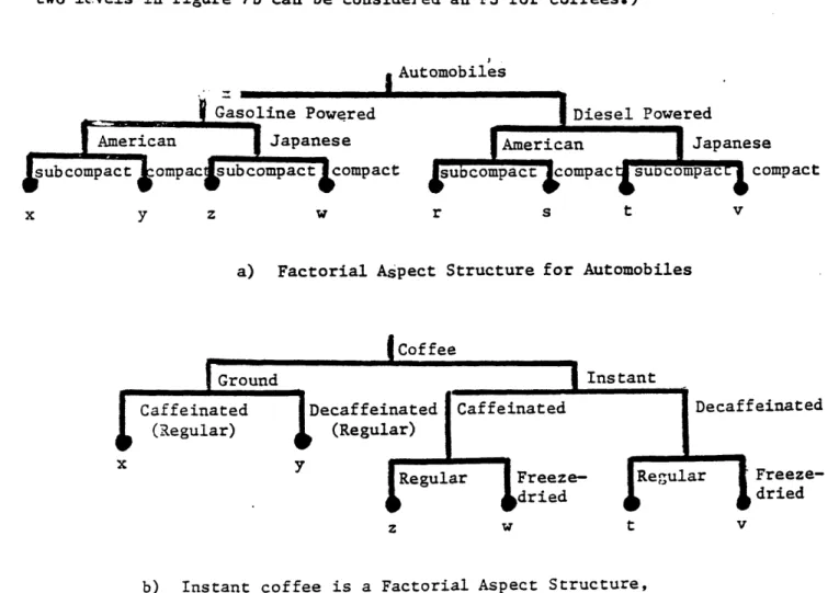
product categories where manufacturers have exploited market segmentation by offering all possible combinations of features. In each of these instances we might expect to see factorial structures. For example, figure 7a is a factorial structure which represents an alternative hypothesis about the automobile market. In a factorial structure there is overlap among branches and that overlap is complete in the sense that aspects are partitioned into groups such that each object has exactly one aspect from each group and all possible combinations of these aspects are represented in the choice set.

-Factorial structures (FS) occur often in marketing. For example,

applications of conjoint analysis in marketing rely heavily on factorial designs (possibly fractional) for data collection. See review by Green and Srinivasan (1979). Similarly, factorial experimental designs are used to investigate consumer behavior theories. See Sternthal and Craig (1981). Some markets

naturally evolve as factorial designs as line extensions are introduced to fill every market niche.

For example, one might describe instant coffees as 'caffeinated' versus 'decaffeinated' at one level, and 'regular' versus 'freeze dried' at another level. See empirical evidence in Urban, Johnson and Hauser (1984). However, as figure 7b illustrates, the entire coffee market may not be a factorial structure because there are no freeze-dried ground coffees. (On the other hand, the first two levels in figure 7b can be considered an FS for coffees.)

A..e hmrh; 1 bec

!se compact

y z w r s t v

a) Factorial Aspect Structure for Automobiles

'einated

Freeze-dried

z w t v

b) Instant coffee is a Factorial Aspect Structure, but coffee is not.

Figure 7: Aspect Structures

IN c

X

---At this point it is worth digressing to recognize that the definition of aspects may be only an approximation. For example, in the instant coffee market there may be other differences between brands than those shown in figure 7b. Taster's Choice may have a different color label than Folaer's and that

color may matter in consumer choice. By analyzing the instant coffee market as an FS we are assuming that the specified features (aspects) dominate the features we do not model explicitly. The validity of such assumptions can only be answered empirically, but such assumptions do allow us to isolate and study agenda effects recognizing that, in application, we might have to include other effects in our

analysis.

ConmpatibiZity

Theorem 1 shows that only CRM is unaffected by all top down agendas. But, this does not mean that all agendas affect choice outcomes. For example, it is clear that an agenda that matches, or at least does not disrupt, a GEM hierarchy will. .t affect GEM choice probabilities. But how about EBA? EBA is not a

hie: .chical. processing rule but is instead a random access processing rule. Inti.;:ily, we expect agendas to influence EBA probabilities.

But not all agendas do affect EBA probabilities. Consider the factorial structure in figure 6 and the "compatible" top down agenda structure in figure 8. First we compute an unconstrained EBA probability.

P(xIT) 1l 81 + 1 1 (13)

\l1 82 plcl2/ 1 + a2/ 1 + +2/

x y v w

ifure 8: 4aenda Structure "ComratibZe" with FactoriaZ Aspect Structure in Figure 6.

- 26

where we have assumed t₁ + 1a₂ + 1 + 2 = 1 without loss of generality. Now we compute the EBA probability constrained by the agenda in figure 8.

P(xlA*) = P(x{x, y})P({x, y} T)

_ 1 +l +1 + \ 2

01al (l / i ) (14)

+ 21 \ + 2

They are the same: As it turns out, this result generalizes.

Following Tversky and Sattath (1979), we call two trees compatible if and only if there exists a third tree, defined on the same choice objects that is a

refinement of both. For example, {{{x, y}, z}, {t, v, w}} and {{x, y, z}, {{t, v}, w}

are compatible since {{{x, y}, z}, {{t, v}, w}} refines both agendas. On the other hand, {{x, w}, {y, v}} is not compatible with {{x, y}, {v, wI}

since there is no tree which refines both these agendas. Note that the degenerate tree {x, y, v, w, ... }, implied by CRM is compatible with all trees on T. For

factorial structures, an agenda is compatible if each branch of the agenda corresponds to dividing the factorial structure on the (factorial) groups of aspects.

Tversky and Sattath (1979) have shown that, in general, constrained top down agendas do not affect choice probabilities if the aspect structure is a preference tree and the agenda is compatible with the preference tree. We show in the

appendix that this result also holds if the aspect structure is a factorial structure and the agenda is compatible with the factorial structure.

We also show the more surprising result that compatible preference trees and compatible factorial structures are the only agendas that do not affect choice probabilities. Except for specific choices of aspect measures1, all

We can always find degenerate cases in which P(xJT) = P(xlA*) for some choice of aspect measures. For compatible pretrees and FS's and only for compatible pretrees and FS's, P(xJT) = P(xlA*) for all choices of non-zero

aspect measures. Define compatibility for non-tree/non-factorial when, for each split due to the agenda, there is a set of aspects contained in each branch that are contained in no other branch in the split.

other agendas will affect EBA choice probabilities. Even fractional factorial agendas and incomplete factorial agendas similar to figure 7b will affect choice. Formally,

Theorem 2 (Compatibiiitv): For an arbitrariZy chosen set of aspect measures, a constrained top down agenda, A*, has no effect

on a family of EBA choice probabilities, P(xjT) for allZZ xeT, if

and only if either (Z) the aspect structure forms a preference tree and A* is compatible with the tree or (2) the aspect structure forms a factorial structure and A* is compatible with the factorial structure.

The detailed proof to theorem 2 is long and complex. Basically, we first show that EBA is algebraically equivalent to a hierarchical rule for preference trees and

factorial structures and only for preference trees and factorial structures. We then show that a compatible agenda does not upset the hierarchical nature of the

calculation.

Theorem 2 is both interesting and uiseful. Consider the television example in figure 1, which is a factorial strr.1;:,c_ r ih aspects 'consoles' versus

'portables' and 'color' versus 'B & , Fo£ ?,BA, theorem 2 implies that an

advertising campaign will have no a f t~ it attempts to influence consumers to make decisons according to the hiel'ah d !i figure 1. Nor will a 'coior' versus

'B & W' campaign have an effect. Ho.-ever, a campaign encouraging the comparison 'color portables' to 'B & W consoles' will affect choice probabilities. Theorem 2 also cautions behavioral researchers o avoid agenda experiments on compatible factorial structures if they wish to denfity agenda effects from observed behavior.

To date, we know of no aspect structures which are not affected by bottom up-agendas.

Equivalence

Compare the calculation of P(xI' ) via HEM(O) in equation 9 to the

calculation of P(x T) via EBA in equation 13. Although the procedure by which we calculate the choice probability differs dramatically, we obtain the same answer.

This is true despite the fact that HEM and EBA are quite different

-hypotheses about how a consumer processes information to make a choice. For example, HEM is an explicit, sequential, top down decision process while EBA is a random access elimination process.

The calculation in equations 9 and 13 were based on the factorial structure in figure 5. It turns out that this result generalizes to all factorial structures and, as shown earlier by Tversky and Sattath (1979), to preference trees. But the result holds for no other structure.2 Furthermore, the result does not hold

when shared aspects are considered, i.e., when

e

is not zero. Formally,

Theorem 3 (Eauivalence): For an arbitrarily chosen set of aspect

measures, the generalized hierarchial elimination model and eim-inavion by aspects yield equivalent choice probabilities if and only if (Z) the aspect structure is a preference tree or (2) the aspect

structure is a factorial structure, 9=0, and the hierarchy associated

with HEM is compatible with the preference tree or factorial structure.

An immediate corollary of Theorem 3 is that HEM(Q) probabilities are

independent of the order in which aspect partitions are processed. (For-

e

o,

the order can be shown to matter.) Thus, if a researcher uses a factorial

structure experiment to investigate hierarchies and the subject(s) is using HEM(O) or EBA, the researcher will not be able to identify the order of aspect processing or the decision rule the subject is using by simply observing the choice

outcomes. However, the researcher may be able to identify orderings or decision rules by other means such as verbal protocols or response time.

Furthermore, in a market that has evolved fully to a factorial structure, say some automobile submarkets or the instant coffee market, managerial actions to influence agendas will not depend upon the specific cognitive processing hierarchy as long as EBA or a compatible HEM(O) applies.

2

Except, of course, for specific choices of aspect measures. We seek the result that holds for arbitrarily chosen aspect measures.

-III

Swaary

Theorems 2 and 3 illustrate the very special nature of preference trees and factorial structures. For such aspect structures and only for such aspect structures, compatible agendas do not affect EBA probabilities and these EBA probabilities are equivalent to hierarchical elimination probabilities. Theorems 2 and 3 do suggest that other agendas will affect choice

probabilities.

We turn now to an analysis of which agendas do affect choice probabilities.

5. STRATEGIC IMPLICATIONS ON FACTORIAL STRUCTURES

In general, agendas affect choice, but section 4 suggests that the effect depends upon the type of agenda, the aspect structure, the decision rule, and the measures of the aspects. To a marketing manager seeking to improve the probability that his (or her) product is chosen, these are very important questions. For

example, if the manager wants to design an advertising campaign to influence

consumer agendas, that is, to influence to which competitive products his roduct is compared, he (or she) will want to evaluate the likely directional effect of his (her) campaign. If the directional effect depends only upon the aspect structure, not

upon the specific measures of the aspects, so much the better,

In this section we illustrate the strategic implications of agendas on 2 x 2 factorial structures. Such factorial structures serve to illuminate more general results, but are sufficiently easy to visualize so as to not obscure the intuitive understanding of agenda effects.

We begin with dissimilar groupings, a class of top down agendas that enhance a lesser target object. We then illustrate bottom up agendas which enhance greater objects. Finally, we explore the comparative implications EBA and HEM and the effects due to shared aspects. Throughout this development, we assume the

-factorial aspect structure in figure 6, that is, x' {a l 1}, Y' = {al,' 2}

v'

=

{a

₂

' 31

} '

and w' = {a

₂

' 2}'

Enhancement of a Lesser Object

Marketing folk wisdom suggests that perhaps it is always effective for a low market share product to force a comparison between itself and a high market share product. For example, there are many advertisements in which a 'cola' is compared to Coca-Cola. A similar phenomenon appears to be true for the Pitney Bowes/

Savin/Xerox example. However, many automobile manufacturers go out of their way to compare themselves to the low share, but prestige, products of BMW and Mercedes.

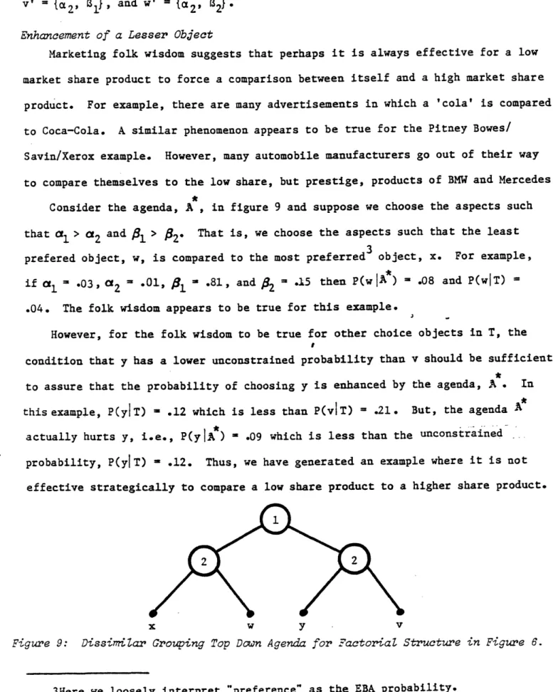
Consider the agenda, A , in figure 9 and suppose we choose the aspects such that

al

>

a

2 and f1 > ' 2 That is, we choose the aspects such that the least

prefered object, w, is compared to the most preferred3 object, x. For example, if

a

₁ = .03,

a

2 = .01, 1 = .81, and 82 .15 then P(w A) .08 and P(wIT) = .04. The folk wisdom appears to be true for this example.

However, for the folk wisdom to be true for other choice objects in T, the condition that y has a lower unconstrained probability than v should be sufficient to assure that the probability of choosing y is enhanced by the agenda, A . In this example, P(yTT) - .12 which is less than P(vIT) = .21. But, the agenda A

actually hurts y, i.e., P(y]A*) .09 which is less than the unconstrained probability, P(ylT) .12. Thus, we have generated an example where it is not effective strategically to compare a low share product to a higher share product.

x w y v

Figure 9: Dissimiar Grouping Top Down Agenda for Factorial Structure in Figure 6.

3Here we loosely interpret "preference" as the EBA probability.

31

Fortunately, we can identify an interpretable condition where an agenda is effective independent of the specific aspect measures. In particular, if we group the object, w, in a top down agenda with that object, x, for which w is maximally

dissimilar but inferior, then the agenda will enhance the probability that w will be chosen. This result holds independent of the specific aspect measures as long as a₁ > 2 and

,1

> 82' We state the result for a 2 x 2 factorial

structure, but in the appendix we show it generalizes for an Q-level factorial and for more aspects.

Result (Dissimilar Grouping): For the factorial structure in

Figure 6, the top down agenda, A* = {{x, w},{y,v}}*, enhances the

EBA probability that the least referred object, w, is chosen and hurts the EBA probability that the most preferred object, x, is chosen.

That is, P(wIA*) > P(wIT) and P(xIT) > P(xIA*).

For example, for the FS in figure 1, a campaign that encourages comparisons between B & W portable televisions and color console televisions will always be effective for B & W portables as long as 'color' > 'B & W' and 'console' >

'portable'.

We show in the appendix (Result 1.1) that the result holds even if there are some additional aspects that are common to the two dissimilar objects. Thus, a manager introducing a copier, w, which is "just as good as a Xerox" on some aspects and (probabilistically) weaker on all other aspects, say the image of the brand names, could increase w's market share if consumers could be encouraged to compare w to only a Xerox. We recognize, of course, that such a campaign might be effective for

other reasons such as the comparison giving the lesser copier, w, a quality image. Result 1 suggests that the agenda effect reinforces such image effects.

Enhancement of a Greater Object

Result 1 indicates how a marketing manager might use an agenda to enhance the probability that a lesser object, w, is chosen. We now examine agendas that enhance the stronger object, x.

32

Anyone familiar with sports tournaments (tennis, basketball, soccer, etc.) knows that "seeding", i.e., the selection of the tournament agenda, affects the probabilities of the outcomes. Common belief is that the "right" seeding will lead to the best teams finishing well and worst teams being eliminated early. The "wrong" seeding leads to upset victories.

According to our familiarily hypothesis in section 3, we believe consumers tend to use bottom up agendas when they are familiar with the objects. Our

intuitive belief might be that bottom up agendas are "good" decision rules. That is, they lead to "better" choices in the sense that choice objects with better aspects (higher aspect measures) are more likely to be chosen and "poorer" choice objects (lower aspect measures) more likely to be eliminated.

In this section we illustrate that such intuition is reasonable, some bottom up agendas alter choice probabilities to favor choice objects with better aspects. However, just as in sports tournaments, this phenomena is operant only with the

"right" agenda. The "wrong" agenda can be counter productive and lead to "upsets". To illustrate the effect of bottom-up agendas, consider the three possible pairing agendas on a 2 x 2 factorial structure. Following our convention and without loss of generality, we assume a₁ > a2 and 1 > 82' The first

agenda, S = {{x, v}, {y, w},*, makes the first comparisons with respect to

products that differ only on a₁ and a₂ The second agenda, 3* = {{x, , {v, }*,, makes the first comparisons with respect to 1l and B_.2 Finally, the third

agenda, C, = {{x, w}, {y, v}} , is analogous to top down dissimilar

groupings in that it "seeds" the best product against the worst and the two middle products against each other. Finally, without loss of generality, assume

that (al, a₂

}

is the more important aspect pair, i.e., al/(a1 + a2) > /(1 2)

These assumptions assure that the EBA ordering is::

P(xJT) > P(y T) > P(vlT) > P(wlT)

-We first examine the agendas, A., and B,, that are compatible with the factorial structure. Intuitively, we expect that the agenda, A*, which first encourages the "easy" comparison ( 1 vs. a2), would enhance the "good"

products, x and y. We expect 3* to do just the opposite and enhance "upsets", v and w. It turns out that this is indeed the case. In particular,

Result 2 (Bottom-Up Agendas): For compatible bottom-up agendas, A, and B,, on a 2 x 2 factorial structure where P(xIT) > P(y T) > P(vIT) >

P(wIT), doing the easy comparison first (al vs. a2) enhances objects

with already higher probability and doing the difficult comparison

( vs1 s. a2) enhances objects with lower probabilities. That is:

(Z) P(x[A,) > P(x T) > P(x B*) (2) P(yA*,) > P(y T) > P(y[ B*,)

(3) P(vlB,) > P(vT) > P(vIA*)

(4) P(w ,) > P(wjT) > P(wIA*)

To il,lus:R;-:a tht :nttom tp agenda effect in another way consider the concept of entropy, H() or ;.a ageada, d.

H(fn)

-[P(xIl)

1

P(xIl)

+ P(yIj)

In P(yiJ)

P(v[|)

in P(vlD)

+ P(wj) in P(w[I)l]

Entropy measures the uncertainty of the system. High entropy means that the agenda tells us little about choice outcomes. (Entropy is maximized when all choice objects are equally likely to be chosen.) Reductions in entropy can be considered information and should be favored by consumers. See Gallagher (1968), Hauser (1978) and Jaynes (1957).

Since A, makes probabilities more extreme, i.e., closer to 1.0 or 0.0, we expect it to decrease entropy relative to EBA. Similarly, we expect *3 to increase entropy. Formally.

Result 2.Z (Entropy): According to the conditions of Result 2, performing the easy comparisons first decreases entropy and per-forming the difficult comparisons first increases entropy. That is:

H(A*) < H(T) < H(*)

- 34