Topological Effects of a Vorticity Filament on the Coherent Backscattering Cone
Supplemental Material
Geoffroy J. Aubry1, ∗ and Philippe Roux2, †
1Fachbereich Physik, Universität Konstanz, 78457 Konstanz, Germany 2Université Grenoble Alpes, Université Savoie Mont Blanc,
CNRS, IRD, IFSTTAR, ISTerre, 38000 Grenoble, France (Dated: June 26, 2019)
The Supplemental Material contains information on the fitting procedure of the phase shifts of Fig. 2, and on the numerical simulations justifying the use of the Poisson distribution in Eq. (6).
CONTENTS
I. Phase shift fits of Fig. 2 1
II. Numerical simulations of the number of loops in the cavity 2
References 2
I. PHASE SHIFT FITS OF FIG. 2
In order to fit the phase shifts of Fig. 2, we first convert the positions x on the transducer array into the polar coordinates (r, θ) used in Eq. (1), as defined in the inset of Fig. 1,
θ(x) = π − arctan x d0
, (S1)
ρ(x) = x
sin (π − θ(x)). (S2)
The experimental data are then fitted by the following formula
φ(x) = ψα(ρ(x + x0), θ(x + x0)) +φ0 (S3)
where ψα is defined by Eq. (1) with the Aharonov-Bohm parameterα, and two other fit parameters, x0 that takes into account that the vorticity filament is not directly facing the center of the transducer array, andφ0 that account for a small phase shift adjustment between the two arrays. In Eq. (1),k = 2πf
c withc = 1500 m/s in water, and the sum was performed between m = −2000 and m = 2000. The Bessel function of the first kind J|m−α| in Eq. (1) was calculated using the SciPy wrapper [1] of the AMOS zbesj routine [2]. On the curves of Fig. 2, the two other fit parameters ranges are −0.8 mm < x0< 0.1 mm and 0.01 rad < φ0 < 0.04 rad. Let us mention that fixing these two additional parameters to zero do not change quantitatively the values of the extractedα. Moreover, we also checked that taking into account the scattering by a finite size vorticity filament [Eq. (2.126) of ref. [3]] provide very similar α values, and very small vorticity filament core size compared to the ultrasonic wavelength.
∗[email protected]; Now at: Département de Physique, Université de Fribourg, 1700 Fribourg, Switzerland
2 vortex nth impact θ = 0 θn αi αs
Figure S1. Geometry of the numerical simulations
0 2 4 6 8 Number of loops 0.0 0.1 0.2 0.3 Probabilit y 1.2 ms 1.5 ms 1.8 ms Poisson distributions
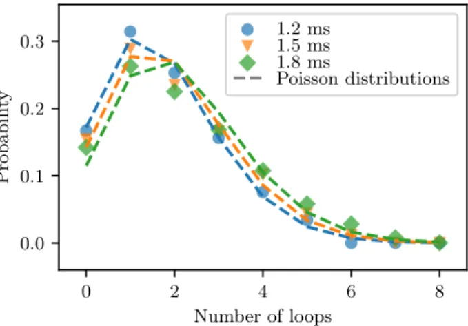
Figure S2. Statistics of the number of loops done by the ran-dom walks described in the text for different ranran-dom walk lengths (symbols) and the corresponding Poisson distribu-tions (dashed lines, the colors encode the path lengths).
II. NUMERICAL SIMULATIONS OF THE NUMBER OF LOOPS IN THE CAVITY
In order to get an estimation of the number of loops done by each closed paths in the cavity, we perform an angular random walk in polar coordinates. The geometry is shown in Fig. S1. The random walks starts at the bottom point (θ = 0), with a random angle, and travels on straight lines between successive scattering events. A scattering event happens each time the random walk crosses the circle. Let us call αi the angle with respect to the normal at which the path impacts the circle, the path then continues with an angleθs which is chosen on a normal law centered on αs=αi(specular reflection) with a certain width (standard deviationσ) accounting for the roughness of the surface. We continue the random walk until the total travel time of the walk is equal to the measured ones (1.2 ms, 1.5 ms or 1.8 ms; radius of the cavity, 7.25 cm; sound velocity, 1500 m/s). We are only interested in the statistics of the backscattered paths, which mean that we only keep the paths which end atθ = 0 after the total travel time. During the random walks, we log the number of loops done by the path around the vortex. Fig. S2 shows an example of the statistics of the number of loops done by 50,000 random walks ending at θ = 0, when σ = 40◦. The dashed lines correspond to the Poisson distributions calculated using the average number of loops extracted from the statistics. The good agreement between the simulated statistics and the corresponding Poisson distributions justifies Eq. (6).
[1] E. Jones, T. Oliphant, P. Peterson, et al., “SciPy: Open source scientific tools for Python,” (2001–), [Online; accessed 02/04/2019].
[2] D. E. Amos, “Algorithm 644: A portable package for Bessel functions of a complex argument and nonnegative order,” ACM Trans. Math. Softw. 12, 265–273 (1986).