Ice-penetrating radar survey of the subsurface debris field at Camp Century, Greenland

Contents lists available atScienceDirect

Cold Regions Science and Technology

Ice-penetrating radar survey of the subsurface debris

field at Camp Century,

Greenland

Nanna B. Karlsson

, William T. Colgan

, Daniel Binder

, Horst Machguth

,

Jakob Abermann

, Karina Hansen

, Allan Ø. Pedersen

a_{Geological Survey of Denmark and Greenland, Copenhagen, Denmark} b_{Asiaq - Greenland Survey, Nuuk, Greenland}

c_{Department of Geosciences, University of Fribourg, Switzerland} d_{Department of Geography, University of Zurich, Zurich, Switzerland}

e_{Climate Research Section, Zentralanstalt for Meteorology and Geodynamics (ZAMG), Vienna, Austria} f_{Department of Geography and Regional Science, University of Graz, Graz, Austria}

A R T I C L E I N F O Keywords: Ice-penetrating radar Debris Camp Century Greenland ice sheet

A B S T R A C T

The warming climate is changing the surface dynamics of the Greenland Ice Sheet, including the balance be-tween snowfall and melt. Increasing surface melt impacts the structure of the relatively porous near-surface layer known asfirn. Camp Century, a base abandoned in 1967, now comprises a subsurface debris field within the firn in Northwest Greenland. We collected 80 km of 100 or 250 MHz radar data in nested grids over this subsurface debrisfield. Here, we present a comprehensive analysis and interpretation of this ice-penetrating radar survey. The vast majority (95%) of subsurface reflectors are located at depths of greater than 32 m. The tunnel network, as well as an overlying layer associated with historical surface activities, is readily visible in the radar data. This subsurface debrisfield is approximately circular with a radius of less than 1 km. Local downwarping of clear internal layers– likely annual accumulation layers - identifies now-collapsed liquid sumps. Analysis of radar signal polarity suggests that liquid hydrocarbons are likely present in one of these sumps. The radar data and a geo-referenced site map of Camp Century are freely accessible atwww.campcenturyclimate.dk.

1. Introduction

Camp Century was constructed in 1959 by the US Army Corps of Engineers as a subsurface base within the Greenland Ice Sheet. It housed up to 200 soldiers and was occupied year-round until 1964. It continued seasonal operations for an additional three summers and was permanently abandoned in 1967. Camp Century was excavated within the relatively soft near-surfacefirn as a cut-and-cover trench network at an initial depth of 8 m (Clark, 1965). Persistent snowfall has now buried the base entirely, leaving nothing visible at the ice-sheet surface. For insights into the political and military history of Camp Century, we refer readers to recent studies (Nielsen et al., 2014;Nielsen and Nielsen, 2016).

Camp Century is located in the northwest corner of the Greenland Ice Sheet, approximately 200 km east of Thule Air Base (Fig. 1). It is situated at 1886 m above sea-level, where ice thickness is 1387 m, with a coastward ice-flow velocity of approximately 4 m/ yr. The mean an-nual air temperature at Camp Century is−24 °C and the mean annual

accumulation rate is 32 cm/ yr ice-equivalent (294 mm w. eq. yr−1) (Steffen and Box, 2001;Buchardt et al., 2012). While Camp Century is presently in the accumulation area, surface mass balance at the site might change to net ablation by 2100 under the UN Intergovernmental Panel on Climate Change (IPCC) RCP8.5“business-as-usual” scenario of greenhouse gas emissions (Colgan et al., 2016;Fettweis et al., 2017). Under the RCP4.5, or approximately “Paris Agreement” scenario, however, net accumulation might persist beyond 2100.

The presence of the Camp Century debrisfield has been confirmed from the airborne radar surveys conducted by NASA. Since 2010, NASA campaigns have included UHF (ultra-high frequency; 565–885 MHz) radar to measure near-surface ice-sheet stratigraphy at sub-meter re-solution (Leuschen et al., 2014;Koenig et al., 2016). While this UHF airborne radar detects unambiguous subsurface reflectors at Camp Century, its along-track sampling of approximately 20 m has been in-sufficient to confidently delineate even large features within the sub-surface debrisfield, including tunnels with a width of 6 m. Even so, the clear internal layering could be utilized to provide estimates of

https://doi.org/10.1016/j.coldregions.2019.102788

Received 12 October 2018; Received in revised form 11 February 2019; Accepted 20 May 2019

⁎_{Corresponding author.}

E-mail address:nbk@geus.dk(N.B. Karlsson).

Available online 20 June 2019

0165-232X/ © 2019 The Authors. Published by Elsevier B.V. This is an open access article under the CC BY license (http://creativecommons.org/licenses/BY/4.0/).

accumulation rates in the area. Additionally, virtually all available airborne profiles are oriented East-West – reflecting transit flights to and from Thule Air Base– which limits 3D analysis of subsurface fea-tures. In comparison to this existing airborne radar data, the new VHF (100–250 MHz) radar data we present here has an approximately 10 cm along-track sampling with decimeter-scale depth resolution (cf.Fig. 2). This increased spatial and vertical resolution provides a transformative improvement in the ability to delineate subsurface debris features.

Due to the concerns of the Government of Greenland over the po-tential remobilization of contaminants at Camp Century, the Government of Denmark established the long-term Camp Century Climate Monitoring Programme in 2017 (Colgan et al., 2017). While this monitoring programme is primarily focused on measuring the depth to which meltwater percolates today, and simulating the depths to which it may percolate in the future, it also includes a one-time survey of the subsurface debrisfield. Here, we use geophysical methods to analyze detailed ice-penetrating radar data collected at Camp Cen-tury, in order to map the horizontal and vertical extents the subsurface debrisfield at the site.

2. Field data

Ice-penetrating radar and ice core data were collected in July and August 2017, when the Geological Survey of Denmark and Greenland deployed a six-person team to Camp Century for two weeks (Colgan et al., 2018). Thule Air Base served as the logistical base for a ski-equipped Twin Otter aircraft supporting the camp. The temporary camp was established within the debrisfield, approximately aligned with the location of post-closure surface camps (Kovacs, 1970). Although de-camped entirely, the approximately 0.25 ha footprint of the 2017 temporary camp will be visible in subsequent ice-penetrating radar surveys most likely due to the formation of massive wind-sculpted snowdrifts around it. All the ice-penetrating radar data described here, as well as other real-time climate and ice measurements, are freely available atwww.campcenturyclimate.dk.

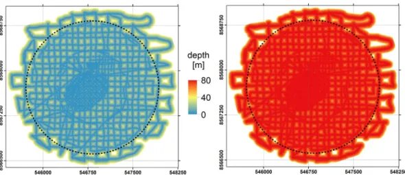
The subsurface debrisfield was surveyed with 80 km of ice-pene-trating radar data (Fig. 1). These data were collected using a Malå shielded antenna (250 MHz) or rough terrain “snake” antenna (100 MHz). The antennas were towed behind a person on cross-country skis who continuously monitored output data in real-time (Fig. 3). A Fig. 1. (A) Location of Camp Century. (B) Ice-penetrating radar survey lines at 250 MHz (blue) and 100 MHz (red) with the location of core B73 (black dot) and core B62 (magenta dot). The map is shown in UTM (Universal Transverse Mercator) zone 20 N using WGS84 (World Geodetic System). (C) As-built map of Camp Century with main structures annotated.

peripheral GPS antenna simultaneously tagged each radar trace with local coordinates to position it within ± 3 m horizontal accuracy. Pri-mary radar acquisition was within two nested grids: a 100 m grid with principle south alignment and a 50 m grid with principle north-west-southeast alignment. The transects comprising these grids were coordinated prior to fieldwork. This was done by geo-referencing a historical site map using a single tie-point corrected for motion since its last precise survey (Kovacs, 1970; Gundestrup et al., 1987). This a priori positional estimate of the subsurface debrisfield turned out to be biased approximately 150 m eastwards (see discussion below). Sec-ondary radar acquisition was performed to verify specific ice-drilling sites as safe and was therefore not conducted in a grid but was targeted around the proposed drill site.

The relatively open porous near-surface ice-sheet layer known as firn has spatially and temporally variable density. As radar velocity is proportional to material density, twofirn density profiles were mea-sured in support of this radar analysis (Colgan et al., 2018). Ice cores were recovered using the University of Wisconsin Eclipse2 ice-drilling system. This relatively lightweight (800 kg) tip-drill system operates without drillingfluid to depths of approximately 300 m (Blake et al.,

1998). A 73 m core (hereafter B73) was drilled inside the debrisfield and a 62 m core (hereafter B62) was drilled 1.5 km southeast, upwind of main wind direction, outside of the debrisfield (Table 1). These cores were analyzed for density, as well as visual stratigraphy to a depth of approximately 65 m, on an open-air processing table (Fig. 4) (Machguth et al., 2016). Core sections were cut into samples of 10.0 cm in length, or 9.9 cm accounting for saw loss, and weighed using a digital scale. Firn density was subsequently calculated using an internal drill dia-meter of 8.0 cm and assumed uncertainties of 0.1 mm in diadia-meter and 0.5 cm in length. The loss or damage of each core section, exclusive of drill chips, was also characterized as an additional fractional un-certainty that was propagated in density calculations. As the ice-drill tips into a drilling trench approximately 2 m deep, the uppermost 2 m of each density profile was sampled as a snowpit. The cores were subse-quently examined off-site for indications of radioactive contamination see (Qiao et al., 2018).

Age-depth relations have previously been estimated for both ice cores by combining measured accumulation-depth profile with decadal accumulation rate history (Qiao et al., 2018). Uncertainties in the ac-cumulation-depth profile and accumulation rate history were assumed to be independent and sum in quadrature to yield total date un-certainty. In core B73, the characteristic age-depth uncertainty in-creases from 2016.8 ± 0.3 CE (Common Era) at 1.80 m depth to 1948.9 ± 1.4 CE at 40.00 m depth and 1873 ± 3.0 CE at 73.00 m depth.

3. Methodology

3.1. Radar processing

During acquisition, multiple ice-penetrating radar traces were au-tomatically stacked to reduce the signal-to-noise ratio. Afterwards, we carried out several processing steps to enhance the visibility of sub-surface reflectors, and thus ensure the best inputs for data interpreta-tion. This processing was carried out with the ReflexW software, and it follows standard procedures in seismic and ground-penetrating radar Fig. 2. A NASA Operation IceBridge (OIB) UHF radar profile (top) intersecting

the Camp Century (CC) area. For comparison the high-resolution ground-based VHF radar is shown below. The dashed black line indicates the intersection between the two radar lines and the black stars show the beginning of the radar lines.

Fig. 3. Acquiring 250 MHz ice-penetrating radar by cross-country ski.

Table 1

Characteristics offirn cores B73 and B62.

B73 B62 Drill date 25/7-17 28/7-17 Latitude (°N) 77.1826 77.1714 Longitude (°W) 61.1125 61.0778 Elevation (mASL) 1886 1885 Depth (m) 73 62

Max. age (CE) 1873 ± 3 1900 ± 3

data analysis (cf.,Navarro and Eisen, 2010;Yilmaz, 2001). First, we removed the DC component of the signal using a window size of 10 ns. Then, we applied a Butterworthfilter with upper and lower cut-offs of 50 MHz and 350 MHz, respectively. In order to enhance the deeper reflectors, we then applied a natural logarithm function. Examples of radar data that have gone through this processing chain are shown in Fig. 5andFig. 6.

The processing steps outlined above, enhance the visibility of re-flectors and accounts for the deterioration of signal strength with depth. However, as visible inFig. 6, other artifacts remain including hyper-bolic signals. This type of artifact is typically caused by a moving an-tenna encountering a very strong reflector at a distance. For example, as an antenna approaches a debris-filled tunnel, the strong oblique returns

will manifest as shallower and shallow nadir returns until the antenna is above the tunnel. Conversely, as the antenna recedes from the tunnel, the increasingly oblique strong returns will manifest as increasingly deep nadir returns.

To account for the classic hyperbole artifact that results from strong oblique returns, we apply a Fk migration using an average velocity of 0.15 m/ns (seeSection 3.3). This processing step– when applied cor-rectly– collapses hyperboles into single point reflectors (Stolt, 1978). Finally, we introduce a small degree of horizontal smoothing by a moving average with a window size of 5 traces. An example of the radar data after these last two processing steps is shown inFig. 7. From this figure, it becomes clear that the apparent hyperbole is caused by a strong point reflector, rather than a spatially extensive reflector. The layering underneath the reflector is unclear, which highlights how shallower reflectors can shadow deeper reflectors.

3.2. Reflector identification

The majority of the identification and mapping of subsurface debris reflectors was carried out in the OpendTect software package. Debris reflectors, including hyperboles and disturbed accumulation layers, were manually identified by comparing their strength to that of sur-roundingfirn. Once identified, the geo-location (x,y,z) of reflectors was recorded for subsequent interpretation. The 3D capabilities of OpendTect allowed for evaluation of cross-over points and identifica-tion of the same reflector in multiple radar lines. In addition to point reflectors associated with debris, three discrete annual accumulation layers at c. 17, 38 and 63 m depth– tentatively assigned dates of c. 1993, 1964 and 1889– were also traced across the survey area (Clausen et al., 1988). These continuous reflecting layers were used to highlight downwarping associated with the collapse of waste sumps.

3.3. Depth conversion

Radar data are inherently recorded as two-way travel time that must be subsequently converted to depth. This depth conversion is aided by the density measurements from the twofirn cores drilled in the survey area. We assume that the speed of the radar waves may be approxi-mated by (Eisen et al., 2006):

Fig. 5. Example of a radargram from the 250 MHz antenna from an undisturbed part of the survey area. The horizontal lines are most likely annual snow ac-cumulation layers. The radargram is expressed in depth (left) and two-way travel (TWT) time (right). The map inset indicates the location of the radargram (thick black line).

Fig. 6. Example of a radargram from the 250 MHz antenna with a clear strong reflector (black arrow) and indications of a surface that has been modified by activity (white arrow). The less distinct horizontal lines are most likely annual snow accumulation layers. The radargram is expressed in depth (left) and two-way travel (TWT) time (right). The concave up parabolas are noise probably caused by a ringing in the antenna system. The map inset indicates the location of the radargram (thick black line).

Fig. 7. The radargram shown inFig. 6after Fk migration. A clear strong re-flector (black arrow) and indications of a surface that has been modified by activity (white arrow). The less distinct horizontal lines are most likely annual snow accumulation layers. The radargram is expressed in depth (left) and two-way travel (TWT) time (right). The map inset indicates the location of the ra-dargram (thick black line).

= ′ v z c ε z ( ) ( ) 0 (1) where c0is the speed of light in vacuum andε′the relative permittivity.

In order to obtain a reliable permittivity, and thereby determine the location of reflections at depth, we apply the real-valued Looyenga mixing model (Looyenga, 1965)

⎜ ⎟ ′ = ⎛ ⎝ ′ − + ⎞ ⎠ ε z ρ z ρ ε ( ) ( )[ 1] 1 i i 3 3 (2) The density with depth,ρ(z), is constructed as a smoothed average from the in-situ measurements. The values for density and permittivity of pure ice areρi= 917 kg m−3andεi′= 3.15, respectively. The latter

value is derived from bothfield measurements and laboratory studies (Eisen et al., 2006; Bohleber et al., 2012). The resulting velocity is shown inFig. 8.

3.4. Reflector characterization

In addition to the depth of a reflector, it is also possible to deduce whether liquid water or hydrocarbon is present based on characteristics of the returned signal. For example, the presence of subglacial lakes is inferred from ice-penetrating radar as an exceptionallyflat and smooth reflection (Oswald and de Robin, 1973; Siegert, 2005). Additionally, the large contrast in electromagnetic impedance between water and glacial ice causes a strong reflection of the radar waves (Carter et al., 2007). Following (Lane et al., 2000) we consider the reflection coeffi-cient R that describes the amplitude and polarity of the radar wave reflected from an interface between two materials

= − + R μ ε μ ε μ ε μ ε 2 2 1 1 2 2 1 1 (3)

where ε is the dielectric constant (relative permittivity) and μ the magnetic permeability of the two materials. If R is negative, the re-flection will have an opposite phase as the emitted wave. If R = ± 1, the signal is reflected fully, while a value of zero indicates total ab-sorption of the wave. The magnetic permeability of snow, ice and hy-drocarbons is very similar to that of air (Lane et al., 2000). The

dielectric constant of snow or ice and hydrocarbons is close in value (between 1 and 3), while the value for liquid water is substantially higher (cf.Table 2). Thus, an interface betweenfirn and liquid water will reverse the polarity. An interface betweenfirn and glycol could, depending on type of glycol and the density of the firn, reverse the polarity. However, the reflection would be significantly weaker than that resulting from a water-firn interface (cf. Eq.(3)). This allows us to get an indication of whether a reflection is due to liquid water or hy-drocarbons.

4. Data interpretation

4.1. Historical active surface

Surface activities during the years that Camp Century was active have disturbed the surface in a fashion that is readily identifiable in both the radar andfirn core data. The firn core data indicate that near-surfacefirn densities are similar both inside and outside the debris field to 32 m depth. Between 32 and 35 m depth,firn density is substantially greater inside the debrisfield. In this depth range, densities inside the debrisfield approach that of pure ice (888 kg m−3_{at 33.35 m depth)}

while those outside the debrisfield are < 700 kg m−3. This high-den-sity layer, which is discolored slightly yellow in appearance and con-tains visible macroscopic particulates, likely reflects enhanced local compaction and pollution during the Camp Century active period. Below this active layer,firn densities are similar inside and outside the debrisfield. We employ the age-depth relation described inSection 2 and its associated uncertainty and from thisfirst-order age-depth rela-tion we get that the active layer corresponds to the c. 1959 to 1965 period (Qiao et al., 2018). While the ice-sheet wide 2012 melt layer is evident at Camp Century (Nghiem et al., 2019), thefirn stratigraphy is now comprised of widely-spaced thin ice layers characteristic (see Fig. 11) of a shallow percolationfirn regime (Machguth et al., 2016). As an additional check of the age-depth relationship, we count the number of layers from the active layer to the surface and get an estimated 72 layers. If all layers were annual layers, we would expect between 52 and 58 layers. Likely, the reflections in the upper 5–10 m are caused by sub-annual density variations accounting for the high number of layers. The radar data suggests that this historical surface activity layer sampled by core B73 is widespread across the debrisfield. The sub-surface debrisfield characterized by this layer is approximately circular with a radius of less than 1 km. The largest number of radar reflectors are identified in the depth range 35 m to 45 m. (Fig. 9). This depth range corresponds to the historical surface activities and the underlying tunnel network. Past modification of the snow comprising the historical active surface has evidently created a sharp dielectric contrast with both under- and over-lying undisturbed snow. An example of this re-flector characteristic can be seen inFig. 6 andFig. 7 marked with a white arrow. Another near-surface feature that consistently appears is an area with several reflecting horizons (Fig. 10; turquoise arrow). This thick-disturbance layer is typically encompassed by upper and lower horizontal reflectors with multiple strong reflectors between. We hy-pothesize that this is either a remnant of the former surface camp used to construct Camp Century, or an area to where excess snow was cleared during camp operations, or a combination of both. The thick-Fig. 8. (A) Measured densities fromfirn core B73 showing disturbed firn inside

the debris field (blue), and firn core B62 outside the debris field with un-disturbedfirn (orange). (B) The corresponding calculated radar wave speed and the average speed (black). (For interpretation of the references to colour in this figure legend, the reader is referred to the web version of this article.)

Table 2

Dielectric permittivity.

Material Dielectric constantε′ _Reference

Snowa _{1− 4 (Navarro and Eisen, 2010;Kovacs et al., 1995)}

Ice 3− 4 (Plewes and Hubbard, 2001)

Water 80 (Plewes and Hubbard, 2001) Glycolb _{2.9− 6.3 (Sengwa et al., 2019)}

a

Values depend on snow density.

disturbance area extends 1.5 km east-west and 0.5 km in north-south, with an approximate depth between 35 m and 45 m. In many radar lines we can also identify strong reflectors in this depth range that appear to be single point reflectors. These point reflectors can be caused by a number of processes, but one likely explanation is small-scale debris left on the historical surface, such as old cables or empty fuel drums (Fig. 10; red arrow).

4.2. Infrastructure reflectors

The main camp infrastructure– tunnels – are identified in the 45 m to 55 m depth range, immediately beneath the layer associated with historical surface activities (Fig. 9). The central part of the survey area is concentrated on the primary tunnel network. Abandoned infra-structure is clearly visible in the ice-penetrating radar data from this part of the survey area. The radar is most likely detecting any remaining

metal ceiling forms used in cut-and-cover trench construction, as well as the utility conduits lining tunnels. These spatially dense reflectors permit a relatively accurate delineation of the present-day tunnel lo-cations (Fig. 12). The space-depth relation of reflectors associated with Fig. 9. Histogram of the depth distribution of all identified radar reflectors.

Labels denote populations of reflectors discussed in the text.

Fig. 10. Left: Example of radargram where historical surface activity is clearly visible. The turquoise arrows indicate the upper and lower boundaries of the historical active surface layer. The red arrow indicates a single strong reflector identified within the disturbed firn. Right: Maps of the extent of the thick-dis-turbance layer and the single reflectors, respectively. (For interpretation of the references to colour in this figure legend, the reader is referred to the web version of this article.)

Fig. 11. Left: Density of the B73 smoothed with a running average. Center: Observed ice lenses (blue) and active layer (yellow). Right: The age-depth re-lation as calculated by (Qiao et al., 2018). (For interpretation of the references to colour in thisfigure legend, the reader is referred to the web version of this article.)

Fig. 12. Example of a radargram intersecting the main tunnel network (upper: processed, lower: processed and migrated). Upper radargrams: The blue arrows indicate the location of buried camp structures, the turquoise arrow the upper boundary of the thick-disturbance layer, the white arrow the historical active surface, and the black arrow an unidentified shallow reflector. Lower radar-gram: Colored arrows indicate the buried camp structures corresponding to the colored lines in the right-hand panel. Right: Maps of the extent of reflectors of the main tunnel network. The magenta line depicts the radargram line. (For interpretation of the references to colour in thisfigure legend, the reader is referred to the web version of this article.)

camp structures is shown inFig. 13. The main tunnels are now located at a depth of approximately 48–50 m, which is deeper than previously estimated (Colgan et al., 2016). This is consistent with an initial cut-and-cover depth of 8 m below the historical surface activities layer (Clark, 1965). The radar reflectors become shallower – averaging just 46 m depth– in the northeast corner of the tunnel network. This is consistent with the location of tunnels housing the nuclear reactor, which had significantly higher ceiling heights than other tunnels. The horizontal extent of the mapped tunnel network is approximately 500 m by 500 m, including the secondary tunnels east of the primary tunnel network. There is no radar evidence for the presence of tunnels not depicted on the as-built site map (Kovacs, 1970). There is also no radar evidence for unmapped sanitary landfills and runway infrastructure within the survey grid.

Additional infrastructure reflectors are identified both above and below the 45 m to 55 m depth range of the main tunnel network. Below the main tunnel network, there are a small number of deeper reflectors that are up to 130 m deep (Fig. 14). The majority of these deeper re-flectors, however, are between 55 m and 70 m (Fig. 15). We hypothe-size that the very deepest reflectors (130 m deep) are associated with the glycol sump. The characterization of these deepest glycol sump reflectors is discussed below inSection 4.3. It is important to note that the majority of radar data was collected with the 250 MHz antenna, which only images reflectors down to approximately 80 m. It is the only relatively few radar lines collected with the lower frequency and deeper penetrating 100 MHz antenna that can potentially resolve reflectors below this depth. The 100 MHz data collection was limited tofinding a suitable site for ice-drilling through the debris field. As the tunnel network resides at depths of less than 55 m, the higher resolution but shallower penetration of the 250 MHz antenna was generally preferred to the lower resolution and deeper penetration of the 100 MHz antenna. While the vast majority (95%) of all identified infrastructure reflectors are located at depths greater than 32 m, there are a small number above the historical active surface. These shallower near-surface reflectors generally appear at depths of between 20 m and 25 m, but a few re-flectors are identified at even shallower depths. All shallow near-sur-face reflectors appear to be single point reflectors. An example of such a reflector is marked with a black arrow inFig. 12. The nature of these shallow near-surface reflectors is unknown, but they could be objects

down to the size of a cable or fuel drum. A preliminary age estimate of the 20 m to 25 m depth range suggests it dates between 1979 and 1987. These reflectors are likely either associated with post-closure research activities at the site (Gundestrup et al., 1987; Thomas et al., 2001; Hawley et al., 2014), or massive snowdrifts that persisted after aban-donment, or both. The majority of post-1990 Program for Arctic Re-gional Climate Assessment (PARCA) activities within the vicinity of Camp Century actually occurred approximately 5 km SE at GITS and are therefore unlikely to have further disturbed the debrisfield (Steffen and Box, 2001; Mosley-Thompson et al., 2001; Hamilton and Whillans, 2002).

Fig. 13. Depth of radar reflectors identified as associated with the tunnel network overlaid on a geo-referenced as-built map of Camp Century (Fig. 23). Radar survey lines are shown in gray. The map is in UTM zone 20.

Fig. 14. Example of a radargram intersecting the main tunnel network where a deep reflector (red arrow) is visible. The turquoise arrow indicates the upper boundary of the thick-disturbance layer, and the blue arrow one of the tunnels. Right: Map of the extent of the deep reflectors below the main tunnel network (top) and map showing the location of the radargram. (For interpretation of the references to colour in thisfigure legend, the reader is referred to the web version of this article.)

4.3. Liquid phase reflectors

In the following, we analyze the deepest reflectors visible in the 100 MHz data in order to elucidate the nature of the reflector. We do this by a quantitative analysis of the signal polarity. Firstly, we note that the reflectors are likely either ice, metal, air, water or glycol. We do not consider ice a very probable candidate since the dielectric contrast between firn and ice should not be big enough to cause a strong re-flection. If the reflection is caused by a metal roof over a cavity then we would not expect to observe a large subsidence. In contrast, if the cavity is air-filled with no metal roof, we would expect a subsidence. If the dimensions of such an air cavity do not exceed a few wavelengths (for a frequency of 100 MHz the wavelength is∼2 m), we would observe a strong reflection due to the superposition of the top and the bottom reflection signal. We cannot rule out that the reflector is an air cavity, however, we would also expect such a cavity to havefilled in by now. We therefore consider it likely that the strong reflectors are either water, glycol or a mix of the two. Theoretically, the presence of liquid water induces a change in radar waveform polarity, while the presence of liquid hydrocarbon induces a strong reflection but no change in polarity. Before we explore the signal properties further, we note that a change in polarity may also be caused by propagation through a medium depending on the properties of the medium such as its roughness and scattering properties. Ideally, detailed information on thefirn density is required to fully compute the resulting signal e.g., [21]. While we do not have such information, it is well known that snow/firn stratigraphy is laterally very smooth and homogeneous. In our study area, thefirn stratigraphy appear flat and smooth over 10s to 100 s of meters. We therefore consider it unlikely that the signal has been modulated due to surface roughness. Similarly, scatterers have a dominant effect on the signal if the dimension of the single scatterer, or a cluster of scatterers, is of the same scale as the apparent wavelength. Thus to influence our observations, scatterers must be of the scale of a few meters. Apart from the camp infrastructure, we do not expect the firn to contain single scatterers of this spatial scale. In summary, while we cannot rule out that the propagation through thefirn may cause a change in signal polarity, given the arguments above we consider it likely that the signal polarity of our data is retained.

Fig. 16shows the A-scope at four different depths of a single trace.

The surface reflection (from the air/snow interface) is used as a baseline for the polarity of the emitted radar signal. Here, we see thefirst and strongest reflection has a positive value. The signal intercepts several strong reflectors (turquoise and yellow) before encountering the very deep reflector (blue). Both the intermediate and deep reflectors do not reverse the polarity of the signal. We interpret this as an indication of the presence of hydrocarbons rather than water. We therefore consider it likely that this sump is the glycol depot. This is consistent with the observation that pressurized hydrocarbon vapors vented from borehole B73 (approximately 50 m away) (Colgan et al., 2018). The mean annual air temperature at Camp Century, and therefore the approximate ice temperature below 12 m depth, is −24 °C. As the freezing point of glycol is substantially lower (−59 °C for propylene glycol), there is a theoretical expectation that the glycol sump indeed remains liquid.

We observe one location where there is an indication of signal Fig. 15. Depth of deepest identified radar reflectors associated with infrastructure overlaid on a geo-referenced as-built map of Camp Century (Fig. 23). Radar survey lines are shown.

Fig. 16. Example of a 100 MHz radargram and four A-scopes at different depths indicating potential liquid hydrocarbon at 130 m depth in the vicinity of the glycol sump.

polarity reversal. An example is shown inFig. 17, where the reflector at approximately 46 m depth (turquoise colors) could be interpreted as a signal reversal. In addition, the signal below this reflection are sub-stantially weaker. This may indicate liquid water pooled above the impermeable historical active surface. We cannot, however, dissect whether the water is mixed with glycol. The potential liquid water trace of Fig. 17 is also located within the glycol sump downwarping, ap-proximately 50 m from the potential liquid hydrocarbon trace of Fig. 16. Analogous radar indications of liquid water pooled in a downwarped depression of the historical active surface are also iden-tified in intersecting 250 MHz radar data (Fig. 18, yellow colors).

Summer meltwater percolation at Camp Century presently appears

to be restricted to within the annual accumulation layer (within ap-proximately 1 m of the ice-sheet surface) (Colgan et al., 2018). Else-where on the ice sheet– in more melt prone regions of the accumulation areas– summer meltwater percolation has been observed to reach a maximum of 10 m depth (Humphrey et al., 2012). It is therefore highly unlikely that these indications of liquid water at 46 m depth in other-wise−24 °C ice are associated with deep meltwater percolation. Ob-servations– including in ice-sheet sewage sumps – and theory suggest that the tremendous latent heat energy released by refreezing water means it can take several years to decades for massive liquid water volumes in otherwise cold ice to refreeze (Bader and Small, 1955; Ostrom et al., 1962;Jarvis and Clarke, 1974;Clarke and Jarvis, 1976; Phillips et al., 2010). We therefore consider it likely that any liquid water at depth is relict water associated with camp activities.

5. Discussion

5.1. Radar resolution

While radar observes the complete surface-to-extinction depth profile along-track, the observed depth range in adjacent across-track ice is dependent on track-perpendicular distance. The 250 MHz antenna was operated with a time window of 682 ns corresponding to ap-proximately 80 m (depending on snow density). Assuming a radar il-lumination angle of 120° and a radar energy extinction length of 80 m, we can calculate the uppermost and lowermost ice depths observed by the 250 MHz antenna across the debrisfield (Fig. 19). This sensitivity analysis suggests that we have observed the uppermost active layer (c. 1967 or 31 m) across 95% of a 3.80 km2_{circular search area of radius}

1.1 km. Within this search area, the lowermost observable ice depth generally approaches our assumed radar energy extinction depth of 80 m. There are regions between widely spaced tracks, however, where the convergence of adjacent uppermost observable depths creates plunging radar shadows that approach 30 m depth (Fig. 20). Vertically-stacked debris, whereby shallower debris attenuates radar energy be-fore reaching deeper debris, creates irregular radar shadows within these idealized bounds. Generally, we believe that all large-scale debris – that with a length dimension greater than 10 m – has been observed within the circular search area. Unobserved debris of smaller length dimension may be present above or below the uppermost or lowermost observable ice depths, respectively, or in radar shadows within this area.

5.2. Downwarping

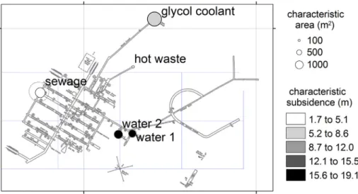
At Camp Century, liquids were stored in unlined sumps that reached substantially greater depths than the solid tunnel infrastructure. The subsequent deformational closure of these sumps has resulted in sub-stantial, but spatially variable, downwarping of annual accumulation layers within the debris field. This downwarping is the result of the initially air-filled head space of these sumps deforming closed through syncline collapse of overlyingfirn layers (Fig. 21). The deformational closure of tunnels has also contributed to spatially variable down-warping, but to a lesser degree and at much shallower depths. We es-timate the characteristic geometry and subsequent subsidence offive known unlined sumps at Camp Century (Table 3,Fig. 22). This estimate is not based on our radar observations but on historical estimates of sump depth, ice removed or waste deposited, and sump geometry– where available – and assuming spherical geometry (Clark, 1965; Colgan et al., 2016;Bader and Small, 1955;Rodriguez, 1963). For the two water sumps, we base our estimates of sump volume on the 13,300 and 19,000 m3 of air headspace associated with drinking water removal reported in (Clark, 1965). For the sewage sump, we base our estimate of sump volume on the 2.4 × 107_{L waste volume reported in (Colgan}

et al., 2016) augmented by the ice melt anticipated from sensible heat release assuming a temperature of 25°. For the hot waste sump, we base Fig. 17. Example of a 100 MHz radargram and four A-scopes at different depths

indicating potential liquid water at 46 m depth in the vicinity of the glycol sump.

Fig. 18. Example of a 250 MHz radargram and two A-scopes, where the deepest one indicates potential liquid water at 46 m depth in the vicinity of the glycol sump. This 250 MHz profile intersects with the 100 MHz profile shown in Fig. 17.

our estimate of sump volume on the waste discharge of 1.8 × 105_{L per}

year discharge rate reported in (Clark, 1965) applied over four years and augmented by the ice melt anticipated from sensible heat release assuming a temperature of 75°. For the glycol coolant sump, we base our estimate of sump volume on the 7.6 × 107_{L liquid volume reported}

in (Clark, 1965). Based on the approximately 25% headspace air vo-lume of the glycol coolant sump reported by (Clark, 1965), we assume equivalent fractional headspace air volumes in the sewage and hot waste sumps. Based on the assumption of three months residual drinking water supply in water sumps 1 and 2 (Colgan et al., 2016), we estimate 84 and 88% headspace air volumes in these respective sumps. While the sump volume estimates we present account for the sen-sible heat release, they neglect the sump growth expected from melt of the surrounding ice by latent heat released from refreezing waste. These order estimates of sump volume are simply meant to facilitate first-order estimates of local subsidence over each sump, and thus aid in the interpretation of radar reflections associated with deep sumps. The two water sumps have the largest characteristic subsidence due to their persistent ice removal. Given their present-day depths – in excess of 150 m– the available radar data cannot fully resolve their deepest ex-tent. In contrast, downwarping associated with the shallower sewage and glycol sumps are clearly apparent in the radar data (Fig. 16), with the sewage sump exhibiting substantially less downwarping (in agree-ment with estimates, cf. Table 3). The relatively small volume, and therefore subdued associated downwarping, of the hot waste sump prohibits confidently identifying its depth or location with the radar data. The deepest reflectors observed in the radar data are positionally consistent with unlined sumps, and therefore unlikely to represent

unmapped solid infrastructure. Based on overlying layers, it appears that the collapse of the water sumps continued for another∼30 years after Camp Century was abandoned. Thus, the headspace is thought to have stabilized by c. 1990. In contrast, downwarping over the glycol sump is either ongoing or has ceased recently, as even near-surface layers appear to exhibit a small degree of downwarping. The analogous collapse and downwarping of smaller tunnel void spaces was likely complete by c. 1980 (Kovacs, 1970).

5.3. Site displacement

We use reflectors associated with infrastructure in the tunnel net-work, as well as reflectors associated with the water, sewage, and glycol sumps to geo-reference an as-built map of Camp Century. The as-built map of Camp Century we employ differs from more numerous and widely available as-planned maps. While the latter are typically limited to the closely-spaced primary tunnel network built in 1959–1960, the former also includes additional secondary tunnels subsequently ex-cavated to the east of the main tunnel network (Clark, 1965;Kovacs, 1970). We use a 2D transformation in the ArcMap software to minimize misfit between the three sump locations on the as-built map and the best radar-derived estimates of their current locations (Fig. 22). Misfit between tunnel infrastructure reflectors and the as-built map is then minimized by manually shifting the as-built map (Fig. 13). The re-sulting geo-referenced map is positionally consistent with infrastructure and sump radar reflections, as well as the absolute distance scale of the original map (Kovacs, 1970). We estimate that this geo-referenced site map– characteristic of the Camp Century debris field in August 2017 – Fig. 19. The uppermost (left) and lowermost (right) observable depths assuming a 250 MHz radar illumination angle of 120° and a radar extinction length of 80 m. The dashed line indicates a 3.8 km2_{circular search area of radius 1.1 km.}

Fig. 20. Idealized 250 MHz radar penetration assuming a radar illumination angle of 120°, a radar extinction length of 80 m and a grid spacing of 100 m.

has a horizontal positional accuracy of ± 20 m (Fig. 23). This positional uncertainty reflects the aggregate of uncertainty in the original site map rendering, uncertainty in contemporary tie-point locations, and un-certainty in intervening differential ice flow and shear across the site. This geo-referenced map places the subsurface debris field approxi-mately 150 m further westward than has been estimated in recent studies (Colgan et al., 2016;Colgan et al., 2017;Colgan et al., 2018). The combination of the radar reflectors and the geo-referenced map also indicate the present position of the radio-meteorological tower. Based on historical satellite-surveyed positions of the tower and its geo-referenced 2017 position ( ± 20 m), we estimate a long-term velocity of 4.0 ± 0.7 m/yr and azimuth of 256 ± 2° during 1986–2017 and 3.9 ± 0.5 m/yr at 253 ± 2° during 1977–2017 (Gundestrup et al., 1987). These displacement vectors deviate slightly from the 3.8 m/yr at 234° satellite-surveyed at CEN-GPS in 1995–1996 (Thomas et al., 2001) (Fig. 23). We estimate that iceflow has displaced Camp Century ap-proximately 232 m WSW– with a 4° clockwise rotation – between site construction in 1959 and our resurvey in 2017. The August 2017 geo-referenced site map of Camp Century is available on the project website www.campcenturyclimate.dk. To fully assess the horizontal and ver-tical movement of the debrisfield, detailed information is needed on present and future ice-flow velocities and surface mass balance. This information is currently uncertain (e.g., direction of current ice-flow velocity) or unknown (e.g., future surface mass balance). Our measured displacement rates indicate that the debris field is currently moving

approximately 400 m per century. Towards the margin, the ice-flow speeds increase but due to the camp position on the ice divide, the debris field is far from those fast flow areas. Indeed, velocities only exceed 20 m/yr more than 20 km from the debrisfield. At the margin of the ice-sheet, there are several small outlet glaciers but areas with ve-locities above 500 m/yr only extend a few tens of kilometers inland. Further assessment of the long-term ice dynamics is outside the scoce of this radar survey.

6. Summary remarks

The Camp Century Climate Monitoring Programme has completed a one-time ice-penetrating radar survey of the subsurface debrisfield at Camp Century. The survey comprised of 80 km of 100 or 250 MHz radar data collected in nested grids over this subsurface debrisfield during July and August 2017. Our sensitivity analysis suggests an uppermost observable depth of 31 m (or c. 1967) across 95% of a 3.8 km2_circular

search area of radius 1.1 km. The lowermost depth generally ap-proaches 80 m, although vertically-stacked debris contributes to sub-stantial radar shadowing. While some radar reflectors are present within 20 m of the ice-sheet surface, the vast majority (95%) of sub-surface reflectors are located at depths of greater than 32 m. In the context of projecting future meltwater percolation, it is important to note that this critical depth is specific to 2017, and will increase with the net snow accumulation of coming years to decades.

Fig. 21. Idealized isochrone downwarping due to sump col-lapse between 1964 and 2017. The idealized sump geometry approximates that of the sewage sump and is scaled to the tunnel. The thick isochrone highlights the historical active surface in both plots. Subsidence denoted with an arrow. *For liquid wastes with freezing points above−24 °C that even-tually reach thermodynamic equilibrium with surrounding ice temperatures over years or decades.

Table 3

Characteristic geometry and subsidence estimates forfive unlined sumps at Camp Century based on historical literature and the assumption of spherical geometry. Sump volume– the total of both liquid waste and air headspace volumes – accounts for the sensible, but not the latent, heat release associated with sump contents.

Water 1 Water 2 Sewage Hot waste Glycol Top depth 1964 (m) 152 ± 10 166 ± 10 33 ± 10 56 ± 20 56 ± 5 Top depth 2017 (m) 180 ± 15 194 ± 15 61 ± 15 84 ± 25 84 ± 10 Liquid volume (103_m3_{) 2.6 ± 1.3 2.6 ± 1.3 32 ± 6.3 1.4 ± 0.28 76 ± 15} Air volume (103_m3_{) 13 ± 2.7 19 ± 3.8 7.9 ± 1.6 0.35 ± 0.07 19 ± 3.8} Sump volume (103_m3_{) 17 ± 4.3 24 ± 5.6 43 ± 8.6 1.9 ± 0.38 100 ± 21} Spherical radius (m) 16 ± 1.2 18 ± 1.3 22 ± 1.4 7.7 ± 0.48 29 ± 1.8 Circular area (m2_{) 810 ± 130 990 ± 150 1500 ± 190 180 ± 20 2700 ± 350} Subsidence (m) 16 ± 20 19 ± 25 5.3 ± 8.2 1.9 ± 2.9 7.1 ± 11

The historical active surface– characterized as highly compacted and slightly discoloredfirn – is readily visible in both radar and firn core data at a depth of approximately 32 to 35 m. Below this, radar reflections associated with tunnel network infrastructure are evident at depths of 45 to 55 m. All the tunnels depicted in the as-built map of Camp Century can be identified in radar reflections; there is no evi-dence for unmapped tunnels. The horizontal extent of the mapped tunnel network is approximately 500 m by 500 m, including both the primary and secondary tunnel network. The entire subsurface debris field – including the historical active surface and the thick-disturbance layer – is approximately circular with a radius of less than 1 km. We estimate that 3.9 ± 0.6 m/yr at 255 ± 2° iceflow has now displaced Camp Century approximately 232 m WSW– with a 4° clockwise rota-tion– since its construction in 1959.

The downwarping of clear internal layers within the firn – likely annual accumulation layers– identify now-collapsed liquid sumps that once stored water, sewage, glycol and hot waste. The uppermost depth of the sumps is likely deeper than 80 m, making it virtually impossible to probe these sumps with the 250 MHz radar capable of imaging the shallower tunnel network. Analysis of single-trace 100 MHz radar

polarity in the vicinity of the glycol sump suggests liquid hydrocarbons are likely present at 130 m depth and liquid water is likely present at 46 m depth. These indications of relic liquid wastes, as well as the re-lease of pressurized hydrocarbon vapors from borehole B73, highlight a need for caution when drilling within the debrisfield. We provide a geo-referenced site map of Camp Century, with an estimated horizontal positional accuracy of ± 20 m, in the Supplementary material of this publication.

Camp Century has taken on renewed and unanticipated social sig-nificance in light of climate change. The one-time ice-penetrating radar survey of the subsurface debrisfield presented here facilitates a science-based discussion of the shifting fate of Camp Century. The Camp Century Climate Monitoring Programme is specifically tasked with regularly updating annual likelihoods of meltwater interacting with the debrisfield over the next century. Knowledge of the spatial and depth distribution of the present-day debrisfield, as well as the nature of li-quid wastes, provides a valuable baseline for simulations of future changes infirn structure. At the broadest level, a better understanding of the implications of climate change on Camp Century will perhaps provide a better understanding of the importance of mitigating Fig. 22. The location and characteristic area and subsidence offive known unlined sumps overlaid on an as-built map of Camp Century (Kovacs, 1970).

Fig. 23. As-built map of Camp Century geo-referenced to August 2017 position using radar data (Kovacs, 1970). Esti-mated horizontal positional accuracy is ± 20 m. Camp Cen-tury Climate Monitoring Programme instrument locations denoted in green (Colgan et al., 2018). Velocity estimate de-rived from historical positional surveys denoted in blue (Gundestrup et al., 1987). (For interpretation of the references to colour in thisfigure legend, the reader is referred to the web version of this article.)

greenhouse-gas emissions, and averting, rather than adapting to the consequences of business-as-usual climate change.

Acknowledgements

The radar data and the georeferenced map presented in this pub-lication, as well as near-real-time climate and ice measurements, are freely accessible atwww.campcenturyclimate.dk. 1The radar data may also be found and cited with the DOI: 10.22008/promice/data/icepe-netratingradar/campcentury. The August 2017 geo-referenced site map of Camp Century is available in the Supplementary material of this publication. The Camp Century Climate Monitoring Programme is jointly funded by the Geological Survey of Denmark and Greenland (GEUS) and the Danish Cooperation for Environment in the Arctic (DANCEA) within the Danish Ministry for Energy, Utilities and Climate. J.A was supported by the Greenlandic Ministry of Independence, Foreign Affairs and Agriculture. We warmly thank Mike Jayred for ice-drilling assistance in thefield.

References

Bader, H., Small, F., 1955. Sewage disposal at ice cap installations. In: Snow, Ice and Permafrost Research Establishment Report. vol. 21. pp. 4.

Blake, E., Wake, C., Gerasimoff, M., 1998. The eclipse drill: a field-portable intermediate-depth ice-coring drill. J. Glaciol. 44, 175–178.

Bohleber, P., Wagner, N., Eisen, O., 2012. Permittivity of ice at radio frequencies: part ii. artificial and natural polycrystalline ice. Cold Reg. Sci. Technol. 83–84, 13–19.

https://doi.org/10.1016/j.coldregions.2012.05.010. http://www.sciencedirect. com/science/article/pii/S0165232X12001103.

Buchardt, S., Clausen, H., Vinther, B., Dahl-Jensen, D., 2012. Investigating the past and recent delta 18O-accumulation relationship seen in Greenland ice cores. Clim. Past 8, 2053–2059.

Carter, S.P., Blankenship, D.D., Peters, M.E., Young, D.A., Holt, J.W., Morse, D.L., 2007. Radar-based subglacial lake classification in Antarctica. Geochem. Geophys. Geosyst. 8.https://doi.org/10.1029/2006GC001408.

Clark, E., 1965. Camp Century evolution of concept and history of design construction and performance. Cold Regions Res. Eng. Lab. Tech. Rep. 174, 66.

Clarke, G., Jarvis, G., 1976. Post-surge temperatures in Steele glacier, Yukon territory, Canada. J. Glaciol. 16, 261–267.

Clausen, H., Gundestrup, N., Johnsen, S., Bindschadler, R., Zwally, J., 1988. Glaciological investigations in the Crete area, Central Greenland: a search for a new deep-drilling site. Ann. Glaciol. 10, 10–15.

Colgan, W., Machguth, H., MacFerrin, M., Colgan, J.D., van As, D., MacGregor, J.A., 2016. The abandoned ice sheet base at Camp Century, Greenland, in a warming climate. Geophys. Res. Lett. 43 (15), 8091–8096. arXiv. https://doi.org/10.1002/ 2016GL069688. https://agupubs.onlinelibrary.wiley.com/doi/abs/10.1002/ 2016GL069688.

Colgan, W., Andersen, S., van As, D., Box, J., Gregersen, S., 2017. New programme for climate monitoring at Camp Century, Greenland. Geol. Surv. Denmark Greenland Bull. 38, 57–60.

Colgan, W., Pedersen, A., Binder, D., Machguth, H., Abermann, J., Jayred, M., 2018. Initialfield activities of the Camp Century climate monitoring programme in Greenland. Geol. Surv. Denmark Greenland Bull. 41, 75–78.

Eisen, O., Wilhelms, F., Steinhage, D., Schwander, J., 2006. Instruments and methods: improved method to determine radio-echo sounding reflector depths from ice-core profiles of permittivity and conductivity. J. Glaciol. 52, 299–310.

Fettweis, X., Box, J., Agosta, C., Amory, C., Kittel, C., Land, C., van As, D., Machguth, H., Galleé, H., 2017. Reconstructions of the 1900–2015 Greenland ice sheet surface mass balance using the regional climate mar model. The Cryosphere 11, 1015–1033. Gundestrup, N., Clausen, H., Hansen, B., Rand, J., 1987. Camp Century survey 1986. Cold

Reg. Sci. Technol. 14 (3), 281–288. https://doi.org/10.1016/0165-232X(87)90020-6. http://www.sciencedirect.com/science/article/pii/0165232X87900206.

Hamilton, G., Whillans, I., 2002. Local rates of ice-sheet thickness changes in Greenland.

Ann. Glaciol. 35, 79–83.

Hawley, R., Courville, Z., Kehrl, L., Lutz, E., Osterberg, E., Overly, T., Wong, G., 2014. Recent accumulation variability in Northwest Greenland from ground-penetrating radar and shallow cores along the Greenland inland traverse. J. Glaciol. 60, 375–382.

Humphrey, N., Harper, J., Pfeffer, T., 2012. Thermal tracking of meltwater retention in Greenland's accumulation area. J. Geophys. Res. 117 (F01010).

Jarvis, G., Clarke, G., 1974. Thermal effects of crevassing on Steele glacier, Yukon ter-ritory, Canada. J. Glaciol. 13, 243–254.

Koenig, L., Ivanoff, A., Alexander, P., MacGregor, J., Fettweis, X., Panzer, B., Paden, J., Forster, R., Das, I., McConnell, J., Tedesco, M., Leuschen, C., Gogineni, P., 2016. Annual Greenland accumulation rates (2009–2012) from airborn snow radar. The Cryosphere 10, 1739–1752.

Kovacs, A., 1970. Camp century revisited: a pictorial view - Jun 1969. Cold Reg. Res. Eng. Lab. Special Rep. 150, 42.

Kovacs, A., Gow, A.J., Morey, R.M., 1995. The in-situ dielectric constant of polarfirn revisited. Cold Reg. Sci. Technol. 23, 245–256.

Lane, J.W., Buursink, M.K., Haeni, F.P., Versteeg, R.J., 2000. Evaluation of ground-pe-netrating radar to detect free-phase hydrocabons in fractured rocks– results of nu-merical modeling and physical experiments. Ground Water 38 (6), 929–938. Leuschen, C., Gogineni, P., Hale, R., Paden, J., Rodriguez, F., Panzer, B., Gomez, D., 2014.

Icebridge mcords l1b Geolocated Radar Echo Strength Profiles, Version 2. National Snow and Ice Data Center, Boulder, USA.https://doi.org/10.5067/90S1XZRBAX5N.

Looyenga, H., 1965. Dielectric constant of heterogeneous mixtures. Physica 31 (3), 401–406.

Machguth, H., MacFerrin, M., van As, D., Box, J., Charalampidis, C., Colgan, W., Fausto, R., Meijer, H., Mosley-Thompson, E., van de Wal, R., 2016. Greenland meltwater storage infirn limited by near-surface ice formation. Nat. Clim. Chang. 6, 390–393.

Mosley-Thompson, E., McConnell, J., Bales, R., Li, Z., Lin, P., Steffen, K., Thompson, L., Edwards, R., Bathke, D., 2001. Local to regional-scale variability of annual net ac-cumulation on the Greenland ice sheet from PARCA cores. J. Geophys. Res. 106, 33,839–33,851.

Navarro, F., Eisen, O., 2010. Remote Sensing of Glaciers: Techniques for Topographic, Spatial and Thematic Mapping of Glaciers. Ch. Ground Penetrating Radar CRC Press, pp. 195–229.

Nghiem, S.V., Steffen, K., Neumann, G., Huff, R., 2005. Mapping of ice layer extent and snow accumulation in the percolation zone of the Greenland ice sheet. J. Geophys. Res. 110.

Nielsen, H., Nielsen, K.H., 2016. Camp Century– Cold War City Under the Ice. vol. 9. Palgrave Macmillan, pp. 195–216.

Nielsen, K.H., Nielsen, H., Martin-Nielsen, J., 2014. City under the ice: the closed world of Camp Century in cold war culture. Sci. Cult. 23 (4), 443–464. arXiv. https://doi.org/ 10.1080/09505431.2014.884063.

Ostrom, T., West, C., Shafer, J., 1962. Investigation of a sewage sump on the Greenland icecap. J. Water Pollut. Control Fed. 34, 56–62.

Oswald, G.K.A., de Robin, D.Q., 1973. Lakes beneath the Antarctic ice sheet. Nature 245, 251–254.

Phillips, T., Rajaram, H., Steffen, K., 2010. Cryo-hydrologic warming: a potential me-chanism for rapid thermal response of ice sheets. Geophys. Res. Lett. 37, L20503.

Plewes, L.A., Hubbard, B., 2001. A review of the use of radio-echo sounding in glaciology. Prog. Phys. Geogr. 25 (2), 203–236.

Qiao, J., Hou, X., Jakobs, G., Markovic, N., Nielsen, S., Colgan, W., 2018. Radioactivity in an Ice Core from Camp Century, Greenland. Tech. rep.. Center for Nuclear Technologies, Technical University of Denmark.

Rodriguez, R., 1963. Development of glacial subsurface water supply and sewage systems. Eng. Res. Dev. Lab. Tech. Rep. 1737, 48.

Sengwa, R.J., Kaur, K., Chaudhary, R., 2000. Dielectric properties of low molecular weight poly(ethylene glycol)s. Polym. Int. 49, 599–608.

Siegert, M.J., 2005. Lakes beneath the ice sheet: the occurrence, analysis and future ex-ploration of Lake Vostok and other Antarctic subglacial lakes. Annu. Rev. Earth Planet. Sci. 33, 215–245.https://doi.org/10.1146/annurev.earth.33.092203. 122725.

Steffen, K., Box, J., 2001. Surface climatology of the Greenland ice sheet: Greenland climate network 1995–1999. J. Geophys. Res. 106, 33,951–33,964.

Stolt, R., 1978. Migration by fourier transform. Geophysics 43, 23–48.

Thomas, R., Csatho, B., Davis, C., Kim, C., Krabill, W., Manizade, S., McConnell, J., Sonntag, J., 2001. Mass balance of the higher-elevation parts of the Greenland ice sheet. J. Geophys. Res. 106, 33,707–33,716.

Yilmaz, O., 2001. Seismic Data Analysis: Processing, Inversion and Interpretation of Seismic Data. Society of Exploration Geophysicists.