Development of a fully implicit two-fluid, thermal-hydraulic model for boiling water reactor transient analysis

TWO-FLUID, THERMAL-HYDRAULIC MODEL

BOILING WATER REACTOR TRANSIENT ANALYSIS

by

DONALD ARTHUR DUHE

B.S., Cornell University

(1976)

S.M., Massachusetts Institute of Technology

(1978)

SUBMITTED IN PARTIAL FULFILLMENT

OF THE REQUIREMENTS FOR THE

DEGREE OF

DOCTOR OF PHILOSOPHY

at the

Massachusetts Institute of Technology

August

©

Massachusetts Institute of Technology 1980

Department] of Nuclear Engi~ring, August 8, 1980

c

Signature redacted

er

y---..:~~..u.'""~--~--r-i--,."""~v-""'-' .. -..~.,..-..

-,---David D. Lanning, thesis Supervi.B'or

Signature 'redacted

Accepted

---~-~---~---r---~---Allan F. Henry, Chairman

ARCH«~D~partment Committee on Graduate Students

IYC~

MA°IRJM'ffl"E

NO\/

3 1980

DEVELOPMENT OF A FULLY IMPLICIT TWO-FLUID, THERMAL-HYDRAULIC MODEL FOR BOILING WATER REACTOR TRANSIENT ANALYSIS

by

DONALD ARTHUR DUBE

Submitted to the Department of Nuclear Engineering on August 8, i980 in partial fulfillment of the requirements

for the Degree of Doctor of Philosophy in Nuclear Engineering.

ABSTRACT

A fully implicit one-dimensional finite-difference technique has been developed for use in two-fluid, thermal-hydraulic computer codes. The method is applied to solving

the fluid conservation equations. In addition, a simple

point kinetics model has been incorporated into the new code, THIOD, as well as into the three dimensional two-fluid code, THERMIT, for investigation of boiling water reactor trans-ient analysis with reactivity feedback.

A local linear stability analysis is presented on the mass and momentum conservation equations within THIOD, and the finite difference technique is shown to be stable for all time step sizes so long as the coefficient in the inter-facial momentum exchange term is large and the nodal spacing not much smaller than a subchannel dimension. The solution method is observed to fail for conditions where reverse flow is predicted to occur.

For practical steady state conditions, THIOD is found to be 5 times faster computationally than THERMIT. During rather mild transients such as flow coastdowns when reactivity feedback effects are not considered, THIOD is capable of

taking time step sizes as great as 20 times the "Courant

limit" with little loss in accuracy. However, for transients where reactivity feedback is significant, THIOD was limited

to smaller time step sizes in order to accurately predict the power.

With the simple point kinetics model included, THERMIT and THIOD have been used to calculate two benchmark cases where detailed experimental data is readily available. The

analysis of the SPERT III E-Core test using THERMIT is shown to be in excellent agreement with experiment. By the use

of simple flux-square weighted time dependent void reactivity coefficients and reasonable estimates of the values of the

feedback terms, a good agreement was also obtained between the THIOD calculations and the results of the Peach Bottom

Turbine trip experiments.

Thesis Supervisor: Dr. David D. Lanning

DEDICATION

ACKNOWLEDGEMENTS

I wish to thank my professors, friends, and parents for giving me the technical assistance and inspiration in conducting this work and in helping me to make it this far in my career.

First and foremost, I would like to thank Professor David D. Lanning for all the help he has given me through the years, not only in this research, but in the classroom as well. It was a pleasure to work for him and I am grate-ful for the opportunity to have been a member of the MEKIN project.

I would also like to extend my deep appreciation to Professor John E. Meyer who served as my reader and gave me invaluable advice on ways to approach the problems I

was undertaking. His sense of humor and words of encourage-ment helped me when times were rough.

The assistance of Professors Hansen and Wolf in the beginning is also acknowledged as well as the words of advice in the neutronics portion of the MEKIN project

offered by Professor H.nry.

Amongst my friends, there's no question that John Kelly

was of the greatest assistance to me in this research. John

together we worked out many of the bugs in the earlier

version of THERMIT, and made a stab at extending my work to greater potentials.

Andrei Schor, Marty Van Haltern, and Channy Wong also helped in various ways with numerical methods and programming assistance.

Jennice Phillips is to be sincerely thanked for her clerical assistance and devotion to getting the manuscript done. Rachel Morton provided able assistance in the computer programming area.

Joe Sefcik, Kord Smith, Greg Greenman and countless

others provided moral support over the years and their friend-ship will always be remembered.

The financial assistance of the Electric Power Research Institute and the helpful suggestions and recommendations

of the EPRI project manager, Dr. Burt Zolotar are appreciated. Dr. H. Bruce Stewart also provided good advice and his ideas are acknowledged. Also, the financial assistance provided by Northeast Utilities Service Company through the Sherman

R. Knapp Fellowship 'and summer employment is greatly appreciated.

Finally, I would like to express my sincerest appreciation to my parents who always stood by me. I am grateful for the educational opportunities they have given me and for which they never had.

BIOGRAPHICAL NOTE

The author was born on March 4, 1954 in Biddeford,

Maine, son of a welder and a homemaker. He attended a local parochial school and was graduated Valedictorian from

Biddeford High School in 1972. He enrolled at Cornell University where he graduated with distinction in 1976 earning a bachelor's degree in Applied and Engineering Physics. He also served as president and treasurer of his

fraternity house, Pi Kappa Phi, and was elected to the Cornell University Senate.

He went on to the Massachusetts Institute of Technology where he earned a Master's degree in 1978 and a Ph.D. degree in 1980 in Nuclear Engineering. He served as president of the MIT Student Branch of the American Nuclear Society and was the recipient of the Sherman R. Knapp Fellowship in 1978-79.

He has spent his summera gaining practical experience with the U.S. Nuclear Regulatory Commission, the Los Alamos Scientific Laboratory, and Northeast Utilities Service

Company. He was elected a member of Phi Kappa Phi, Tau Beta Pi, and Sigma Xi Honor Societies.

TABLE OF CONTENTS PAGE ABSTRACT 2 DEDICATION 4 ACKNOWLEDGEMENTS 5 BIOGRAPHICAL NOTE 7 TABLE OF CONTENTS 8 LIST OF TABLES 15 LIST OF FIGURES 18 NOMENCLATURE 22 Chapter 1 INTRODUCTION 26 1.1 Overview Problem 26

1.2 Shortcomings of COBRA IIIC/MIT 29

1.3 Alternate Modeling Approach - THERMIT 30

1.4 Motivation for Improving THERMIT 32

Solution Technique

1.5 Summary of Study 36

Chapter 2 DESCRIPTION OF TWO-FLUID, 37

TWO-PHASE FLOW MODELS

2.1 Introduction 37

2.2 Overview of Two-Fluid Models 38

2.2.1 Physical Basis for Two-Fluid 38

Models

2.2.2a Physical Modeling Problems

2.2.2b Numerical Modeling Problems

2.3 Comparison of Several Two-Fluid Computer Models 2.3.1 TRAC 2.3.2 COBRA-TF 2.3.3 VENUS-III 2.4 Description of THERMIT 2.4.1 Overview of Modeling

2.4.2 Fluid Dynamics Equations 2.4.2a Conservation Equations 2.4.2b Additional Relations

2.4.2c Finite Difference Equations

2.4.3 Numerical Solution Technique 2.4.4 Assessment and Validation 2.5 Recent Advances in Two-Phase Flow

Solution Methods

2.5.1 l-D Stability Enhancing

Two-Step Method

2.5.2 3-D Fractional Step Methods

2.5.3 Higher Order Methods

2.6 Summary

Chapter 3 DEVELOPMENT OF THE ONE-DIMENSIONAL FULLY IMPLICIT VERSION OF THERMIT--THIOD

3.1 Introduction

3.2 Finite Difference Equations

PAGE 41 42 4 4 44 47 49 51 51 53 53 56 57 61 63 64 64 66 67 68 70 70 71

PAGE

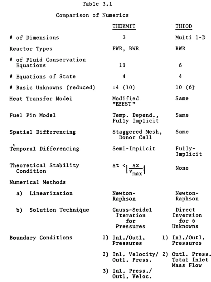
3.3 Comparison of THERMIT and THIOD 75

3.3.1 General Considerations 75

3.3.2 Boundary Conditions 78

3.3.2a Problem Summary 78

3.3.2b Specified Pressure Condition 79

3.3.2c Specified Total Inlet Mass Flow 82 Rate

3.4 Solution Methods 86

3.4.1 Direct Solutica Method 86

3.4.la Solution Principles 86

3.4.1b Encountered Problems 93

3.4.2 Marching Solution Method 98

3.4.2a Solution Principles 98

3.4.2b Advantages of the Marching 100

Methods

3.4.2c Limitations of the Marching 101

3. 5 Summary Methods 106

Chapter 4 NUMERICAL STABILITY ANALYSIS 107

4.1 Introduction 107

4.2 Stability Analysis of THERMIT 108

4.3 Stability Analysis of THIOD 111

4.3.1 General Form of Differential ill

Equations

4.3.2 Local Linear Stability 114

PAGE

4.4 Practical Considerations of Stability 120

and Convergence

4.4.1 Steady State 120

4.4.2 Transients 121

4.5 Summary 122

Chapter 5 THIOD STEADY STATE RESULTS 124

5.1 Introduction 124

5.2 Description of Steady State Solution 125

Scheme

5.3 Single Channel Test Cases 127

5.3.1 Validation of THIOD 127

5.3.2 Steady State Convergence 130

Properties

5.3.3 Sensitivity of Convergence 132

Rate to Constitutive Relations

5.4 Multi-Channel Test Cases 134

5.4.1 Test of Equal Pressure Drop 134

Iteration Option

5.4.2 Comparison of THIOD and THERMIT 139

5,5 Comparison of Solutions and Computational 141 Requirements for Practical One-Dimensional

Cases Using THERMIT and THIOD

5.6 Summary of Results 143

Chapter 6 THIOD TRANSIENT RESULTS 147

6.1 Introduction 147

6.2 Convergence of Solution During Null 149

Transients

6.2.1 Velocity/Pressure Type Boundary 149

Condition

6.2.2 Pressure/Pressure Type Boundary 149

Conditions

6.3.1 Flow Transients

6.3.la Single Phase Flow

6.3.1b Two-Phase Flow

6.3.2 Power Transients

6.3.3 Pressure Transients

6.4 Multi-Channel Test Cases 6.4.1 Flow Transients 6.4.2 Power Transients 6.4.3 Pressure Transient

6.5 Smearing Effect of Step Change in Flow Variables

6.6 Pressure Pulse Propagation

6.7 Comparison of Results and Computational Requirements Using THIOD, THERMIT,

COBRA IIIC/MIT, and an Analytic Solution

6.8 Summary of Results

Chapter 7 REACTIVITY FEEDBACK EFFECTS 7.1 Introduction

7.2 Description of Point Kinetics Model--GAPOTKIN

7.2.1 General Description

7.2.2 Numerical Methods

7.2.3 Test Case

7.3 Coupling of Point Kinetics to THIOD and THERMIT

7.3.1 Time Step Integration

149 150 151 155 157 159 159 166 170 174 178 181 189 191 191 194 194 199 200 202 202

PAGE

7.3.2 Reactivity Coefficients 205

7.3.3 Linear Extrapolation of the 209

Reactivity Function

7.4 Test Cases Using Reactivity Feedback 213

7.4.1 Null Transient 213

7.4.2 Simulated BWR Flow Transient 215

7.4.3 BWR Power Control via Recirculation 221

Flow

7.4.4 Simulated BWR Feedwater Heater Fail- 223

ure Transient

7.4.5 Simulated BWR Pressurization 227

Transient

7.4.6 Simulated BWR Rod Drop Accident 229

7.5 Benchmark Cases 233

7.5.1 SPERT III E-Core Power Transient 233

7.5.la Background 233

7.5.1b Description of Input 234

7.5.lc Calculational Results 238

7.5.2 Peach Bottom-2 Turbine Trip Test 241

7.5.2a Background 241

7.5.2b Description of THIOD Input 243

7.5.2c Results 245

7.6 Summary of Results 251

Chapter 8 253

8.1 Summary of Goals and Methods 253

PAGE

8.3 Feedback to a Point Kinetics 265

Solution

8.4 Recommendations 268

REFERENCES 270

Appendix A Coding Changes to THERMIT and 276

THIOD

A.1 Introduction 276

A.2 Subroutines Added to THIOD 276

A.3 Po.int Kinetics Subroutines Added to 279

THIOD and THERMIT

Appendix B Algebraic Solution of A x = y 281

by Forward Elimination, Backward Substitution

Appendix C Extension of 1-D Marching Method 288

to 3-D

C.1 Introduction 288

C.2 Motivation 288

C.3 Solution Principles 290

C.4 Attempted Solution Strategies 291

C.5 Problems Encountered and 292

LIST OF TABLES

PAGE

1.1 Physical Modeling Advantage of 33

THERMIT over COBRA

1.2 Evolution of Various Computer Codes 35

Leading to an Advanced Transient Analysis Code

2.1 Cases Where One-Dimensional Homo- 40

geneous Equilibrium Theory is Inadequate

3.1 Comparison of Numerics 76

3.2 Comparison of Computational Work 92

Required by THERMIT and THIOD

3.3 Comparison of Computational Require- 102

ments for Direct and Marching Methods of THIOD

5.1 Comparison of THERMIT and THIOD for 129

BWR Fuel Assembly at 4.18 MW and Normal Flow; Steady State Solution

5.2 Effects of Various Thermal-Hydraulic 133

Phenomena on THIOD Steady State Convergence Rate

5.3 Comparison of 4-Channel Calculations 140

Using THERMIT and THIOD

5.4 Computational Requirements of THIOD 144

and THERMIT-for Practical 1-D Test Cases

6.1 Maximum Error in Predicted Core 152

Pressure Drop During Single Phase

Flow Transient

6.2 Maximum Error in Predicted Core 152

Pressure Drop During Single Phase Flow Transient

6.3 Maximum Error in Predicted Values 160

for Single Channel Two-Phase Flow

6.4 Initial Conditions for Multi-Channel 161 Transient Test Cases

6.5 Thermal-Hydraulic Conditions at 3 164

Seconds of Multi-Channel Flow

Transient

6.6 Input for Multi-Channel Power Transient 167

6.7 Input Description for Flow Transient 183

Test Case Comparing THERMIT, -THIOD,

and MEKIN Solutions with Analytic

Results

6.8 Comparison of THIOD and Analytic 184

Solution: Calculated Exit Mass

Flux Error vs. Number of Axial Nodes

6.9 Comparison of THIOD and Analytic 186

Solution: Calculated Exit Mass Flux Error vs. Time Step Size

6.10 Comparison of THERMIT and THIOD 187

Solutions During Flow Transient

6.11 Comparison of THERMIT, THIOD, andMEKIN 188

Results for a 5 Second Period Exp:nenv-tially Decaying Flow Transient

7.1 Test of Point Kinetics Model in THIOD 201

7.2 Maximum Error in Power During Flow 212

Transient with Reactivity Feedback

7.3 Comparison of Predicted Power During 222

Flow Transient

7.4- Predicted Errors During Simulated BWR 230

Feedwater Heater Failure Transient

7.5 Predicted Errors During Pressurization 230

Transient with Reactivity Feedback

7.6 Description of Input for THERMIT - 236

PAGE

7.7 Comparison of Predictions and 240

Experimental Measurements of SPERT-III E-Core Test 86

7.8 Input Description for THIOD Evaluation 246

of Peach Bottom Turbine Trip Test 1

7.9 Summary of THIOD Results for Peach 248

Bottom Turbine Trip Test 1

A.l Subroutines Affected by Conversion of 276

LIST OF FIGURES

PAGE

1.1 Transient Solution Technique 27

of MEKIN

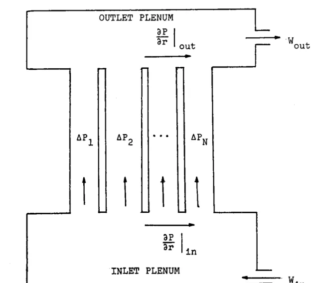
3.1 BWR Core Model in THIOD 81

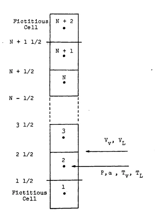
3.2 Axial Noding Scheme 85

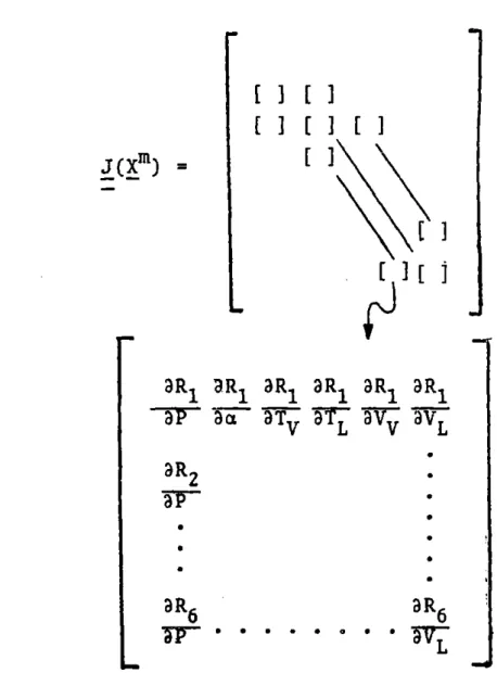
3.3 Structure of Jacobian Supermatrix 88

3.4 Matrix Representation of Algebraic Problem 90

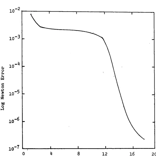
3.5 Log Newton Error vs. Iteration 94

Number for Direct Solution Method

3.6 Log Error in Vapor Velocity vs. 96 Axial Level and Iteration Number

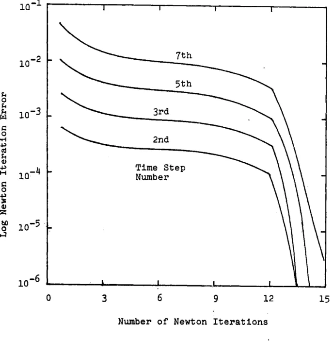
3.7 Log Newton Iteration Error vs. 97

Iteration Number and Time Step for

Power Transient

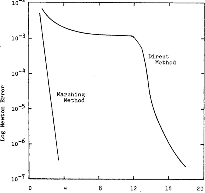
3.8 Rates of Convergence of Direct and 103

Marching Solution Methods for Flow Transient

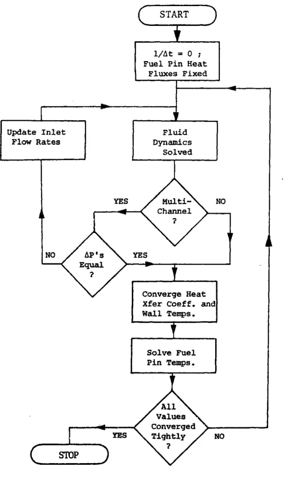
5.1 THIOD Steady-State Solution Scheme 126

5.2 Typical THIOD Steady State Convergence 131

Rates

5.3 Multi-Channel Steady State Convergence 136

Properties

5.4 Multi-Channel BWR Test Case, Assembly 138

Mass Flow Rate vs. Relative Power

5.5 Comparison of Predicted Hot Channel 142

Void Fraction Distribution

6.1 Single Channel Flow Transient Results 153

6.2 Error in Predicted Exit Void Fraction 154

During Single Channel Flow Transient

PAGE

6.4 Single Channel Pressure Transient 158

Results

6.5 Multi-Channel Flow Transient Results 163

6.6 Flow Redistribution During Multi- 165

Channel Flow Transients

6.7 Hot Channel Results for Multi- 168

Channel Power Transient

6.8 Flow Redistribution During Multi- 169

Channel Power Transient

6.9 Multi-Channel Pressure Transient 1.71

Results

6.10 Flow Redistribution During Multi- 173

Channel Pressure Transient

6.11 Input for Transient Test Showing 175

THIOD's Smearing Effect of Flow Variables

6.12 Coolant Thmperature Profile Resulting 176

from Step Change in Inlet Coolant Temperature

6.13 Input for Pressure Pulse Propagation 179

Test Case

6.14 Pressure Profile Resulting from Step 180

Changes in Outlet Pressure

7.1 Spectrum of BWR Transients and 192

Associated Characteristic Times for Change

7.2 THIOD Transient Solution Scheme Using 204

Reactivity Feedback

7.3 Typical Moderator Temperature Coeffi- 206

cient of Reactivity

7.4 Typical BWR Moderator Void Coefficient 207

PAGE

7.5 Typical BWR Doppler Coefficient 208

of Reactivity

7.6 Typical BWR Scram Reactivity Worth 210

7.7 BWR Control Rod Worth During Rod Drop 211

Accident

7.8 Power During Inlet Coolant Temperature 214

Transient

7.9 Null Transient with Reactivity Feedback 216

7.10 Simulated BWR Flow Transient 218

7.11 Maximum Power Error During Flow Tran- 219

sient with Reactivity Feedback

7.12 BWR Operating Map 224

7.13 Simulated BWR Feedwater Heater Failure 226

7.14 Simulated BWR Pressure Transient with 228

Reactivity Feedback

7.15 Power and Reactivities for BWR Rod Drop 232

at Full Power

7.16 SPERT III E-Core Test 86: Experimental 239

and THERMIT Predictions

7.17 Core Inlet and Outlet Boundary Condi- 244

tions for THIOD Analysis of Peach

Bottom Turbine Trip, Test 1

7.18 Peach Bottom Turbine Trip 1 Power 250

History

NOMENCLATURE A C e F g G h n p q

Q

gravitational acceleration mass flux

heat transfer coefficient

reactor power pressure

heat flux

energy source term radius time temperature fluid velocity velocity fluid volume mass flow rate

flow quality

spatial coordinates void (vapor) fraction

effective delayed neutron fraction

rn

2

w

w

kg/sec

A At At AX,AZ p p 1'

precursor decay constant neutron generation time time step size

mesh spacing reactivity density

phase change rate

seC1 sec sec m kg/m3 kg/m3-sec Superscripts m iteration number n old time level n+1 new time level

z axial velocity component

Subscripts

i interface in core inlet

k+1/2 node location in z direction I liquid phase

N greatest node number out core outlet

v vapor phase

Identities Involving SI Units:

1 Pascal = 1 Newton/m2 = 1O-5 bar = 1 kg/m-sec2

Chapter 1 INTRODUCTION

1.1 Overview of Problem

Nuclear reactor safety has continued to be an important issue in recent years. One result of this has been the devel-opment of many large and often complex computer codes used

as tools in understanding the behavior of light-water reactors under transient conditions.

The analysis of certain-transients within the core of a light-water reactor often requires detailed space - and time - dependent modeling to simulate true reactor behavior.

The computer code MEKIN (1) has been developed in an effort

to provide such a "best-estimate" solution. This code couples together 3-D neutronic numerical methods with 3-D thermal-hydraulic (T-H) numerical methods via reactivity feedback

loops.

Figure 1.1 illustrates the sequence of calculations

required for this analysis. Here, the most recently computed thermal-hydraulic state variables (e.g. fuel temperatures,

moderator temperatures, void fractions) are used to generate

updated neutronic parameters. These parameters are then modi-fied to reflect external perturbations (i.e. control rod

motion). The parameters are used to calculate a new neutron flux and precursor distribution via the transient neutronic

EXTERNAL NEUTRONIC PERTURBATION CROS-SECT ION GENERATOR p, T _{, Tm} NEUTRONIC CALCULATIONS

Transient Solution Technique of MEKIN

FISSION and DECAY POWER CALCULATIONS PmP' _c EXTERNAL T-H PERTURBATION TRANSIENT T-H CALCULATIONS Fi gur e 1

calculation. From these fluxes, updated values for the local powers are computed. The thermal-hydraulic boundary conditions are modified to reflect the effect of external perturbations. Then the new set of powers is used to recompute and update

the thermal-hydraulic state variables. This sequence is repeated at successive thermal-hydraulic and neutronic time intervals.

Cook's thesis (2) and the recently completed MIT summary report (3) provide the best summaries of the capabilities and limitations of MEKIN as it now stands in examining both boil-ing-water reactor (BWR) and pressurized-water reactor (PWR) transients. In his investigations with MEKIN, Cook noted that the amount of computing time required for the neutronics portion of the calculations may be as much as 100 times greater than the T-H calculations. Thus, an effort was made to im-prove on the computational efficiency of the neutronic

calcu-lations. The result was the development of QUANDRY (4, 5) a refinement of the Analytic Nodal Method for solving the two-group, multidimensional, static and transient neutron diffu-sion equations. Analysis of many two-and three-dimensional LWR problems have demonstrated that very accurate solutions could be generated with a computational efficiency which is at least two orders of magnitude greater than that of the

conventional finite difference methods used in MEKIN. Hence, there has been increased incentive to improve upon the T-H portion of MEKIN.

1.2 Shortcomings of COBRA IIIC/MIT

The T-H package of MEKIN consists of the subchannel code COBRA IIIC/MIT which computes the flow and enthalpy distribu-tion in nuclear fuel rod bundles and cores for both

steady-state and transient conditions (6,7). In the COBRA code,

the temporal finite difference equations are solved implicitly

by a marching type method. One consequence of this method

is that the axial flow rate must be positive throughout the core. COBRA IIIC/MIT uses a relatively simple homogeneous equilibrium model of the fluid flow in the reactor core. This model assumes that when two-phase flow arises, both liquid and vapor phases travel at the same velocity and that both phases remain at saturation conditions. COBRA IIIC/MIT also uses a simplified crossflow model consisting of transient momentum equations.

A large number of investigations and improvements to the T4H package of MEKIN have been made as noted in Reference

(3). These include comparisons of several heat transfer and

zritical heat flux correlations; the development of a simpli-fied method to include the time dependency of the gap heat transfer coefficient between the fuel pellet and the clad; and a numerical comparison of a MEKIN thermal-hydraulic

transient calculation with an exact analytical solution. The

latter demonstrates the sensitivity of the numerically correct results to a combination of axial mesh size, transient rate

and time step size.

Despite these investigations and improvements to the T-H portion of MEKIN, inherent problems still exists. In their comparison of the computer codes COBRA IIIC/MIT and COBRA IV-I, Kelly et al (8) have indicated some additional shortcomings of COBRA IIIC/MIT in regards to its use in LWR transient analysis. For one, the oversimplified heat trans-fer logic of the code resulted in large discrepenciis in the prediction of clad temperatures when subjected to severe power transients. The code also failed when flow within the reactor was determined to have reversed. This condition may arise during a BWR hot-standby rod drop accident of LWR blowdown for example. Kelly et al also pointed out the questionable use of COBRA IIIC/MIT during blowdown because it employs a pure, homogeneous T-H model. Because of its simplified treatment of transverse momentum, COBRA IIIC/MIT gives crossflow results which are quite sensitive to the selecti6n of axial mesh size.

1.3 Alternate Modeling Approach - THERMIT

In light of these shortcomings of the T-H package

within MEKIN, it is important to note that a somewhat differ-ent approach may offer many advantages over COBRA IIIC/MIT.

The computer code THERMIT (9, 10) has been written with

steady-state and transient, three-dimensional code which employs a two-fluid model to describe two-phase flow and heat transfer dynamics. The code contains a more complete

treatment of the set of conservations equations for momentum transport in all three directions, hence avoiding any of the simplifications in the transverse momentum equations which are common for COBRA IIIC/MIT. The solution method

of THERMIT Allows the treatment of a true boundary value problem by solving the field equations, thus allowing more general pressure boundary conditions to be'handled. The code applies a semi-implicit finite difference scheme which in spite of its greater generality and reliability requires only 50% more computing time than COBRA IIIC/MIT on a per-time-step basis. THERMIT also employs a temperature dependent Uranium heat capacity and thermal conductivity model, and

contains an advanced model for calculation of the fuel-clad gap heat transfer coefficient.

Kelly et al have found that THERMIT in many instances shows better agreement with experimental data than does either COBRA IIIC/MIT or COBRA IV-I. Furthermore, because of its more complete treatment of the conservation of momentum

equa-tions, THERMIT does not show sensitivity to crossflow results with axial mesh size as is the case with COBRA. It is also presumed for this same reason that THERMIT would do much better

These physical modeling differences between COBRA and THERMIT are given in Table 1l..

The three most important differences between COBRA and THERMIT from a numerical viewpoint can be summarized below:

1.

2.

3

THERMIT uses techniques which have a solid base in numerical theory which in most instances will guarantee convergence of the solution, whereas this is not the case with the marching.method of COBRA. Also, THERMIT can treat reverse flow situations.

COBRA cannot handle alternate types of boundary condition other than the imposed inlet flow rate in each channel; THERMIT can handle pressure and flow rate boundary conditions.

COBRA because of its fully implicit finite differ-ence formulation can take very large time steps, while THERMIT is limited by convection.

1.4 Motivation for Improving THERMIT Solution Technique The final point noted above is the only major

dis-advantage facing THERMIT, i.e. THERMIT time step sizes are

limited by the Courant condition:

At < I -- I(1aa1)

Table 1.1

Physical Modeling Advantage of THERMIT over COBRA

1. True 3-D flow equations i.e. no approximation in transverse momentum equations.

2. The two-fluid model allows for:

a) Unequal temperatures of vapor and liquid b) Superheated vapor

c) Superheated liquid

d) Compressibility effects e) Slip between the two phases

f) Countercurrent flow of the two phases

3. Complete boiling curve heat transfer calculations 4. Temperature dependent fuel properties

where AX is the axial mesh spacing and Vmax is the largest fluid velocity. Typically, maximum time step sizes on the order of 80 msec for PWR's and 16 msec for BWR's are allowed. Hence, for steady state calculations THERMIT may require 20

to 40 times as much computing time as COBRA for the same reactor configuration and nodalization, and as much as 15

times for rather mild BWR-type transients. For long transients. or large problems, this time step limitation would be prohibi-tively expensive because of the enormous computing time

required.

Hence, the project reported in this paper focused on the development of a fully implicit, 1-D model for fluid two-phase flow and the application of such a model to LWR trans-inet analysis. The ultimate goal is the implementation of a numerical solution technique which is faster and more accurate than THERMIT for one-dimensional steady state and mild trans-ient cases. Emphasis has been placed on BWR problems. This scheme is especially well-suited to BWR's because of the presence of channel walls which limit transverse flow within the reactor core. In addition, a simple point-kinetics model

has been implemented to investigage the applicability of

two-fluid two-phase models to transients with reactivity

feed-back. The effort in this area is a precursor to a more comprehensive coupling of advanced neutronics and advanced

thermal-hydraulic computer codes. Table 1.2 summarizes the

Evolution of Various Computer Codes Leading

to an Advanced Transient Analysis Code

CODE MEKIN THERMIT qUANDRY THI:OD THERMIT- 2 THERMIT-3 YEAR 1975 1978 1979 1980 1980 1980 Under Devel-opment NEUTRONIC AUTHORS PACKAGE

Bowring et., al.

Reed, Stewart Smith, Greenman, Henry Dube Kelly 3-D Diffusion Theory, Finite Difference None Refined Analytical Nodal Methods Point-Kinetics None Dube, Kelly Griggs (MIT) Point-Kinetics QUANDRY THERMAL-HYDRAULIC PACKAGE COBRA IIC/MIT Advanced Two-Fluid Model Simple Lumped Parameter, No Boiling Fully Implicit, l-D Version of THERMIT Subchannel Version of THERMIT THERMIT-2 THERMIT-2 WA u-'

of developing an advanced LFR transient code.

1.5 Summary of Study

Chapter 2 of this thesis summarizes the various two-fluid, two-phase flow models in the open literature and describes in greater depth the numerical solution scheme used in THERMIT. Chapter 3 explains the development of the one-dimensional, fully implicity version of THERMIT called THIOD (thermal-hydraulic, implicit; one-dimensional), and an explanation'of two attempted solution techniques.

Chapter 4 gives an analysis of the numerical stability of the solution method. Chapters 5 and 6 present steady state and

transient results of THIOD, and comparisons with THERMIT, COBRA, and analytical results. Chapter 7 describes the effect of

reactivity feedback on calculations using both THIOD and THERMIT. Finally, Chapter 8 lists the conclusions of this investigation and makes recommendations for future study.

DESCRIPTION OF TWO-FLUID, TWO-PHASE FLOW MODELS

2.1 Introduction

The past few years have seen the proliferation of computer codas describing two-phase flow phenomena within both light-water reactor and liquid-metal fast breeder reactor cores.

In addition, there has been increased emphasis on the use of systems codes for investigating the response of the pri-mary and secondary reactor systems to a multitude of

opera-tional transients and abnormal occurences.

The COBRA (1,11,12), RELAP (13,14), RETRAN (15), and

TRAC (16) codes are perhaps the most widely used tools for investigating two-phase flow conditions. Each of the codes has been developed and has evolved in response to the need for improved computational efficiency and improved capability to predict reactor systems behavior. It is not the purpose

of this paper to describe in detail all of these codes, and

indeed an excellent summary is provided by Massoud (17). Rather, the objective of this section is to give an overview

of various two-fluid, two-phase flow models and their numerical solution techniques. Particular emphasis is placed on the

code THERMIT which is the basis for most of the work performed in this study. In addition, a review of parallel approaches taken by others to improve the THERMIT (TRAC) solution method is given.

2.2.1 Physical Basis for Two-Fluid Models

The basis for all thermal-hydraulic computer codes is the conservation of fluid mass, momentum, and energy within the nuclear reactor system. Depending on the degree to which one wishes to model the two-phase flow within reactor systems, these models may consist of up to~12 conservation equations in

3 dimensions and 2 or so constitutive equations. The

multi-fluid models we shall consider here are two-multi-fluid, that is, the vapor and liquid phases of a single component such as water. In more sophisticated codes, 3 or more fluids may be considered hence allowing for the treatment of non-conden-sible gases or other fluids. The general principles on which multi-fluid models are based are essentially the same, i.e.

1) Each fluid has associated with it a velocity vector field.

2) Each fluid has an associated temperature field.

3) Each fluid is influenced.by the same pressure field.

4) Each fluid interacts with the other fluids through

interfacial exchange terms.

In the case of water vapor and liquid for example,

evaporation and condensation represent the interfacial mass

exchange term. For two different substances, say water and

nitrogen gas, there is no interfacial mass exchange term. Interfacial momentum exchange represents the loss or gain of

momentum which occurs because of the relative velocities between two fluids. This exchange term usually consists of viscous and drag terms. Interfacial energy exchange repre-sents the flow of heat between two fluids at different temper-atures in addition to energy exchange associated with evapora-tion and condensaevapora-tion.

Hence, two-fluid models (unlike more simple models such as homogeneous-equilibrium) can in theory account for such observed phenomena as thermal nonequilibrium (phases at different temperatures), phase separation, slip flow, and

multi-dimensional effects. These advanced models are required to adequately model the complex phenomena associated with many operational transients and loss-of-coolant accidents. Table

2.1 taken from Reference 18 best summarizes the kinds of events where simple homogeneous equilibrium models are inadequate and where two-fluid models are desirable.

2.2.2 Problems with Two-Fluid Models

The problems associated with fluid modeling are

two-fold:

a) Physical difficulties are encountered when attempts

are made to adequately model the interfacial exchange

terms (mass, momentum, and energy).

b) There are mathematical problems associated with solving che full set of conservation equations.

Table 2.1

Cases Where One-Dimensional Homogeneous Equilibrium Theory is Inadequate (18)

Multidimensional

Effects

Downcomer region Break flow entrance Plena Steam separators Steam generators Reactor Core Nonequilibrium Effects ECC injection Subcooled boiling Post-dryout heat transfer

ECC heat transfer

Low-quality blowdown Reflood quench front

Phase Separation Small breaks Steam generator Horizontal pipe flow Counter current flow PWR ECC Bypass BWR CCFL

2.2.2.a Physical Modeling Problems

Although evaporation, condensation, forced convection, and other physical phenomena are generally well understood for certain cases of two-phase flow, full sets of relations are required to adequately treat the interfacial exchange

terms over the wide range of flow regimes. There is just an insufficient experimental data base on which to formulate an adequate set of relations, and so quite often rather crude simplifications are made.

For examples, in the computer code THERMIT (9), the

interfacial energy exchange term representing heat flow between vapor and liquid is given as

i=hi i(TZ-Tv) (2.1)

where T and Tv are the liquid and vapor temperatures respec-tively, and hi is an equivalent heat transfer coefficient

arbitrarily set equal to 1010 W/m3 - K.

Other simplifications are made by assuming for example that interfacial momentum exchange for three dimensional flow across rod bundles consists of three axial components. Like-wise, in some instances it has been found that interfacial

energy exchange associated with evaporation and condensation

has been completely ignored.

The Electric Power Research Institute realizes this

considerations for improving two-fluid modeling (18).

2.2.2.b Numerical Modeling Problems

The second problem associated with two-fluid modeling can be an even greater one and has been found sometimes to be related to the first problem. The conservation equations

representing fluid flow are usually written as a set of coupled, non-linear, first-order, partial differential equations with non-constant coefficients. Because of this non-linearity and

the complex constitutive relations used, exact solution of the equations is of course impossible. The differential equations are formulated as finite difference equations which themselves are non-linear in nature. Various degrees of implicitness or explicitness are used in an attempt to solve the equations in a numerically stable way.

What is quite often found in practice, however, is that in order to solve these equations the interfacial terms are sometimes oversimplified. Problems sometimes arise because the constitutive packages describing two-phase flow are not mathematically continuous from one flow regime to the next, and the first derivatives are even less so.

Numerical problems arising from the solution of these equations have been known (and experienced by this author)

to lead to conditions of negative void fractions, void

fraction greater than one, or even unreasonable high temperature differences between vapor and liquid.

efforts in two-fluid modeling is the presence of complex characteristics associated with the set of equations (26). For such quasilinear partial differential equations the existence of complex characteristics implies that the

equation set is not well posed and, hence, a small perturb-ation can experience uncontrolled growth. This nonphysical property may be associated with the basic assumption that

both phases are at equal pressure (27). The correction to this problem may actually require the addition of another

conservation equation, and possibly as many as nine (18). Even if the differential equations are well-posed and the treatment of boundary conditions is adequate, the

numerical solution of a coupled set of quasilinear partial differential equations is difficult (28). The flow equations are an extremely stiff set of equations which have a time constant on the order of milliseconds. Numerical evaluation hence usually requires large amounts of computing time or

ignoring high frequency pressure wave history (18).

The largest drawback with two-fluid modeling is the large amount of computing time required to solve the complex set of equations. The problem is compounded not only because

of the increased number of equations associated with the

two-fluid model (10 for 3-D cases compared to 3 for 1-D HEM), but also because of the non-linearity involved with these

Because the difference equations are so complex, it is sometimes quite difficult to formulate the equations in a manner which removes any numerical limitation on the time

step size used. Hence, whereas the HEM model and consequent difference equations used in COBRA IIIC/MIT allows for time step sizes of 0.1, 0.5, 1 sec or even greater, the Courant limit on the time step size for many two-fluid codes may limit this value to 0.02 seconds or even less. It is thus found that along with the increased sophistication and capability of two-fluid modeling comes the tremendous increase in computational requirements. For some rather mild transients, THERMIT for example, may require 15 to 20 times more computing time than does COBRA IIIC/MIT, with often questionable improvement in the accuracy of the results.

2.3 Comparison of Several Two-Fluid Computer Models 2.3.1 TRAC

The Transient Reactor Analysis Code (16, 19) (TRAC) has been developed at the Los Alamos Scientific Laboratory to pro-vide an advanced "best estimate" predictive capability for the

analysis of the postulated accidents in light water reactors. TRAC is the state-of-the-art primary loop analysis code. It employs a three-dimensional two fluid (2 velocities, 2

tempera-tures) model for the primary vessel and a one-dimensional drift

flux model for the rest of the primary loop. A cylindrical

vessel. Development of the TRAC computer code was the first major effort to put all of the required

loss-of-coolant-accident (LOCA) models into a single, advanced, best estimate code. It features two-phase nonequilibrium hydrodynamics

models; flow-regime-dependent constititive equation treatment; reflood tracking capability for both bottom flood and falling film quench fronts; and consistent treatment of entire accident sequences including the generation of consistent initial

conditions.

The fluid dynamics methods are of course of greatest

interest in this report. The TRAC method employs the full six equation set of conservation equations, i.e. conservation of mass, momentum, and energy for vapor and liquid. Because of the three dimensional treatment there are actually 10 scalar equations and 10 unknowns for each fluid cell within the core. Finite difference approximations are used to convert these partial differential equations into a set of linear algebraic

equations that can be solved on a computer. Liles and Raed (20) were the first to develop the numerical solution strategy for

solving these equations although recent improvements have been made as will be mentioned later in this chapter.

It is well known that the set of field equations described by the six partial differential equations have complex

character-istics which represent a partially elliptic system. So long as the mesh size is not too small and the interfacial momentum

numerically (20,21). In the staggered difference scheme (22) as employed in TRAC, the velocities are located on

the mesh cell surfaces while the volume properties of pressure void fraction, fluid temperatures, fluid densities, fluid

enthalpies and so forth are located at the mesh-cell centers. The scalar field equations (mass and energy) are written over a given mesh cell while the momentum equations are staggered between mesh cells in the three component directions.

The finite difference equations are written semi-impli-citly, that is, with some of the variables defined at the old time step and some at the new time step. The donor-cell averaged or upwind differencing method provides stability to this partially implicit method. This method is similar to the well-known ICE technique (22), but includes a more implicit coupling of energy equations to mass and momentum equations.

The differenced equations are linearized and solved by

Gauss-Seidel iteration. A Gauss-Seidel iteration procedure is also used to handle coupling between one-dimensional

compon-ents of the model.

The result of the numerical methods employed in TRAC is a stability limit on the allowed time step used, governed by material convection (i.e. the Courant limit). For typical LOCA conditions this limit can mean restriction to time step sizes of I ms or less, and prohibitively high computation

The finite-difference scheme described above for the most part works quite well. However, there are limitations as regards numerical diffusion (23) and a phenomenon often called "water packing'.'(24). Also, since it is a first-order method in space (and time) it requires a large number of mesh cells to model large gradients adequately. Again, this leads to long problem execution times.

2.3.2 COBRA-TF

Like its cousins, the COBRA-TF code (12,25) was developed at Battelle-Northwest Laboratories. In 1978 EPRI sponsored the development of COBRA-TF (EPRI) as a streamlined, fast-running, two-fluid code designed by C. W. Stewart specifically to simulate thermal-hydraulic behavior of PWR steam generators. This code used X COBRA (which may eventually be released as COBRA-V) as a basis, to which a simplified 6-equation two-fluid model adapted from COBRA-TF was added.

The COBRA-TF code itself is a two-fluid, three-field thermal-hydraulic model being developed for best estimate safety analysis of light water reactors. Its specific appli-cation is for hot bundle analysis and analysis of Upper Head Injection System equipped PWRs.

In this code, entrained liqdid can be treated as a

separate field, It thus has a velocity field which is quite

different from the continuous liquid field. This essential

feature is important for correctly modeling reflood

used to perform some reflood simulations of FLECHT data. COBRA-TF was originally developed as a subchannel code, but the momentum equations have been extended to model full three-dimensional flow. The code has been generalized to allow the nodalization of the entire reactor vessel and its internals. Additionally, COBRA-TF has been implemented into TRAC as the vessel module by the Pacific Northwest

Laboratories. The COBRA/TRAC code is being used to simulate Semiscale Mod 3 and FLECHT reflood tests.

The main differences between COBRA-TF and the 3D

component of TRAC is that COBRA-TF does allow for the three-field formulation. COBRA-TF uses Cartesian coordinates as opposed to cylindrical coordinates. In addition, COBRA-TF employs a generalized nodalization scheme which allows for variable noding and the modeling of complex reactor internals. The numerical solution scheme (with the exception of the

additional field for entrained liquid) is essentially identi-cal to that developed at LASL. Since more equations are

involved, COBRA-TF is naturally slightly more complex. The COBRA-TF noding flexibility does allow the code to model BWR cores and recirculation loops. Presently, the BWR

version of TRAC is being developed by Idaho National

2.3.3 VENUS-III

The Venus-III techniques (29) were developed for solving multi-component, two-dimensional thermal-hydraulic-neutronic

problems which arise in the analysis of hypothetical core disruptive accidents in LMFBRs. The first algorithm however

treats the system with a homogeneous flow assumption where a multi-component pressure "Poisson" equation is developed, and hence is of no concern to us here. The second algorithm treats the system using a two fluid model and implicitly solves the separate fluid mass and momentum equations using a two-level iteration strategy. The energy equations are

partially decoupled and the quasi-implicit temperature

algorithm used in the homogeneous flow analysis is employed. The algorithm thus basically consists of the simultaneous

solution of the non-linear coupled difference equations for

component mass and momentum conservation. Mixture mass and

momentum equations are used and relative velocities describe the movement of individual components through the field.

To solve the coupled equations, one notes that the local variables such as pressure and velocity are coupled to

neighboring cell variables through a set of non-linear alge-braic equations. This then defines the two-level solution

sweep across the mesh in a Gauss-Seidel fashion, using up-dated variables as they are generated in the solution. Thus, within each cell, assuming a knowledge of surrounding cell variables through their present Gauss-Seidel iterate, the local non-linear algebraic set of equations is solved for using a multi-variate Newton-Raphson technique. The solution then marches through the nodes, stopping at each node to

calculate the algebraic equation solution, and then marching to the next cell, while updating the iterates at the neigh-boring cells. Two levels of iteration are employed since the Newton-Raphson solution is used.

The technique described above is quite complex when

compared to the homogeneous flow approach and is computation-ally more expensive. The method also is not unconditionally

stable, although an extension of the method for one-dimensional gas systems is apparently unconditionally stable (29,30).

The application of the VENUS-III method is to

dis-assembly analysis of sodium cooled fast reactors. The primary field components are the fuel and structure, while the

secondary field is chosen as the sodium coolant. Neutronic effects are included through motion feedback of the fue material motion, which is generally negative, and through

sodium voiding which is generally positive.

The modeling and solution methods employed are different

which is the assumption in VENUS-III of thermal equilibrium of two-phase systems. Additionally, the VENUS-III method

is restricted to two dimensions in cylindrical coordinates (r, z). An Eularian hydrodynamics formulation similar to TRAC and COBRA-TF is employed.

2.4 Descri2tionof THERMIT

2.4.1 Overview of Modeling

The THERMIT computer code (9,10,31,3_2) calculates the three-dimensional transient thermal hydraulic behavior of light water reactor cores. THERMIT offers advances in both the physical and numerical aspects of T-H analysis. The code solves transient compressible fluid flow equations for both single-phase and:two-phase flow in the rectangular geometry of the reactor core, simultaneously coupled with a fuel rod

heat conduction model via a best estimate heat transfer package. THERMIT was intended to analyze core-wide thermal-hydraulic

behavior during space-dependent transients using fluid flow control volumes whose transverse dimensions are roughly the size of an assembly. However, recent improvements have

extended THERMIT's application to subchannel analysis as well (10,32).

The three main criteria on which the code is based can

1) The code solves the full multi-dimensional

conser-vation equations.

2) The numerical solution technique does not rely on any assumption about the direction of flow.

3) The numerical method is both reliable and efficient, and the convergence and stability properties have a

sound mathematical basis.

Hence, the solution scheme used is a semi-implicit finite difference method for the fluid dynamics based on the three-dimensional pressure field scheme developed for TRAC. The basic difference is that THERMIT treats Cartesian coordinates as opposed to cylindrical coordinates. The code includes some physical models which are new to LWR core flow analysis. For example, interbundle crossflow is determined by the net effect of pressure gradients, inertia, and friction laws describing resistance to transverse flow through tube banks.

Two-fluid conservation equations (as with TRAC and other codes) are used to describe the two-phase flow. Vapor and liquid are treated as the two fluids. These equations are very general and limited only by the choice of the interfacial exchange terms. Both PWR and BWR cores can be modeled and analyzed under steady state and transient conditions.

The two-fluid equations are solved in first-order finite

The result is a numerical stability restriction in the form

of a maximum allowable time step:

At < AX/V (2.2)

where AX is the mesh size and V is the larger of the vapor and liquid velocities. At each time step, the equations are

solved with a Newton iteration method which reduces the system of equations to a simplified boundary value problem for

pressures only. Convergence can be obtained by choosing

sufficiently small enough time steps even for the most severe

of transients.

The primary application for which THERMIT was developed is the eventual inclusion in a transient multidimensional

reactor kinetics code with thermal hydraulic feedback. Because of the sensitivity of feedback to moderator density, and be-cause THERMIT represents state-of-the-art thermal-hydraulics,

the code offers the best potential for meeting analytical needs.

2.4.2 Fluid Dynamics Equations 2.4.2a Conservation Equations

The fluid dynamic algorithms of THERMIT are based on a set of six basic conservation equations for mass, momentum and energy of each phase of the fluid. These equations are formulated under the assumption that each phase behaves as a

separate fluid under the action of a common pressure field, with the simple additional constraint that the two fluids must share the available volume. This constraint is

imposed by defining a void fraction a (more properly called the vapor volume fraction). The void fraction is defined

by requiring for some control volume AV that aAV be the

volume occupied by the vapor. The two-fluid equations are written in terms of a and the microscopic phase densities

Pv and p. These densities represent the true thermodynamic

densities of the phases obtained from the equations of state. The conservation equations on which THERMIT is based

are as follows (9):

Conservation of Vapor Mass

it (apV) + V. (apv vC) =

r

Conservation of Liquid Mass (2.4)

aJ

'5t (1-cYOP] + V - [(-a) pV =

-r

Conservation of Vapor Momentum (2.5)

Conservation of Liquid Momentum (2.6)

a

= -W + - (1-c) Pz

Conservation of Vapor Energy (2.7)

a (apev) + V'(ap e vv) (t+vPv- v) + P at Q + Q

Conservation of Liquid Energx (2.8)

[(1-a) p e] + V-f(l-cz) p e V9] + P V-[(l-ci%]

S~E = 9wt -Qi

(See Nomenclature Table on Page 22)

The momentum equations above are vector equations in 3-D and scalar equations in 1-D-. Because these equations are quite complicated and for reasons involved w-ith the selection of a difference strategy for solving these equations, they

were rewritten in a non-conservative form. This is accomplished by differentiating by parts. the first two terms of Eqs. (2.5)

and (2.6) and by using the mass equations to simplify expression. This process yields the following equations (9):

(2.9') (1-a)pz av + (l-a)p

(YVz-V)Vz

-

P

P

where the non-conservative momentum equation exchange terms iv and

P

V.=f + r V"' (2.11a)

P.

=4-.

-Iiy

(2.11k)

It should be noted that, for this non-conservative form of the momentum equations, it is no longer necessary that the exchange terms be equal in magnitude and of opposite sign.

In fact, the above equations shu;a this will not be true unless vv = v or unless r = 0.

2.4.2b Additional Relations

In addition to these conservation equations there are four equations of state, i.e.

PV = V (P, TV) (2.12)

P- P (P, Tt) (2.13)

(2.14)

e

-e

Cg

e.= e. (P, Tz) (2.15)

Altogether there are ten conservation equations (2 mass, 2 energy, 6 momentum) in 3 dimensions and four equations of state, givifng a total of fourteen equations. The fourteen unknown variables are the pressure P, the void fraction a, the densities, pV and p., the internal energies, ev and e., the temperatures, TV and Tz, and the three components of the velocity vectors, ,Y and V.

In addition, the constitutive relations include the inter-facial exchange terms. The vapor-liquid interaction terms

are the vapor production rate, r, the interfacial momentum exchange rates, F. and F it and the interfacial heat

trans-iv

fer rate,

Qi.

Qwv

Qwz,

Fwv and FwZ. Models for each of these constitutive relations are either empirically or semi-empirically based (9,10,32).

2.4.2.c Fiiite Difference Equations

The above differential equations are discretized in space and time to obtain a set of non-linear algebraic

equations for all unknowns. When combined with the equations of state for internal energy and density of vapor and liquid,

the result is fourteen equations and fourteen unknowns in three dimensions.

For simplicity and an easier comparison with the differ-encing scheme chosen and described later, the difference

equations in one dimension (axial) as employed by THERMIT are given below (9):

Vapor Mass

n+l

-(apv) - (apV) n+1 [A(ap )n v )n+1k(2.16)

At {[AVaIn( ) lk+l/2

- [A(ap ) n(Vz) n+l = n+1/2

V V Ik-1/2 r

Liquid Mass

Same as Eq. (2.16) with a replaced by (1 - a), sub-script v by k and r by -r. Vapor Energy (apeV)nl-(apeV)4 _{1 pn + n} (2.17) At+ [ (pe)v]27k+1/21 An vz )n+1 [Aa(v) _k+1/2 -1[Pn + (P e) k- /2 [Aa (v)n+ k-/2 n a n+1 _a n

Qn+1/2

+Q

Liquid Energy

Same as Eq. (2.17) with a replaced by (1 - a), subscript v replaced by , and

Qi

TFv

Same as Eq. (2.18) with a replaced by (1- a), subscript v replaced by 1, and -Fiv by + F.

In the above expressions, donor cell differencing is used for describing the properties which are evaluated at the

faces of the mesh cell in the mass energy equations. Let C stand for any cell-centered quantity such as a, P, p, pz, etc. Then the value of Ck+1/2 is determined as

(2ol9)

Ck+l

if (Vz)k+1/2< 0

_if(Vz)

In ths momentum equations, such properties are obtained by using spatially weighted averages as shown below:

CkAzk + Ck+l Azk+l (2.20)

Ck+1/2 = _{Azk+ Azk+l}

In addition, the convective derivative in the momentum equation iA given by:

K4+3/2 V~k+1/2 . A v z AYk+3 2 4 if(v k+1/2 < 0 k+1/2a k 2k-/2 if (Vv)k+1/2 _{> 0} Az k (2.21)

Finally, (Az)k+1/2 is defined by:

("4k+1/2 (Az)k + (Az)k+l (2.22)

Note that in the above expressions, some of the terms in the difference equations are evaluated at the old time step n, some at the new time step n+l, and some terms (the

exchange terms in particular) are evaluated using both old and new time values, i.e. n+1/2. Note also that the equations are differenced spatially on a staggered mesh.