An interactive chemical dynamical radiative two-dimensional model of the middle atmosphere

HAL Id: insu-02793804

https://hal-insu.archives-ouvertes.fr/insu-02793804

Submitted on 5 Jun 2020

HAL is a multi-disciplinary open access

archive for the deposit and dissemination of

sci-entific research documents, whether they are

pub-lished or not. The documents may come from

teaching and research institutions in France or

abroad, or from public or private research centers.

L’archive ouverte pluridisciplinaire HAL, est

destinée au dépôt et à la diffusion de documents

scientifiques de niveau recherche, publiés ou non,

émanant des établissements d’enseignement et de

recherche français ou étrangers, des laboratoires

publics ou privés.

An interactive chemical dynamical radiative

two-dimensional model of the middle atmosphere

G. Brasseur, M.H. Hitchman, S. Walters, M. Dymek, Michel Pirre

To cite this version:

G. Brasseur, M.H. Hitchman, S. Walters, M. Dymek, Michel Pirre. An interactive chemical dynamical

radiative two-dimensional model of the middle atmosphere. Journal of Geophysical Research,

Ameri-can Geophysical Union, 1990, 95 (D5), pp.5639-5655. �10.1029/JD095iD05p05639�. �insu-02793804�

JOURNAL OF GEOPHYSICAL RESEARCH, VOL. 95, NO. D5, PAGES 5639-5655, APRIL 20, 1990

An Interactive Chemical Dynamical Radiative Two-Dimensional Model

of the Middle Atmosphere

G. BRASSEUR,

1 M. H. HITCHMAN,

2 S. WALTERS,

1 M. DYMEK,

3 E. FALISE,

3 AND

M. PIRRE

4

This paper describes a new two-dimensional model of the stratosphere and the mesosphere in which dynamics, radiation and chemistry axe treated interactively. The transport equations axe expressed in the transformed Eulerian fraxnework. Momentum deposition associated with Rossby wave absorption and gravity wave breaking and related eddy diffusion coefficients are paxaxneterized as a function of the mean zonal state of the atmosphere. Diabatic heating and cooling is derived from the detailed National Center for Atmospheric Reseaxch community climate model radiative code. The distributions of chemically active species belonging to the oxygen, hydrogen, nitrogen and chlorine families axe calculated for present-day conditions. By applying neax the tropopause a different dynamical forcing in each hemisphere, the model produces

significant hemispheric asymmetries in dynamical quantities (e.g., temperature) and trace gas densities (e.g., column ozone), in good agreement with climatological values. It is shown that the

calculated distributions of source gases, such as nitrous oxide and methane, axe very sensitive to the

calculated (and pararneterized) dynamical quantities and that species produced in the atmosphere,

like carbon monoxide and odd nitrogen, can provide interesting information on the role of atmospheric transport. A major problem that remains to be elucidated is the underestimation by most models of the ozone density in the upper stratosphere. Because of the many feedback mechaaftsms included in its formulation, the model is well adapted to study the effects of human or natural perturbations. The response of the atmosphere to perturbations resulting from increasing emissions of CO2 and chlorofluorocaxbons is considered.

1. INTRODUCTION

Two-dimensional chemical transport models have been extensively developed in the last 2 decades to study the behavior, as a function of latitude and height, of atmo- spheric trace species. These models provide useful in- formation on the zonally averaged distribution and the• sources and sinks as well as the meridional transport of these chemically active constituents. One advantage of

two-dimensional formulations over one-dimensional mod-

els is their ability to represent the effects of dynamics in redistributing constituents in the meridional plane. A difficult problem, however, in representing zonally aver- aged distributions arises from the nature of stratospheric transport, which is due in large part to planetary waves and is thus three-dimensional by essence. In the so-called Eulerian models, the mass and energy fluxes are sepa- rated into a component involving the zonally averaged meridional winds and a component associated with the eddies, i.e., the departure of the variables from their zonal mean. The contribution by the eddies requires additional information through a closure relation by which the eddy transport of quasi-conservative tracer is specified in terms

of the gradient of their mixing ratios (based on hnear

theory assumptions). In the two-dimensional models of

the first generation, the mean circulation is prescribed, and the mixing coefficients are specified and are based on a mixing length hypothesis; their values are generally obtained from studies on the dispersion of nuclear debris

iNational

Center

for Atmospheric

Research,

Boulder,

2Depaxtment of Meteorology, University of Wisconsin,

Madison.

3Belgian Institute for Space Aeronomy, Brussels.

4Laboratoire de Physique et Chimie de l'Environnement,

Orl6ans, France.

Copyright 1990 by the American Geophysical Union.

Paper number 89JD02868.

0148-0227 / 90 / 89 JD-02868505.00

[Reed

and German, 1965; Gudiksen

et al., 1968]. According

to the noninteraction

and nontransport

theorems

(see, for

example, Andrews

et al., [1987] for a discussion),

however,

the transport by the Eulerian mean kirculation and by

the large-scale

eddies nearly cancel, so that inaccuracies

in the specified diffusivities lead to •ignificant errors in

the determination of the net transport.

The assumption that eddy transport can be properly modeled by a simple diffusion law was questioned, for

example, by Mahlraan [1975], who found from a gen-

eral circulation model (GCM) study that the eddy flux

is not always diffusive in nature and that some of the

assumptions

made by Reed and German [1965] regarding

the conservative nature of the species, the particle tra- jectory and the mean slope of the mixing surfaces are dubious. Solving the eddy perturbation equations with

the linear wave approximation,

it was found (see, for ex-

ample, Plumb [1979], Pyle and Rogers [1980b], Matsuno

[1980]) that the flux-gradient

relation suggested

by Reed

and German can be retained but that the eddy tensor can be separated into a symmetric and an antisymmetric component. The latter, advective in character, depends on the mean parcel displacement and, if combined with the mean meridional circulation, provides an effective trans- port circulation. The former, which is a dispersive com- ponent, is determined by the time variation of the parcel

displacement

(transient eddies) and by the photochemical

relaxation rate (chemical

eddies). Dunkerton

[1978] sug-

gested that the transformed

Eulerian mean (TEM) circu-

lation (residual

circulation)

(•*, W*) defined

by Andrews

and Mcintyre [1976] and Boyd [1976]

5639

5640 BRASSEUR ET AL.: INTERACTIVE MODEL OF THE MIDDLE ATMOSPHERE

where (•, W) represents

the Eulerian mean (EM) circula-

tion (see the notation

section

for other definitions)

would

by Brewer [1949], Dobson

[1956], and Murgatroyd

and Sin-

gleton [1961] and to the Lagrangian mean circulation of

air parcels. In the two-dimensional models developed fol-

lowing the TEM theory, based on a global advective trans- port circulation [e.g., Garcia and Solomon, 1983; Guthrie et al., 1984; Stordal, 1985], eddy diffusivities were nev- ertheless added in the thermodynamic and trace species continuity equations to account for transient and dissipa- tive processes which are expected to become important especially in winter. The magnitude of the eddy diffusivi- ties required by these models is approximately an order of magnitude smaller than in the classical Eulerian models. In this formulation, the values of the eddy diffusivity are usually specified empirically, and the relationships among dissipation mechanisms, the distribution of wave absorp- tion, and irreversible mixing are therefore ignored. In the most recent models however, these processes are deter-

mined in a consistent manner.

The purpose of this paper is to describe a two-

dimensional model formulated in transformed Eulerian co-

ordinates, in which chemical, radiative, and dynamical processes are treated interactively, and to present results obtained regarding the present-day and the perturbed at- mosphere. The model includes a detailed radiative scheme which derives the diabatic heating rates consistently with calculated distributions of temperature and trace species densities. Calculated wave driving and eddy mixing coeffi- cients resulting from gravity and Rossby wave absorption vary with the evolving distribution of the mean zonal wind. Through the large number of interactive processes included, the model is particularly adapted to the study

of feedback mechanisms regulating the middle atmosphere

when natural or man-made perturbations are produced.

2. MODEL DESCRIPTION

œ.1. Dynamics

The model, which is used in the present

study, extends

from pole to pole with a latitudinal resolution of 5 o and from the surface to 85 km with a vertical resolution of I km. The potential temperature and the chemical species are advected by the transformed Eulerian mean

meridional

circulation

in log-pressure

coordinates,

which is

forced

by spatial

gradients

in wave

driving

and the related

net radiative

heating.

The dynamical

fields

(•, •*, •*, 0)

are obtained

from the thermodynamic,

zonal momentum,

00 •. •0

•0 --

O--•+

•-• +•*•z = Q + D8

(1)

O

t rt

•* q-

•zz

w -- F

(2)

•--(•*

cos

4) + • 0

_{••(•o•*)}

=o

• = -• o-•

(4)

1 0 (7 cos

4)

(5)

cos

• Oy

is the absolute vorticity and where tan•b

7 = f q- 27

(6)

The other variables are defined in the notation section.

The eddy heat flux divergence D0 expressed by

= - o-T

• Oo

w,S,

+ o•/oz

•,o,

(•)

is generally small except where transience and dissipation is important, for example, in the mesosphere, where gravity wave breaking can cause a substantial downward heat flux. The wave driving F is assumed to be due to

Rossby

(FR) and gravity (Fg) wave dissipation,

which can

be expressed

by the divergence

of wave activity flux (or

Eliassen-Palm

(EP) flux E)

1

•=•n+ • = oo

• cos

4, v.r

(s)

where the meridional and vertical components of E are

Ey

=

po

a

cosqS

[ O•'/Oz

v'O'

--

u'v']

(9a)

M/Oz - .,w,

(9•)

Equations

(1) to (4) can be combined

to give a diagnostic

equation for the mean meridional stream function [Garcia and Solomon, 1983]

%Y•j•

+%• OyOz ••+%•+c,•

= c• cos

•

(10)

where the •velocity" stream function X •nd the "m•ss" stream functions • •re related to the components of the mean meridionM velocity by

_.

v ...

•

o (OoX)

-

•

(11a)

po cos 40z po cos 40z

_.

w ....

•

o (ooX) •

(11b)

po cos 40y po cos 40y

the equation coefficients

(Cry, %•, O•, %, ana O•)

are functions of the mean zonal wind and temperature

distributions [Garcia and Solomon, 1983], and the forcing

term (7 F is a function of the meridional gradient of the heating rate and the vertical gradient of the momentum torque associated with wave breaking:

R 0 --

fOF

C•,

= • •yy(Q

- Do)

+ •

(12)

Given the forcing term (to be described

shortly), previous

values

of 0 (or T) and 7, and the boundary

conditions

(X

= 0 at the poles, Ox/Oz = 0 at the top and a specified

BRASSEUR ET AL.: INTERACTIVE MODEL or THE MIDDLE ATMOSPHERE 5641 90N 6O 3O EQ 30 60 w" (mm/s) 15 km - [ [ ] / ] Ii [ [ [/ [ [ I • [ •[ • • I [ • [ [ [ 1 - i I I x - -0.:32 -0.:32 \ \ -

Z /I /I //

\• • \\ \ •

-

Aside from the influence of the 15-km boundary con- dition, the dynamical system is kept from radiative equi-

librium conditions

(7* - •* - 0; • - 0) through

momen-

The contribution of gravity waves is parameterized by the scheme proposed by Lindzen [1981] and Holton

[1982] and adopted by Garcia and Solomon [1985]. In

this scheme, zonally traveling waves break when their

90S-' ' ,, i I • •, •, !,,,

] • I • [ t [ t I-

amplitudes

become

so large

that they become

convectively

12/23 3/18 6/17 9/20 12/18 unstable. Momentum deposition above the breaking level

DATE

tends to accelerate (or decelerate) the zonal wind speed

• toward the zonal phase speed c of the wave. In the

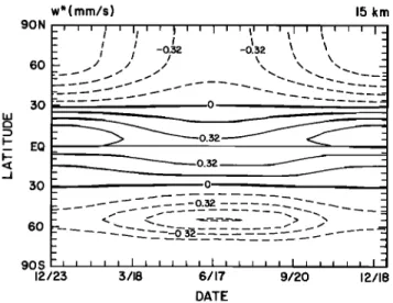
Fig. 1. Transformed

Eulerian

mean

vertical

velocity

(in millime- region

between

the breaking

level

zb and the critical

level

ters

per

second)

specified

at iS-kin

altitude

(tropospheric

forc- (where

•

c) wave

amplitudes

are

assumed

to cease

ing),

as a function

of latitude

and season.

Contour

interval:

0.16 zc

--

,

mm/s.

their exponential

growth

with altitude and are reduced

classical alternating direction method and provides the

transformed Eulerian mean meridional circulation.

For the calculations of the dynamical quantities, the lower boundary is located at 15-km altitude where the

to a constant profile by convective turbulence. The body

force transferred from the waves to the local mean flow

is given by

(13)

vertical

velocity

is specified

as shown

in Figure

1. (This in the range

zb < z < ze, where

the breaking

level is

condition,

which simulates

the dynamical

forcing

from determined

by

the troposphere, is equivalent to a specified value of the

stream

function

X.)

Below

15

km,

where

the

formulation

of

mass

and

energy

transport

by

the

residual

circulation zb

= 3H

In [c-•[

(14)

is not straightforward because of the large transient

and dissipative effects, the stream function is specified and where H is the scale height. Parameters B and •,

as a "return flow" to close up the two stratospheric which represent

wave properties at 15 km (see, for exam-

meridional

cells. Sensitivity calculations

have shown that ple, Brasseur

and Hitchman [1987]) are specified

in Table

the structure of the temperature field as well as the I for the spectrum of phase speeds used in the present

slope of the mixing ratio isolines of the tracers in the study. The values of these parameters have been adjusted lower stratosphere is very sensitive to the strength of to make the calculated body force consistent with the

the circulation specified at 15 km. For example, the momentum budget of the middle atmosphere established

temperature minimum at the tropical tropopause changes for mid-December 1978 from the limb infrared monitor

by about 10 K if the wind velocity at the tropopause

is of the stratosphere

(LIMS) observations

[Hitchman and

modified by 50%. Therefore we have tuned the values Leovy, 1986]. The algorithm then was applied at all times. of the wind condition in order to obtain a temperature According to the parameterization of Lindzen, the verti-

distribution in fair agreement with climatological values. cal eddy diffusion coefficient associated with gravity wave

This forcing varies with season and is different in each breaking above the zb level is given by

hemisphere. It should be noted that the use of a

fixed

_"frozen"

dynamical

_circulation

boundary

_and

_temperature

condition

at 15

_below

km

_this

and

_level

a

IYzz

_--•'•

B (6_•)3

(c_•)_{_3H•z

z

reduces

the consistency

of the model and limits the Profiles

of Fg and IYzz are smoothed

in the vertical

accuracy

of calculated

ozone perturbations

in response to avoid numerical

problems

when solving

the transport

resolved, since the circulation in the lower stratosphere is driven by the wave forcing in the troposphere, a quantity that cannot be accurately estimated, especially in a two-dimensional model. Perhaps a way to improve the dynamical formulation in the lower stratosphere, with

consistent

mean circulation and wave driving (see below),

is to determine both vertical velocity and wave activity in the troposphere from zonal mean climatological fields. At the present stage of the model development, an empirical

wind condition determined to fit the observed ozone

column and the temperature seems more appropriate.

TABLE 1. Parameters Adopted for the Calculation of

Wave Drag and Eddy Diffusion Associated with

Gravity Wave Breaking

c, m/s B, 10-9s/m 2 •, m/s -40 0.5 3.0 -20 1.0 3.0 0 2.0 3.0 +20 1.0 3.0 +40 0.5 3.0

5642 BRASSEUR ET AL.: INTERACTIVE MODEL OF THE MIDDLE ATMOSPHERE

equations.

A background

value

of 0.1 m2/s is added

and accounts for all additional processes not included in

Lindzen's formulation.

To determine the momentum deposition

rate as well as

eddy coefficients

associated

with planetary

wave

breaking,

an equation

for Rossby

wave activity is added to the

system.

According

to Edmon

et al. [1980]

and Hitchman

and Brasseur

[1988],

Rossby

wave

activity

A is conserved

following

the WKBJ group velocity

(7 unless

there are

OA 1 O

₊

_oy

₊

O (GzA)--c•A (16)

This equation can be solved provided that the merid-

ional and vertical components

of the group velocity (Gy

and Gz) as well as the wave damping rate a are known

and that proper boundary conditions are specified. Hitch-

man and Brasseur [1988], using the dispersion

relation for

quasi-stationary undamped waves on the beta plane, have

derived an expression for the group velocity components as a function of the mean zonal state of the atmosphere. Given a source of wave activity at 15-km altitude, based on climatological values and accounting for the tropo- spheric forcing of the planetary waves, and using a damp- ing rate

c•(z)=0.7+0.6

tanh[(Z(k•)•

-50)]

day_•

intended to represent the effects of radiative and mechan-

ical damping on Rossby waves, equation (16) is solved

through an alternating direction method. The upper boundary condition is A = 0, while OA/Oy = 0 is spec- ified at the poles. The components of the Eliassen-Palm flux, from which the body force can easily be calculated, are then given by the simple linear wave approximation

[Hitchman and Brasseur, 1988]

=

œ• =G•A

(17b)

Since for quasi-geostrophic Rossby waves, the meridional

flux of eddy potential vorticity (vtq

t) is proportional to

the divergence of the quasi-geostrophic EP flux lEdmort

et al., 1980], the mixing coefficient for potential vorticity

(q) can be derived from the following expression

V.E

Kyy

-- - poacosc)O•/Oy (lS)

Thus in this formulation the dissipative processes respon- sible for wave driving are also responsible for irreversible mixing of potential vorticity. As discussed by Hitchman

and Brasscur

[19881,

the vMues of Kyy derived from (lS)

for potential vorticity are generally applicable to chemi- cMly active tracers. If the lifetime of the tracer is similar to that of potentiM vorticity or if mechanicM dissipation dominates, Kyy can be used for the tracer. If the tracer concentration is photochemicaHy controlled, the behavior

of the species is insensitive to the value of Kyy. If Rossby

wave activity is primarily radiatively damped and if simul- taneously the tracer •fetime is much larger than that for potential vorticity, then other values of Kyy should be

determined for the tracer. In this study we assume that

Kyy and Kzz derived

from the formulations

described

in

this paper apply to all variables.

The temperature

distribution

is derived

from the ther-

modynamic

equation

(1) in which the contribution

of the

small-scale

eddies

(Do) is assumed

to be related

to verti-

cal eddy exchanges,

so that Do is parameterized

by

Do=

1

0

[ 0•] (19)

where Kzz includes the diffusivity associated

with gravity

wave breaking.

œ.œ. Radiation

The net diabatic heating rate Q is calculated from

the detailed radiative code used in the latest version of

the National Center for Atmospheric

Research

(NCAR)

community

climate model (CCM1)[Kiehl et al., 1987].

by several

trace gases: the contribution

of ozone

in the

Hansen [1974], the effect of water vapor in the near-

and Cess

[1985]

for the direct beam and the formulation

of Lacis and Hansen

[1974]

for the reflected

beam, and the

effect of carbon dioxide in the near-infrared is calculated

from the formulation of Sasamori et al. [1972]; finally,

the contribution of molecular oxygen in the near-infrared

is determined from the parameterization of Kiehl and

Yamanouchi

[1985]. The radiative transfer equation is

solved for two large spectral regions: 0-0.9 #m and 0.9-

4.0 #m, respectively. The 24-hour average of the solar

heating is calculated

consistently

with the method used

to derive the 24 hour average of the photodissociation coefficients. In the present version of the model, the

effect of clouds is ignored, and the surface albedo at all

wavelengths

is taken to be 0.1. The ground temperature

is specified

by climatological

values. However, since the

dynamics in the model is calculated interactively only

above the tropopause, the temperature calculated below 10 km is replaced by climatological values compiled by

Randel [1987]. A hnear interpolation

between

calculated

and climatological values is performed between 10 and

The integration of the thermodynamic

equation, which

provides the distribution of the zonally averaged temper-

ature, is spht into two successive

steps and performed by

an alternating direction algorithm [Peaceman

and Rach-

ford, 1955]. This method is also used to solve the trace

species

equation (see the appendix). A comparison

with

other numerical techniques

(purely explicit, positive defi-

nite advection

scheme

(Smolarkiewicz

[1983], among oth-

ers)) shows

that this "sphtting"

method is computation-

ally efficient and stable even for long time steps [Pirre

and Delannoy, 1989]. The solutions

are very close to the

values obtained by the other methods (e.g., the explicit

method, which is known to be accurate but requires very

small time steps), and mass and energy appear to be

reasonably well conserved even after several years of inte-

gration. The entire system is stable for a time step of 15 days, which is used when the integration is performed for

BP,.A$$EUP,. ET AL.: INTERACTIVE MODEL OF THE MIDDLE ATMOSPHERE 5643

term scenarios to be calculated with detailed radiative, chemical, and dynamical codes in a rapid and accurate

manner.

œ.3. Chemistry

The model includes about 35 chemical species. For those which have a long chemical lifetime and are there- fore sensitive to dynamics and chemistry, a full continuity- transport equation is solved

OXi

Ot

•OXi •OXi

--+

O(cos,Xox

o( ox)

+c7s0y

+

z

where $i is the net source term accounting for all chemical and photochemical processes involved in the formation and destruction of a given constituent i. In this equation the off-diagonal components of the diffusion matrix (Kyz and Kzy) have been deliberately omitted. As

was shown by Smith et al. [1988] in the case of ozone, the

horizontal eddy transport associated with planetary wave is dominated by the Kyy term. Similarly, the largest contribution to vertical eddy transport is due to the Kzz term associated with gravity wave breaking. Jackman et al. [1988], however, have shown that the concentration

of source gases such as N20 could be sensitive

to Kyz,

especially in the middle stratosphere, at high latitudes in winter. Values derived for Kyz and for its seasonal variation are very uncertain, so that the introduction of

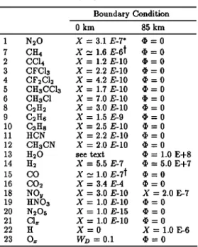
TABLE 2. Species or Family of Species for Which a Continuity Equation is Solved

Boundary Condition 0 km 85 km 1 N20 X = 3.1 E-7* ß = 0

7

CH4

X •_ 1.6 E-6• (• = 0

2 CC14 X = 1.2 E-10 ß = 0 3 CFCI• X = 2.2 E-10 (I) = 0 4 CF•CI• X = 4.2 E-10 (I) = 0 5 CH•CCI• X = 1.7 E-10 (I) = 0 6 CHIC1 X = 7.0 E-10 ß = 0 8 C•H• X = 3.0 E-10 (I) = 0 9 C•H• X = 1.5 E-9 (I) = 0 10 C•Hs X = 2.5 E-10 ß = 0 11 HCN X = 2.2 E-10 (I) = 0 12 CH•CN X = 2.0 E-10 (I) = 0 13 H20 see text (I) = 1.0 E+8 14 H2 X = 5.5 E-7 (I) = 5.0 E+7

15 CO X "- 1.0 E-7• (I) = 0

16 CO2 X = 3.4 E-4 (I) = 0

18 N Oy X = 3.0 E-10 X = 2.0 E-7

19 HNO• X = 1.0 E-10 (I) = 0 20 N•O5 X -- 1.0 E-15 (I) = 0 21 CI• X = 1.0 E-10 (I) = 0

22 H X=0 X=I.0E-6

23 O• Wz) = 0.1 (I) = 0

Adopted boundary conditions are given at the Earth

surface (0 km) and at the mesopause (85 km). X is mixing ratio; (I) is flux (cm -2 s-l). WD is deposition ve- locity (cm s -1. Species in photochemical equilibrium or

whose concentration is derived from a transported fam-

ily are 03, O(3P), O(1D), OH, HO2, CH302, N, NO2,

NO3, HObNOb, C1, C10, HOC1, HC1, and C1ONO•. * Read 3.1 E-7 as 3.1 x 10 -?.

lVariable with latitude.

this component would not improve the validity of the

results.

For the short-lived chemical species with a lifetime shorter than the dynamical time constants, photochemical equilibrium conditions apply and the concentration of

trace gas /is derived

from an algebraic

equation

S'• (Xi)

continuity is solved (and the boundary conditions

imposed

on these species)

as well as of those which are assumed

to

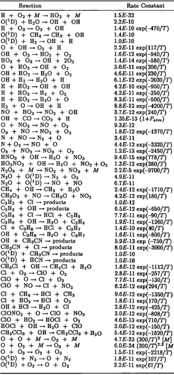
be in photochemical equilibrium. The different reactions

introduced in the model with the related reaction rates

based on the Jet Propulsion Laboratory (JPL) 1985

compilation [DeMote et al., 1985] are given in Tables 3a,

3b, and 3c. The absorption cross sections used for the calculation of the photodissociation coefficients are very similar to the values suggested in the JPL 1985 tables.

Values of the solar irradiance are from Brasseur and Simon

[1981].

In order to avoid mathematically stiff systems due to the large dispersion in the lifetime of the several species, some of the fast-reacting constituents are grouped into more stable families for which a full continuity equation

(20) is solved. In our model, the following families

have been

formed:

O, = Oa + O(3p) + O(•D), NO•

= N + NO + NO2 + 2N205 + NOa + HNOa + HO2NO2 + C1ONO2, and C1, = C1 + C10 + HC1

+ HOC1 + C1ONO2. It should be noted that HNOa

and N205 are also calculated independently from the

NOu family because of their weak coupling with the

other odd nitrogen species, particularly at high latitude and in winter. The water vapor is transported in the stratosphere, but in the troposphere the relative humidity

is prescribed

according

to Cess [1976] and the mixing ratio

of H20 is calculated as a function of the local temperature and pressure. The concentration of the individual fast- reacting species belonging to a given family are derived using relations based on the assumption of photochemical equilibrium.

3. MODEL RESULTS AND DISCUSSION

The model provides a large amount of output for differ- ent times of the year, and therefore only selected results

(primarily for solstice conditions)

will be presented

and

discussed. Additional results will be given in subsequent papers in which specific problems will be considered. 3.1. Radiation and Dynamics

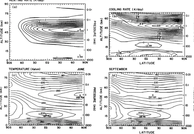
The deposition of energy in the stratosphere arises primarily from the absorption of solar radiation by the

Hartley band of ozone (200-300 nm). The heating rate

peaks near 50 km altitude with a maximum value (12.3

K/day) over the summer pole (see Figure 2a).

At

the equator, the 24 hour averaged heating rate reaches

a maximum value of about 10 K/day. The radiative

heating of the cloudless troposphere is due primarily to the radiative action of water vapor and the corresponding diabatic heating rate in this layer, where strong convective exchanges take place is only of the order of I K/day or less. At present, however, as was indicated earlier, tropospheric temperatures are specified from a climatology compiled by Randel [1987]. The contribution of molecular oxygen, which absorbs ultraviolet radiation at wavelengths shorter than 242 nm, remains smaller than about I

5644 BRASSEUR ET AL.: INTERACTIVE ,XIODEL OF THE MIDDLE ATMOSPHERE

TABLE 3a. Chemical Reactions Included in the Model and Corresponding Rate Constants

Reaction Rate Constant

H + O•+M--+HO• + M O(1D) +H•O•OH + OH H + 03-+02 + OH O(•D) + CH4-+CHs q- OH O(•D) + H•.-•OH + H 0 + OH-+O•. + H OH + O3--+ HO• + O• HO• + O3--+OH + 20• O + HO•--+OH + O• OH+HO•. •H20 + 0•. OH+H2-+H•.O + H H + HO2-+OH + OH H + HO2--+H2 + O• H + HO2-+H20 + O H•. + O-+OH + H NO + HO2-+ NO2 + OH OH + CO•CO•. + H O + NO2--+NO + O•_ O3 + NO--+ NO2 + O2 N + NO--+N2 + O N+O2-+NO + O 03 + NO2-+ NO3 q- 02 HNOs + OH-+H20 + NOs

1.5E-32 2.2E-10 1.4E-10 exp(-470/T) 1.4E-10 1.0E-10 2.2E-11 exp(117/T) 1.6E-12 exp(-940/T) 1.4E-14 exp(-580/T) 3.0E-11 exp(200/T) 4.6E-11 exp(230/T) 6.1E-12 exp(-2030/T) 4.2E-10 exp(-950/T) 4.2E-11 exp(-350/T) 8.3E-11 exp(-500/T) 8.8E-12 exp(-4200/T) 3.7E-12 exp(240/T) 1.35E-13 (I+P•,,•) 9.3E-12 1.8E-12 exp(-1370/T) 3.4E-11 4.4E-12 exp(-3320/T) 1.2E-13 exp(-2450/T) 9.4E-15 exp(778/T)

HO2NO2 + OH--, H20 + NO2 + 02 1.3E-12 exp(380/T)

N205 + M--+ NO2 + NOs + M 2.2E-5 exp(-9700/T)

N20 + O(1D)-+N•. + 0•.

N•.O + O(1D)•NO + NO

CH4 q- OH-+ CHs q- H20 CHsO2 + NO-+ CHsO + NO•. C2H2 + C1--+ products C2H2 + OH--+ products C2Ht; + C1 -+ HC1 + C2H5 C2H6 q- OH-+ H20 q- C2H5 CI q- C3H 8 --+ HC1 + Call7 OH q- C3H8 --+ H20 + C3H7 OH q- CHsCN --+ products CHsCN q- C1 --• products O(1D) + CHsCN--, products O(•D) + HCN --+ products CHsC1 + OH-+ CH2C1 + H20 C1 + 03--* ClO + O2 ClO + O-,C1 + O2

ClO + NO-+C1 + NO•.

C1 q- CH4-•HC1 q- CHs C1 + H02--* HC1 + 02 OH + He1 --+ H20 + C1 C1ONO2 q- O--+ C10 q- NOs ClO + HO2-,HOC1 + 02 HOCI q- OH-•H20 q- ClO

CHsCCls q- OH--, CH2CCls q-H20 0 + 0 + M•02 + M 0 + 02 + M•03 + M O + O3->O2 + 02 O(1D) + N2--+O + N2 O(1D) +02 •0 + 02 4.9E-11 6.7E-11 2.4E-12 exp(-1710/T) 4.2E-12 exp(180/T) 1.0E-12 6.5E-12 exp(-650/T) 7.7E-11 exp(-90/T) 1.9E-11 exp(-1260/T) 1.4E-10 exp(40/T) 1.6E-11 exp(-S00/T) 5.9E-13 exp (-750/T) 8.0E-11 exp(-3000/T) 1.0E-10 1.0E-10 1.8E-12 exp(-1112/T) 2.8E-11 exp(-257/T) 7.7E-11 exp(-130/T) 6.2E-12 exp(294/T) 9.6E-12 exp(-1350/T) 1.8E-11 exp(170/T) 2.8E-12 exp(-425/T) 3.0E-12 exp(-808/T) 4.6E-13 exp(710/T) 3.0E-12 exp(-150/T) 5.4E-12 exp(-1820/T)

4.7E-33

(300/T)_

2

the atmospheric

density

(cm-S),

Paur,

is the pressure

expressed

in

K/day below the mesopause, although this constituent is the largest contributor to solar heating in the upper

mesosphere. The cooling (Figure 2b) resulting from

the emission of infrared radiation by carbon dioxide, ozone, and water vapor is nearly in balance with the solar heating in the illuminated part of the atmosphere. In these regions the temperatures calculated by the model are similar to radiative equilibrium conditions. In the polar region during winter, when no solar light is

available, the cooling (of as much as 7 K/day at 60-

TABLE 3b. Three-Body Reaction With the Following Expressions

for Their Rate Constant k (cm 3 s -1)

Rate Exponent

NOs + NO2 + M -, N205 + M t• o .300 2.2 E-30 naooøø = 1.0 E-12 NO2 + OH + M -• HNOs + M .s00 = 2.6 E-30

•0 = 2.4 E-11 NO2 + HO2 + M -• HO2NO2 + M t% .300 = 2.3 E-31 o

•soo = 4.2 E-12

CIO + NO2 + M --• C1ONO2 + M naoøø = 1.8 E-31

•soo = 1.5 E-11 n=2.8 m=0 n=2.9 rn = 1.3 n=4.6 m=O n=3.4 m=1.9

The rate constant is derived by k = [t%[M]/(1 + t•o [M]/•oo)]

ß 300

0.6

{•+[•ø•ø(•ø[M]/•=)]•}-•

with •:o

= .3oo

(T/300)-" and

• = •

km altitude) is counterbalanced

by compressional

heating

through substantial downward motion of air. In the lower stratosphere, where the radiative time constant is larger than 10 days, the meridional circulation plays a dominant role in establishing the temperature distribution.

The meridional distribution of the temperature obtained by solving the thermodynamic equation, in which radia- tive transfer and heat transport are included explicitly, is shown in Figure 2c for June conditions. The stratopause maximum near 50-km altitude reaches a value of nearly 284 K over the summer pole but gradually decreases to- ward the winter pole. In the mesosphere the latitudinal gradient in the temperature is reversed as a consequence of momentum drag by gravity waves. The temperature at the mesopause is of the order of 170 K over the sum- mer pole and 220 K over the winter pole. With the adopted boundary conditions, a temperature minimum of about 205 K is derived at the tropopause over the tropics. There are differences between the two hemispheres for the

TABLE 3c. Photochemical Reactions Included in the Model Reaction s(o,) s'(o,) 7(o3) s'(oa) S(H,O) S(NO) S(CO,) S(CH4) S(NO) J(HNOs) J(CF2C12) J(CFC13) J(CC14) J(ItOCl) J(CH3CC13) J(HO2NO2) S(CHC0 S(C•ONO•) S(N•O•) S(NO) 02 q- hv --• o(sr) q- O(SP) 02 q- hv --+ O(1D) q- O(sP) Os + h•, --+ O(S_P) + 02 03+h•'•O(•D)+02 H20 + h•, --+ OH + H N20 + h•, --+ N2 + O(•D) CO2 +h•,•CO+O CH4 + h•, --+ products NO2 + hy --+ NO + O(3p) fiNOs + h• -• NO2 + OH CF2C12 q- h•, --, CF2CI q- C1 CFCIs + ht, -• CFC12 + C1 CC14 + h•, --+ CCls + C1 HOG1 + h•, --+ C10 + H CHsCCIs + h•, • CHsCC12 + C1 HO2NO2 + h•, -• NO2 + HO2 CHsC1 + hy -• CHs + C1 ClONO2 + h•, --+ NOs + C1 N205 + h•, --+ NO2 q- NOs NO + h•,--+ N + O

BRA$$gUR BT AL ß INTER. ACTIVE MODBL OF THB MIDDLE ATMOSPHERB 5645 9O 75 E 60 :::) 45 <• 30

HEATING RATE (K/day)

I I I I I J I I I I I J I I I I I J I I I I I J I I I I I J I I I I I a '--""-- I -•---.-.-.-...• _ _ _ - I o 9os -,tlilllliilllliillll•,,l,,•,,li,iil I000 60 30 EQ 30 60 90N

O.Ot COOLING RATE (K/day)

O.I

5

ß

.._.,

•0•---'-••

'"

. 1

'øø

o

....

ooo

eos eON

TEMPERATURE (Kelvin) JUNE

/ • • • •V I I/I I I/,q I • I I--I-...I.•k• III I I I r'-,• i i I i I/

• (c) • ••

•,•o•

• o.ol

/

_,oo

/,ooo

.• 60 •

30

ß

'o -• 60

o r-•

,, qs?,,,

•/iooo

Fig. 2. Meridional distribution of (a) the solar heating rate and (b) the infrared cooling rate expressed in Kelvins

per day (June

conditions),

and

meridional

distribution

of the zonally

averaged

temperature

(expressed

in Kelvins),

(c) in June

and (d) in September.

Contour

intervals:

1 K/day (Figure

2a), 0.7 K/day (Figure

2b),

and 10 K (Figures

2c and 2d).

same season, those being direct consequences of the lati- tudinal asymmetry in the specified dynamical conditions at the 15-km boundary. For example, the temperature in

the lower stratosphere

(20 km) is of the order of 185-

190 K over Antarctica in September (Figure 2d) but is

nearly 10 K warmer over the Arctic 6 months later. This difference between the two hemispheres is consistent with climatologicM data and explains the more frequent pres- ence and the different nature of polar stratospheric clouds

in winter over Antarctica than over the Arctic.

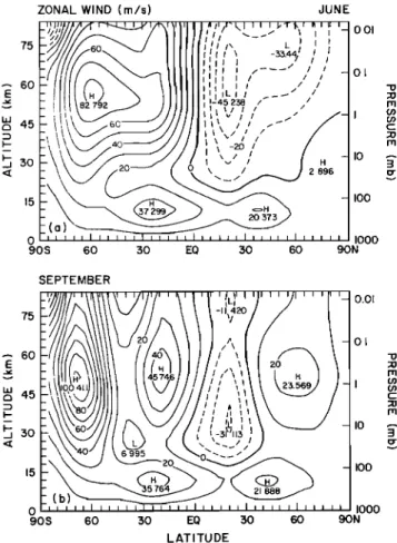
The zonal wind, in gradient balance with the tempera- ture, is shown for June and September in Figures 3a and 3b. For solstice conditions, the westerly wind in the south-

ern hemisphere

(winter) reaches

a velocity of 90 m/s near

the stratopause

at 60

ø. In the northern

hemisphere

(sum-

mer) the easterly winds are a factor of 2 weaker (about

40 m/s in the upper stratosphere

and in the mesosphere).

In September the model produces a strong polar vortex in the southern hemisphere with a maximum wind velocity

of 100 m/s near the stratopause between 600 and 700 lat-

itude. A substantially weaker stratospheric jet is found 6

months later in the springtime

northern hemisphere

(not

shown)

with maximum wind speed

of 88 m/s.

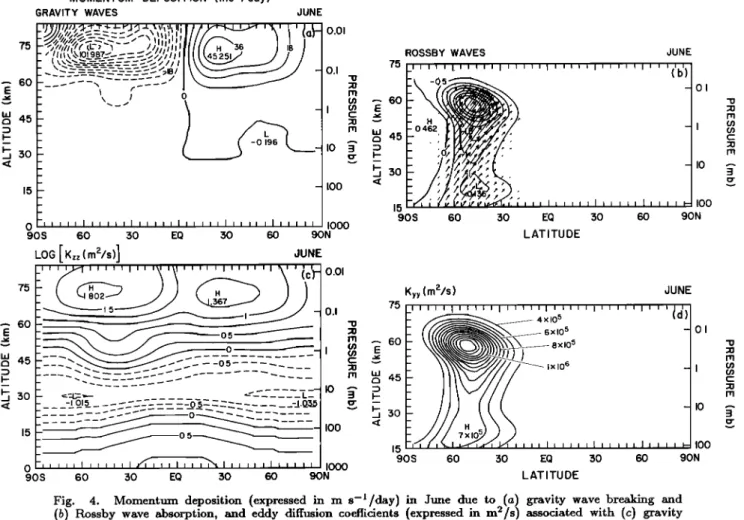
The momentum sources from gravity and Rossby wave

absorption are shown in Figures 4a and 4b, respectively.

A large easterly

torque

of more than 100 m s-i/day is

derived in the winter mesosphere, while a westerly drag

of up to 50 m s -z/day is calculated

in the summer

meso-

Eliassen-Palm

flux, which is shown by the arrows in Fig-

ure 4b, is directed upward and toward the equator. The torque associated with Rossby wave absorption is for this

particular

case

in the range 0.5 to 6 m s-l/day in the

latitudinal band of 300 to 600 . The eddy diffusion coef-

ficients used in the transport scheme of the model and

derived from the parameterization

of wave breaking are

shown for June conditions in Figures 4c and 4d. The

vertical eddy diffusivity, as derived from the gravity wave

formulation,

is characterized

by a strong vertical gradient

in the stratosphere. Kzz coefficients of the order of 1 to

70 m2/s are calculated

above

the stratopause,

with the

highest values above the westerly jet core. In the lower stratosphere, below the breaking level of the waves, small

background

values

of the order of 0.1 m2/s are adopted.

In the troposphere, where rapid vertical mixing occurs,

values

of the order of 5-10 m2/s are specified

with a

variation in latitude to account for the varying height of the tropopause. The meridional diffusivity associated with planetary wave absorption for the particular case shown

in Figure 4d reaches values of the order of (0.5-2.0) x

106 m2/s at mid-latitude.

In the summer

hemisphere,

5646 BRASSEUR ET AL.: INTERACTIVE MODEL OF THE MIDDLE ATMOSPHERE

ZONAL WIND m/s) JUNE

._

h'/•i,?ll//r

•

7•' ¾1'1' •__ , , - o.o,

I000

90 S 60 50 EO 50 60 90N SEPTEMBER

' i" p,' , ';' "Y" ' "

oo,

/• 0.1

0

90S 60 50 EO 50 60 90N

LATITUDE

Fig. 3. Meridional distribution of the zonal wind (expressed in

meters per second), (a) in June and (b) in September. Contour

intervals: 10 m/s.

where no planetary waves

penetrate,

a background

value

of 3 x 10

5 m2/s is adopted

to account

for subgrid

mixing

processes.

Finally, the transformed

mean Eulerian meridional

cir-

culation,

driven by momentum

drag associated

with grav-

ity and planetary

wave dissipation,

is shown

in Figures

5a

cells affecting

the temperature

and the density of trace

gases

in both hemispheres

are clearly

visible.

Because

the

boundary conditions

on the stream function specified

at

15 km are not symmetric on each side of the equator, the flow in the northern hemisphere tends to transport

mass and energy all the way to the pole in the northern

hemisphere

while it reaches

only a region

near 600-700

sequence

of this hemispheric

difference

is that the model

diagnoses

the Antarctic region to be closer to radiative

equilibrium conditions

in winter than the Arctic during

the same season. Because polar night temperatures over Antarctica are relatively cold, radiative cooling in this

region is small. The net heating becomes

transitorily pos-

itive and reaches

about 0.3 K/day near 30-km altitude, as

the Sun returns over Antarctica in late winter. Since the

vertical velocity specified at 15 km as boundary condition

is zero over the region of the South Pole (see Figure 1),

the model therefore predicts some upwelling during this short transition period but its strength, which is not large

enough to deplete ozone significantly,

is highly dependent

on the ozone density in the lower polar stratosphere. This

upward flow will be substantially reduced and even sup-

pressed if ozone gets destroyed by chemical processes in

late winter or early spring, as has been observed since the

late 1970s (Furman et al. [1985] and others; see Solomon.

[•988] or Brasseur

et al., [1988a1

for a review). A more

refined analysis of the dynamical conditions in the polar re•ions in winter and sprin• requires a three-dimension• study describin• exchanges between the troposphere and the stratosphere and accountin• for the full interactions between chemistry, radiation, and dynamics. The present twodimensional model, however, is capable of describing the net meridional transport in some det•l and accounts for hemispheric differences in the tropospheric forcing of stratospheric dynamics.

3.œ. Chemistry

The distribution of selected trace constituents will now

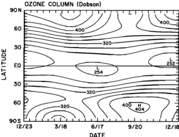
be presented with the purpose of validating the model formulation. Figures 6a and 6b present the calculated

distributions of nitrous oxide and methane for June con-

ditions. In both cases the Hadley cell, through which these gases are transported from the troposphere into the stratosphere, produces the high mixing ratios over the tropics in the stratosphere. The meridionM slope of the isomixing ratio contours between 15- and 40-km altitude results from the opposing action of the meridionM circu-

lation (which tends to enhance the latitudinal gradients)

and eddy diffusion (which tends to mix the trace gases

along the quasi-horizontal

isentropes) [see Holton, 1981].

SeasohM variations in the mixing ratio, driven by the Sun, can be seen in the upper stratosphere and meso- sphere, where the photochemical time constant is smaller than the characteristic timescale for transport. Hence the effect of the chemistry is most pronounced in the summer hemisphere and is stronger for N20 than for CH4 as a re- sult of the photochemical lifetime's being 10 times larger for CH4 than for N20 at 60 km and 60øN in June. The decrease with Mtitude of the mixing ratio in the meso- sphere is reduced by vertical mixing resulting from gravity wave breaking. Since in our model, vertical eddy diffusiv- ity is strongest near the core of the stratospheric jets and is substantially weaker in the tropics, a weak double peak

structure appears occasionally in the meridional distribu-

tion of the source gases. Such a structure, to be compa-

rable to the global observations

of the stratospheric

and

mesospheric

sounder

(SAMS) instrument

[Jones

and Pyle,

1984], requires the presence

of an additional momentum

source located in the tropics. Gray and Pyle [1986] have

attributed such a source to the absorption in the strato- sphere of Kelvin waves. Finally, the distribution of the

source gases in the mesosphere depends on the strength

of the meridional circulation, which is directed from the summer to the winter hemisphere. The strength of this cell is determined by the momentum deposition of gravity waves in the mesosphere and upper stratosphere.

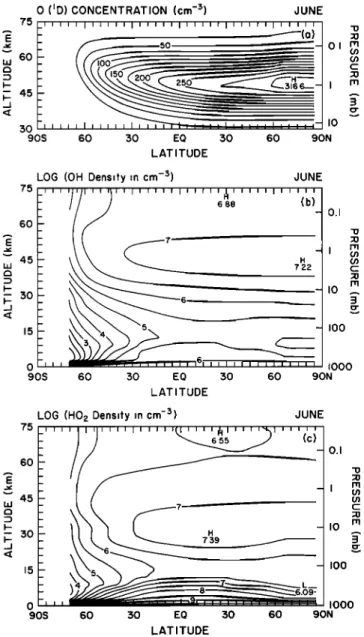
The distribution of water vapor in the middle atmo- sphere is shown in Figure 7a. In the lower stratosphere, where H20 is a purely conservative tracer, the slope of the mixing ratio lines is determined by the strength of the meridional flow. Clearly, the model underpredicts the mixing ratio of water vapor at high latitudes. A rea- son for the discrepancy between calculated and observed distributions could be an improper representation of trans-

75 --- 6O E • 4,5 _j $0 75 --- 6O E _j $0 o 9os o 9os 60 30 EQ 30 60 90N

LOG

[Kzz

(mZ/s)]

JUNE

' ' ' '

' ' ' ' ' I ' ' ' ' • I ' ' '' ' I ' ' • ' ' I ' ' iCW

-o.,

_- -

- - ...

- ....

I •---L---

•

'-•--•

L

--

IO

Ii,-,-,

_

_

_

MOMENTUM DEPOSITION (ms-•/doy)

GRAVITY WAVES JUNE

"._•,.•J..I".,J•-L•,\I'•II,|I•IIJJ I,/-"1'""'!•_1 I • I•L I I I / I/

:

o.o,

I

Ioo

<

'

'

ROSSBY WAVES JUNE

75 _•

• • [ • i • • • • • I • t t [ • I t • • • • I • • • • • I • • •(•b

•)

Kyy

(mZ/s)

JUNE

_ Illlllll]111111111

_••

_4x,o

₅

IIIIIIIII

III I Ill

_d:

x IO 6 I

60 :30 EQ :30 60 90N

LATITUDE

Fig. 4. Momentum

deposition

(expressed

in m s -l/day) in June due to (a) gravity wave breaking

and

(b) Rossby

wave

absorption,

and eddy diffusion

coefficients

(expressed

in m2/s) associated

with (c) gravity

wave breaking and (d) Rossby wave absorption. The vectors in Figure 4b are proportional to the Eliassen-

Palm flux (maximum

vector length, 2.7 x 108 kg m -1 s-2). Note in the case of Figure 4c that the

diffusivity is represented by its decimal logarithm and that the specified tropospheric values are also represented.

Contou•

intervals:

9 m s -•/day (Figure

4a), 0.5 m s -•/day (Figure

4b), 0.25 (Figure

4c), and 1 x 105 m2/s

(Figure 4d). 0.1 100 0.1 100 "13 :;13 C:: :;13

MERIDIONAL CIRCULATION JUNE LOG (N20 M,xing Rat,o) JUNE

75 /I I I I I I I I I I I/ I I I\1 ',1 •d,-'l--I--.I-..l_.] r'-I i',,I

I- .-_ ... _a•... x •.. • • x• •xx,•xxx x "--I U.UI 0.1 I- --- • • • " "r•r• '" -104 x x •. • •. i

.... F ..-

..--•,-...-.:--__--.:..-..-...;-1o.• •

15

I00

15

I00

LOG (CH 4 Mixtng Ratio) JUNE

I_l

I I I I r,.11

i---i-.i

i r--I..l•l•l•E•-I-_t:l--_l_-_[--_l:l_-•_l-q•l•l•l•fi

..-..

75

...

,-_._t-:----•:=t:.:t--:t:--_/

45 - /

/ / / "'"

- -- '""'"

'• • '•'"

'"

• -½479 m

<•

:_-%S;..-;.--_

....

so_---"-L--"j•-•

a

:30_

IO •

15 -I--I-I;-•--I'•"['•

• • I I I •1•

•1 •tt •F-Im-•-•-•--r-

I00

9()S 60 :30 EQ :30 60 90N

LATITUDE

Fig. 6. Meridional distribution (June conditions) of the zonally

averaged mixing ratio of (a) nitrous oxide and (b) methane.

Contour intervals: 0.2.

90S 60 30 EQ 30 60 90N LATITUDE

Fig. 5. Stream function of the transformed Eulerian mean merid-

ional circulation in (a) June and (b) September.

o 90 s 60 30 EQ 30 60 90N SEPTEMBER

E(b)• ...

•

•.lo,

o L,L

!/IL

,ooo