HAL Id: hal-01516246
https://hal.sorbonne-universite.fr/hal-01516246
Preprint submitted on 29 Apr 2017HAL is a multi-disciplinary open access
archive for the deposit and dissemination of sci-entific research documents, whether they are pub-lished or not. The documents may come from teaching and research institutions in France or abroad, or from public or private research centers.
L’archive ouverte pluridisciplinaire HAL, est destinée au dépôt et à la diffusion de documents scientifiques de niveau recherche, publiés ou non, émanant des établissements d’enseignement et de recherche français ou étrangers, des laboratoires publics ou privés.
A new result, for the box dimension of the graph of the
Weierstrass function
Claire David
To cite this version:
Claire David. A new result, for the box dimension of the graph of the Weierstrass function. 2017. �hal-01516246�
A new result, for the box dimension of the graph of the
Weierstrass function
Claire David
April 29, 2017Sorbonne Universités, UPMC Univ Paris 06
CNRS, UMR 7598, Laboratoire Jacques-Louis Lions, 4, place Jussieu 75005, Paris, France
1
Introduction
The determination of the box and Hausdorff dimension of the graph of the Weierstrass function has, since long been, a topic of interest. Let us recall that, given λ ∈ ]0, 1[, and b such that λ b > 1 + 3 π
2 , the Weierstrass function
x ∈ R 7→
+∞
∑
n=0
λncos (π bnx)
is continuous everywhere, while nowhere differentiable. The original proof, by K. Weierstrass [Wei72], can also be found in [Tit77]. It has been completed by the one, now a classical one, in the case where λ b > 1, by G. Hardy [Har11].
After the works of A. S. Besicovitch and H. D. Ursell [BU37], it is Benoît Mandelbrot [Man77] who particularly highlighted the fractal properties of the graph of the Weierstrass function. He also conjectured that the Hausdorff dimension of the graph is DW = 2 +ln λ
ln b. Interesting discussions in relation to this question have been given in the book of K. Falconer [Fal85]. A series of results for the box dimension can be found in the works of J.-L. Kaplan et al. [KMPY84], where the authors show that it is equal to the Lyapunov dimension of the equivalent attracting torus, and in those by T-Y. Hu and K-S. Lau [HL93]. As for the Hausdorff dimension, a proof was given by B. Hunt [Hun98] in 1998 in the case where arbitrary phases are included in each cosinusoidal term of the summation. Recently, K. Barańsky, B. Bárány and J. Romanowska [BBR17] proved that, for any value of the real number b, there exists a threshold value λb belonging to the interval
] 1
b, 1
[
such that the aforemen-tioned dimension is equal to DW for every b in ]λb, 1[. Results by W. Shen [She15] go further than the
ones of [BBR17]. In [Kel17], G. Keller proposes what appears as a much simpler and very original proof. In our work [Dav17], where we build a Laplacian on the graph of the Weierstrass function, we came across a simpler means of computing the box dimension of the graph, using a sequence a graphs that approximate the studied one. Results are exposed in the sequel.
2
Framework of the study
In this section, we recall results that are developed in [Dav17].
Notation. In the following, λ and Nb are two real numbers such that:
0 < λ < 1 , Nb ∈ N and λ Nb > 1
We will consider the (1−periodic) Weierstrass function W, defined, for any real number x, by:
W(x) =
+∞
∑
n=0
λn cos (2 π Nbnx)
We place ourselves, in the sequel, in the Euclidean plane of dimension 2, referred to a direct or-thonormal frame. The usual Cartesian coordinates are (x, y).
The restriction ΓW to [0, 1[×R, of the graph of the Weierstrass function, is approximated by means of a sequence of graphs, built through an iterative process. To this purpose, we introduce the iterated function system of the family of C∞ contractions fromR2 toR2:
{T0, ..., TNb−1}
where, for any integer i belonging to{0, ..., Nb− 1}, and any (x, y) of R2:
Ti(x, y) = ( x + i Nb , λ y + cos ( 2 π ( x + i Nb ))) Property 2.1. ΓW = N∪b−1 i=0 Ti(ΓW)
Definition 2.1. For any integer i belonging to{0, ..., Nb− 1}, let us denote by:
Pi= (xi, yi) = ( i Nb− 1 , 1 1− λ cos ( 2 π i Nb− 1 ))
the fixed point of the contraction Ti.
We will denote by V0 the ordered set (according to increasing abscissa), of the points:
{P0, ..., PNb−1}
The set of points V0, where, for any i of{0, ..., Nb− 2}, the point Pi is linked to the point Pi+1,
con-stitutes an oriented graph (according to increasing abscissa)), that we will denote by ΓW0. V0 is called the set of vertices of the graph ΓW0.
For any natural integer m, we set:
Vm= N∪b−1
i=0
Ti(Vm−1)
The set of points Vm, where two consecutive points are linked, is an oriented graph (according to
increasing abscissa), which we will denote by ΓWm. Vm is called the set of vertices of the graph ΓWm.
We will denote, in the sequel, by
NS
m = 2 Nbm+ Nb− 2
the number of vertices of the graph ΓWm, and we will write: Vm=
{
Sm
0 ,S1m, . . . ,SNmm−1
}
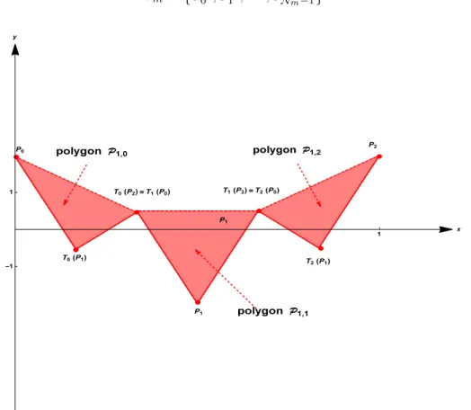
Figure 1: The polygonsP1,0,P1,1,P1,2, in the case where λ =
1
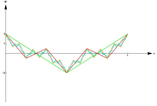
Figure 2: The graphs ΓW0 (in green), ΓW1 (in red), ΓW2 (in orange), ΓW (in cyan), in the case where λ = 1
2, and Nb= 3.
Definition 2.2. Consecutive vertices on the graph ΓW
Two points X et Y de ΓW will be called consecutive vertices of the graph ΓW if there exists a natural integer m, and an integer j of{0, ..., Nb− 2}, such that:
X = (Ti1◦ . . . ◦ Tim) (Pj) et Y = (Ti1 ◦ . . . ◦ Tim) (Pj+1) {i1, . . . , im} ∈ {0, ..., Nb− 1}
m
or:
X = (Ti1 ◦ Ti2 ◦ . . . ◦ Tim) (PNb−1) et Y = (Ti1+1◦ Ti2. . .◦ Tim) (P0)
Definition 2.3. For any natural integer m, the NmS consecutive vertices of the graph ΓWm are, also,
the vertices of Nbm simple polygons Pm,j, 06 j 6 Nbm− 1, with Nb sides. For any integer j such
that 06 j 6 Nbm− 1, one obtains each polygon by linking the point number j to the point num-ber j + 1 if j = i mod Nb, 06 i 6 Nb− 2, and the point number j to the point number j − Nb+ 1
if j =−1 mod Nb. These polygons generate a Borel set ofR2.
Definition 2.4. Word, on the graph ΓW
Let m be a strictly positive integer. We will call number-letter any integer Mi of {0, . . . , Nb− 1},
and word of length |M| = m, on the graph ΓW, any set of number-letters of the form:
M = (M1, . . . ,Mm)
We will write:
Definition 2.5. Edge relation, on the graph ΓW
Given a natural integer m, two points X and Y of ΓWm will be calledadjacent if and only if X and Y
are two consecutive vertices of ΓWm. We will write: X ∼
m Y
This edge relation ensures the existence of a word M = (M1, . . . ,Mm) of length m, such that X
and Y both belong to the iterate:
TMV0 = (TM1 ◦ . . . ◦ TMm) V0
Given two points X and Y of the graph ΓW, we will say that X and Y are adjacent if and only if there exists a natural integer m such that:
X ∼
m Y
Proposition 2.2. Adresses, on the graph of the Weierstrass function
Given a strictly positive integer m, and a word M = (M1, . . . ,Mm) of length m ∈ N⋆, on the
graph ΓWm, for any integer j of{1, ..., Nb− 2}, any X = TM(Pj) de Vm\ V0, i.e. distinct from one of the Nb fixed point Pi, 06 i 6 Nb− 1, has exactly two adjacent vertices, given by:
TM(Pj+1) et TM(Pj−1)
where:
TM = TM1◦ . . . ◦ TMm
By convention, the adjacent vertices of TM(P0) are TM(P1) and TM(PNb−1), those of TM(PNb−1), TM(PNb−2) and TM(P0) .
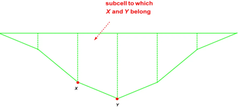
Definition 2.6. mth−order subcell, m ∈ N⋆, related to a pair of points of the graph ΓW Given a strictly positive integer m, and two points X and Y of Vm such that X∼
mY , we will call
mth−order subcell, related to the pair of points (X, Y ), the polygon, the vertices of which
are X, Y , and the intersection points of the edge between the vertices at the extremities of the polygon, i.e. the respective intersection points of polygons of the type Pm,j−1 and Pm,j, 16 j 6 Nbm− 1, on
the one hand, and of the type Pm,j andPm,j+1, 06 j 6 Nbm− 2, on the other hand.
Notation. For any integer j belonging to{0, ..., Nb− 1}, any natural integer m, and any word M of
length m, we set: TM(Pj) = (x (TM(Pj)) , y (TM(Pj))) , TM(Pj+1) = (x (TM(Pj+1)) , y (TM(Pj+1))) Lm = x (TM(Pj+1))− x (TM(Pj)) = 1 (Nb− 1) Nbm , hj,m = y (TM(Pj+1))− y (TM(Pj))
Figure 3: A mth−order subcell, in the case where λ = 1
2, and Nb= 7.
Proposition 2.3. An upper bound and lower bound, for the box-dimension of the graph ΓW For any integer j belonging to{0, 1, . . . , Nb− 2}, each natural integer m, and each word M of length m,
let us consider the rectangle, the width of which is:
Lm = x (TM(Pj+1))− x (TM(Pj)) =
1 (Nb− 1) Nbm
and height |hj,m|, such that the points TM(Pj+1) and TM(Pj+1) are two vertices of this rectangle.
Then: L2−DW m (Nb− 1)2−DW {1− λ2 min 06j6Nb−1 sin ( π (2 j + 1) Nb− 1 ) − π Nb(Nb− 1) (λ Nb− 1) } 6 |hj,m| and: |hj,m| 6 η2−DWL2m−DW
where the real constant η2−DW is given by :
η2−DW = 2 π2(Nb− 1)2−DW { (2 Nb− 1) λ (Nb2− 1) (Nb− 1)2(1− λ) (λ Nb2− 1) + 2 Nb (λ Nb2− 1) (λ Nb3− 1) }
There exists thus a positive constant C = max { (Nb− 1)2−DW { 2 1− λ 06j6Nminb−1 sin ( π (2 j + 1) Nb− 1 ) − π Nb(Nb− 1) (λ Nb− 1) } ,η2−DW }
such that the graph ΓW on Lm can be covered by at least and at most:
Nm { C ( Lm Nm )1−DW + 1 } = C L1−DW m NmDW + Nm
squares, the side length of which is Lm Nm
.
Proof. For any pair of integers (im, j) of{0, ..., Nb− 2}2:
Tim(Pj) = ( xj+ im Nb , λ yj+ cos ( 2 π ( xj+ im Nb )))
For any pair of integers (im, im−1, j) of {0, ..., Nb− 2}3:
Tim−1(Tim(Pj)) = (xj+im Nb + im−1 Nb , λ2yj+ λ cos ( 2 π ( xj + im Nb )) + cos ( 2 π (xj+im Nb + im−1 Nb ))) = ( xj + im Nb2 + im−1 Nb , λ2yj+ λ cos ( 2 π ( xj + im Nb )) + cos ( 2 π ( xj+ im Nb2 + im−1 Nb )))
For any pair of integers (im, im−1, im−2, j) of{0, ..., Nb− 2}4:
Tim−2 ( Tim−1(Tim(Pj)) ) = ( xj+ im Nb3 + im−1 Nb2 + im−2 Nb , λ3yj+ λ2 cos ( 2 π (x j+im Nb )) +λ cos ( 2 π ( xj+ im Nb2 + im−1 Nb )) + cos ( 2 π ( xj+ im Nb3 + im−1 Nb2 + im−2 Nb )) )
Given a strictly positive integer m, and two points X and Y of Vm such that:
X ∼
m Y
there exists a wordM of length |M| = m, on the graph ΓW, and an integer j of{0, ..., Nb− 2}2, such
that:
X = TM(Pj) , Y = TM(Pj+1)
Let us write TM under the form:
TM= Tim◦ Tim−1◦ . . . ◦ Ti1 where (i1, . . . , im) ∈ {0, ..., Nb− 1}m.
One has then:
x (TM(Pj)) = xj Nbm + m ∑ k=1 ik Nbk , x (TM(Pj+1)) = xj+1 Nbm + m ∑ k=1 ik Nbk
and: y (TM(Pj)) = λmyj+ m ∑ k=1 λm−kcos ( 2 π ( xj Nk b + k ∑ ℓ=0 im−ℓ Nbk−ℓ )) y (TM(Pj+1)) = λmyj+1+ m ∑ k=1 λm−kcos ( 2 π ( xj+1 Nk b + k ∑ ℓ=0 im−ℓ Nbk−ℓ ))
This leads to:
hj,m− λm (yj+1− yj) = m ∑ k=1 λm−k { cos ( 2 π ( xj+1 Nbk + k ∑ ℓ=0 im−ℓ Nbk−ℓ )) − cos ( 2 π ( xj Nbk − k ∑ ℓ=0 im−ℓ Nbk−ℓ ))} = −2 m ∑ k=1 λm−k sin ( π ( xj+1− xj Nbk )) sin ( 2 π ( xj+1+ xj 2 Nbk + k ∑ ℓ=0 im−ℓ Nbk−ℓ ))
Taking into account:
λm (yj+1− yj) = λm 1− λ ( cos ( 2 π (j + 1) Nb− 1 ) − cos ( 2 π j Nb− 1 )) = −2 λ m 1− λ sin ( π Nb− 1 ) sin ( π (2 j + 1) Nb− 1 ) one has: hj,m+ 2 λm 1− λ sin ( π Nb− 1 ) sin ( π (2 j + 1) Nb− 1 ) = −2 m ∑ k=1 λm−ksin ( π Nbk+1(Nb− 1) ) sin ( π (2 j + 1) Nbk+1(Nb− 1) + 2 π k ∑ ℓ=0 im−ℓ Nbk−ℓ ) Thus: y (TM(Pj))− y (TM(Pj+1))− 2 λm 1− λ sin ( π Nb− 1 ) sin ( π (2 j + 1) Nb− 1 ) 6 ∑m k=1 2 π λm−k Nbk+1(Nb− 1) = π λm (1− 1 λmNm b ) λ NbNb(Nb− 1) ( 1−λ N1 b ) 6 π λm Nb(Nb− 1) (λ Nb− 1)
which leads to:
y (TM(Pj))− y (TM(Pj+1)) > 2 λm 1− λ sin ( π Nb− 1 ) sin ( π (2 j + 1) Nb− 1 ) − π λm Nb(Nb− 1) (λ Nb− 1) or:
y (TM(Pj+1))− y (TM(Pj)) > 2 λm 1− λ sin ( π Nb− 1 ) sin ( π (2 j + 1) Nb− 1 ) − π λm Nb(Nb− 1) (λ Nb− 1)
Due to the symmetric roles played by TM(Pj) and TM(Pj+1), one may only consider the case when:
y (TM(Pj))− y (TM(Pj+1)) > 2 λm 1− λ sin ( π Nb− 1 ) sin ( π (2 j + 1) Nb− 1 ) − π λm Nb(Nb− 1) (λ Nb− 1) > 0 > λm { 2 1− λ 06j6Nminb−1 sin ( π (2 j + 1) Nb− 1 ) − π Nb(Nb− 1) (λ Nb− 1) }
The predominant term is thus:
λm= em (DW−2) ln Nb = Nm (DW−2)
b = L 2−DW
m (Nb− 1)2−DW
One also has:
|hj,m| 6 2 λm 1− λ π2(2 j + 1) (Nb− 1)2 + 2 m ∑ k=1 λm−kπ { 2 j + 1 (Nb− 1) Nbk + 2 k ∑ ℓ=0 im−ℓ Nbk−ℓ } π (Nb− 1) Nbk = 2 λ m 1− λ π2(2 j + 1) (Nb− 1)2 +2 π 2λm Nb− 1 m ∑ k=1 { (2 j + 1) λ−k (Nb− 1) Nb2k + 2 k ∑ ℓ=0 im−ℓλ−k Nb2k−ℓ } = 2 λ m 1− λ π2(2 j + 1) (Nb− 1)2 +2 π 2λm Nb− 1 { λ−1Nb−2(2 j + 1) (Nb− 1) (1− λ−mNb−2m) 1− λ−1Nb−2 + 2 m ∑ k=1 (Nb− 1) λ−k Nb2k 1− Nb−k−1 1− Nb−1 } 6 2 λm 1− λ π2(2 Nb− 1) (Nb− 1)2 +2 π 2λm Nb− 1 (2 Nb− 1) (Nb− 1) (1− λ−mNb−2m) λ N2 b − 1 +2 π 2λm Nb− 1 2λ −1N−2 b (Nb− 1) (1 − λ−mNb−2m) (1− Nb−1) (1− λ−1Nb−2) −2 π2λm Nb− 1 2λ −1N−3 b (Nb− 1) (1 − λ−mNb−3m) (1− Nb−1) (1− λ−1Nb−3) 6 2 λm 1− λ π2(2 Nb− 1) (Nb− 1)2 +2 π 2λm Nb− 1 (2 Nb− 1) (Nb− 1) 1 λ N2 b − 1 +4 π 2N bλm Nb− 1 { 1 λ N2 b − 1 − 1 λ N3 b − 1 } = 2 π2λm { (2 Nb− 1) λ (Nb2− 1) (Nb− 1)2(1− λ) (λ Nb2− 1) + 2 Nb (λ Nb2− 1) (λ Nb3− 1) }
Since: x (TM(Pj+1))− x (TM(Pj)) = 1 (Nb− 1) Nbm and: DW = 2 + ln λ ln Nb , λ = e(DW−2) ln Nb = N(DW−2) b
one has thus:
|hj,m| 6 2 π2L2m−DW (Nb− 1)2−DW { (2 Nb− 1) λ (Nb2− 1) (Nb− 1)2(1− λ) (λ Nb2− 1) + 2 Nb (λ N2 b − 1) (λ Nb3− 1) }
References
[BBR17] K. Barańsky, B. Bárány, and J. Romanowska. On the dimension of the graph of the classical Weierstrass function. Advances in Math., 2017.
[BU37] A. S. Besicovitch and H. D. Ursell. Sets of fractional dimensions. Notices of the AMS, 1937.
[Dav17] Claire David. Laplacian, on the graph of the Weierstrass function, arxiv:1703.03371, 2017. [Fal85] K. Falconer. The Geometry of Fractal Sets. Cambridge University Press, 1985.
[Har11] G. Hardy. Theorems connected with Maclaurin’s test for the convergence of series. The
Proceedings of the Royal Society of London, 1911.
[HL93] T.-Y. Hu and K.-S. Lau. Fractal dimensions and singularities of the weierstrass type functions. Transactions of the American Mathematical Society, 1993.
[Hun98] B. Hunt. The Hausdorff dimension of graphs of Weierstrass functions. Proc. Amer. Math.
Soc., 1998.
[Kel17] G. Keller. A simpler proof for the dimension of the graph of the classical Weierstrass function. Ann. Inst. Poincaré, 2017.
[KMPY84] J. Kaplan, J. Mallet-Paret, and J. Yorke. The Lyapunov dimension of a nowhere differen-tiable attracting torus. Ergodic Theory Dynam. Systems, 1984.
[Man77] B. B. Mandelbrot. Fractals: form, chance, and dimension. San Francisco: Freeman, 1977. [She15] Weixiao Shen. Hausdorff dimension of the graphs of the classical Weierstrass functions,
arxiv:1505.03986, 2015.
[Tit77] E. C. Titschmarsh. The theory of functions, Second edition. Oxford University Press, 1977. [Wei72] K. Weierstrass. Über continuirliche funktionen eines reellen arguments, die für keinen werth des letzteren einen bestimmten differentialquotienten besitzen, in karl weiertrass mathematische werke, abhandlungen ii. Akademie der Wissenchaften am 18 Juli 1872, 1872.