HAL Id: cea-01810693
https://hal-cea.archives-ouvertes.fr/cea-01810693
Submitted on 8 Jun 2018
HAL is a multi-disciplinary open access
archive for the deposit and dissemination of
sci-entific research documents, whether they are
pub-lished or not. The documents may come from
teaching and research institutions in France or
abroad, or from public or private research centers.
L’archive ouverte pluridisciplinaire HAL, est
destinée au dépôt et à la diffusion de documents
scientifiques de niveau recherche, publiés ou non,
émanant des établissements d’enseignement et de
recherche français ou étrangers, des laboratoires
publics ou privés.
Symbolic execution of transition systems with function
summaries
Imen Boudhiba, Christophe Gaston, Pascale Le Gall, Virgile Prévosto
To cite this version:
Imen Boudhiba, Christophe Gaston, Pascale Le Gall, Virgile Prévosto. Symbolic execution of
tran-sition systems with function summaries. 11th International Conference on Tests & Proofs, Jul 2017,
Marburg, Germany. �cea-01810693�
function summaries
?Imen Boudhiba1, Christophe Gaston2, Pascale Le Gall1 and Virgile Prevosto2
1 Laboratoire MICS, Grande Voie des Vignes, 92195 Chˆatenay-Malabry, France
email: {imen.boudhiba,pascal.legall}@centralesupelec.fr
2 CEA LIST, Point Courrier 174, 91191, Gif-sur-Yvette, France
email: {christophe.gaston,virgile.prevosto}@cea.fr
Abstract. Reactive systems can be modeled with various kinds of au-tomata, such as Input Output Symbolic Transition Systems (IOSTS). Symbolic execution (SE) applied to IOSTS allows computing constraints associated to IOSTS path executions (path conditions). In this context, generating test cases amounts to finding numerical input values satisfying such constraints using solvers. This paper explores the case where IOSTS models contain functions which are outside of the scope of such solvers. We propose to use function summaries which are logical formulas built from concrete values describing some representative input/output data tuples of the function. We define algorithmic strategies to solve path conditions including such functions based on techniques using and en-riching function summaries. Our method has been implemented within the Diversity tool and has been applied to several examples.
Keywords: Input Output Symbolic Transition Systems, Functions sum-maries, Symbolic Execution, Transition coverage.
1
Introduction
Many testing theories and algorithms use Symbolic Execution (SE) techniques [10]. In the last decade, it has received much attention and has been incorporated in several testing tools such as NASA’s Symbolic (Java) PathFinder [29], UIUC’s CUTE and jCUTE [21], UC Berkeley’s CREST [13], and the CEA’s PathCrawler [28] and DIVERSITY tools [15]. In particular, for the latter one, SE has been adapted for models using variants of abstract labeled transition systems, namely Input Output Symbolic Transition Systems (IOSTS) [17]. Symbolic trees representing all possible execution paths of the model (up to some coverage goals) are com-puted by executing the model with variables instead of concrete values. For a particular path, a constraint on these variables, called path condition, charac-terizes concrete values ensuring its execution. Sequences of concrete test inputs
?Part of this work has been conducted within the French PIA project SESAM Grids
2012-2016 [12] and the Vessedia project funded from European Union’s Horizon 2020 research and innovation programme under grant agreement No 731453.
exercising a given path are computed by solving the corresponding path con-dition. As is the case for programs, one of the main limits of this approach is that the usage of some particular functions in the model may make the process inapplicable, either because their symbolic analysis would cause combinatorial explosion in the number of paths to be considered, or because they contain op-erations that go beyond the capacity of the solver used, or even simply because they are black box functions from the model point of view. This latter situation occurs for example when the modeler makes a reference to an executable function without accessible source code in its model (or without source code processable by the SE tool). In this paper, we call such functions external functions and they are assumed to be functionally correct (i.e. we suppose that we have a reference implementation for each of the external functions used in the model). In the frame of Model-based Testing [33], a classical way to deal with this situation is to fully abstract external functions by considering the results of their calls as random values. This makes the model behaviors highly non deterministic and causes the test case generation process to compute test cases with a low level of controllability: the behavior of the system under test may deviate from the execution path which it is supposed to exercise without revealing an error in the system. Those situations are referred to as inconclusive.
In this paper we adapt to models an approach used at the code level, which is based on a representation of external functions as so-called function summaries. A function summary is a logical formula that can be computed from a partial knowledge of the function, represented as a table containing some representative tuples of inputs/output data. Those tuples are obtained by (concretely) execut-ing the function on a set of inputs, either produced randomly or given by the programmer. They may also result from pre-existing unit test campaigns. Path conditions are then computed based on a joint analysis of the guards occurring in executed transitions and of the function summaries associated to external func-tions called in those transifunc-tions. A drawback of such an approach is of course that the tables might be too incomplete to provide input/output data to fol-low a given model path, meaning that their corresponding summaries are too restrictive to follow the path. The main contribution of this paper is to define a heuristic to deal with this situation by completing the function tables. The heuristic is based on the computation of new inputs by solving formulas built to avoid duplications in the tables and also to take benefits of the potential function dependencies. The overall approach can be seen as a reachability anal-ysis based on symbolic execution techniques and an heuristic search algorithm used to solve path conditions. The resulting symbolic paths can then be used to generate test cases, in a classical model-based testing approach, for IOSTS ex-tended with function calls. Concrete test inputs can thus be given to an existing system, in order to see if this system reacts according to its IOSTS model. This contribution has potential applications for industrial software testing practices especially integration testing, where units of code (i.e. external functions) must be taken into account while testing the whole system.
The remainder of the paper is organized as follows. Section 2 gives basic concepts about IOSTS and SE. In Section 3, we define function summaries. The main contribution of the paper is given in Section 4: it concerns the resolution of path conditions involving function calls using function summaries. The imple-mentation and experiments of our approach are discussed in Section 5. Finally we conclude the paper with a discussion of related work (Section 6) and some concluding words (Section 7).
2
IOSTS
2.1 Preliminaries
A data signature is a pair (S, F ) where S is a set of types and F a set of functions provided with a profile s1· · · sn→ sn+1on S. For V =`s∈SVsa set of variables typed in S, the set TF(V ) =`s∈STF(V )s of terms over V is defined as usual. For two sets A and B, BAdenotes the set of mappings f : A → B from A to B and idAis the identity mapping on A. For a mapping f : A → B, f [ai7→ bi]i∈1..n is the mapping associating bi to ai for all i in 1..n and f (a) to a not belonging to {ai | i ∈ 1..n}.
The set SenF(V ) of formulas is built over Boolean constants > and ⊥, equal-ities t = t0 for t and t0 terms in TF(V ) of same type and Boolean connectives (∧, ∨, ¬). Substitutions over V are applications σ : V → TF(V ) that preserve types. Substitutions can be canonically extended to TF(V ).
A F -model is a set of typed variables M =`
s∈SMs provided with a func-tion fM : Ms1 × · · · × Msn → Msn+1 for each f : s1· · · sn → sn+1 in F . An
interpretation is an application ν in MV that preserves types and is canonically extended to TF(V ). The satisfaction of a formula ϕ in SenF(V ) by an inter-pretation ν ∈ MV, denoted M |=
ν ϕ, is defined as usual. A formula ϕ is said satisfiable or feasible if there exists an interpretation ν such that M |=ν ϕ.
In the sequel, a data signature (S, F ) and an F -model M are supposed given. Moreover, when a formula ϕ is satisfiable and can be handled by a solver, Sat(ϕ) will denote a solution computed by a solver (whatever are the solution or the solver).
2.2 IOSTS
Input Output Symbolic Transition Systems (IOSTS) represent behaviors of re-active systems as sequences of emissions or receptions of values through commu-nication channels conditioned by guards expressed on some attribute values. An IOSTS-signature Γ is a couple (A, Ch), where A = `
s∈SAs is a set of typed variables, called attribute variables. In the sequel, a variable v of A will be de-noted either as a simple identifier (id) or as an identifier (id) and an integer (i) pair, denoted as id[i]. The latter case will be useful for dealing with modeling of arrays. Ch is a set of communication channel names.
An IOSTS communicates with its environment through actions. The set of symbolic actions over Γ = (A, Ch), denoted Act(Γ ), is I(Γ ) ∪ O(Γ ) ∪ {τ } where:
I(Γ ) = {c?(x1, . . . , xn)|∀i ∈ 1..n, xi ∈ A, c ∈ Ch, ∀i, j (i 6= j ⇒ xi 6= xj)} is the set of inputs, O(Γ ) = {c!(t1, . . . , tn)|∀i ∈ 1..n, ti∈ TF(A), c ∈ Ch} is the set of outputs and τ is an internal action. If n = 0, (resp n = 1), then c∆() (resp c∆(t1)) with ∆ ∈ {?, !} is simply denoted c∆ (resp. c∆t1).
Values of attribute variables can be modified either by a reception from the environment or by an assignment of a value issued from some internal process. Definition 1 (IOSTS). An IOST S (Q, q0, T r) over Γ = (A, Ch) is a triple where Q is a set of states, q0∈ Q is the initial state and T r ⊆ Q × SenF(A) × Act(Γ ) × TF(A)A× Q is a set of transitions tr of the form (q, ψ, act, ρ, q0) where: – q and q0 are resp. the source (source(tr)) and target state (target(tr)) of tr; – ψ ∈ SenF(A) is a guard;
– act ∈ Act(Γ ) is a communication action; – ρ ∈ TF(A)A is a substitution.
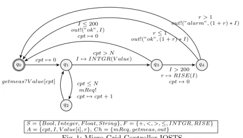
Example 1. Let us illustrate an example of IOSTS inspired from the Sesam-Grids project [12]: Figure 1 describes a simple model of a Microgrid, that is, a system of interconnected and distributed smart components (smartmeters, controller, ...) in connection with energy resources and energy consumption devices. Our ex-ample describes a simplified model of a controller inside a Microgrid. Electricity measurements are requested by a smart controller (mReq! action) and sent by a smart meter (getmeas?V alue[cpt]). N measurements are stored in the array V alue whose data can be accessed through variables of the form V alue[i] with i integer. Then, they are used by the controller to compute the total electricity consumption via an integral calculation (I 7→ IN T GR(V alue)) where IN T GR is an external function. If the overall consumption is greater than 200, then the function RISE (which is also an external function) is called to compute, ac-cording to the returned consumption I, a rate r that is added to the energy price. The new price ((1 + r) ∗ i) is sent to the actuator via the (out) channel, together with a message indicating whether the rise is normal (”ok”, if r <= 1) or should trigger a warning (”alarm”, if r > 1). Otherwise, if the consumption is lower than 200, an acknowledgment is sent (out!(”ok”, I)). In Figure 1, guards of the form t1 ≤ t2, t1 < t2, t1 > t2 or t1 ≥ t2 are concise representations of respectively t1≤ t2= >, t1< t2= >, t1> t2= > or t1≥ t2= >.
2.3 Symbolic execution of IOSTS
Symbolic execution (SE) consists in executing the IOST S with symbolic vari-ables rather than numerical values. SE gathers constraints (path condition) over such variables that characterize under which circumstances a particular execu-tion path is taken.
To store information concerning an execution, we use a set F r of so-called fresh variables with F r ∩ A = ∅ and structures called symbolic states. F r is an infinite set in which, whenever necessary, it is possible to take a variable not previously used. A symbolic state η is a tuple (q, π, λ) where: q (or q(η)) denotes the state in Q reached after an execution leading to η, π ∈ SenF(F r) (or π(η))
q0 q2 q1 q3 q4 cpt 7→ 0 I 7→ IN T GR(V alue) cpt > N cpt ≤ N mReq! cpt 7→ cpt + 1 getmeas?V alue[cpt] I ≤ 200 out!(”ok”, I) cpt 7→ 0 I > 200 r 7→ RISE(I) cpt 7→ 0 r > 1 out!(”alarm”, (1 + r) ∗ I) r ≤ 1 out!(”ok”, (1 + r) ∗ I)
S = {Bool, Integer, F loat, String}, F = {+, <, >, ≤, IN T GR, RISE} A = {cpt, I, V alue[i], r}, Ch = {mReq, getmeas, out}
Fig. 1: Micro Grid Controller IOSTS
is the path condition that should be satisfied for the execution to reach η and λ : A → TF(F r) (or λ(η)) denotes terms over variables in F r that are assigned to variables of A.
Definition 2 (SE of transitions). Let G = (Q, q0, T r) be an IOSTS, tr = (q, ψ, act, ρ, q0) a transition of T r and η = (q, π, λ) a symbolic state.
Let us define λias λ[x17→ f1, . . . , xn7→ fn] if act is of the form c?(x1, . . . , xn), where each fi is a fresh variable in F r and as λ otherwise. The symbolic ex-ecution SE(tr, η) of tr from η is the symbolic transition (η, λi(act), η0) where η0= (q0, π0, λ0), with π0= π ∧ λ(ψ), and λ0 = λi◦ ρ.
We denote F r(SE(tr, η)) the set of all fresh variables of F r occurring in its definition while not already present in η.
The symbolic execution tree associated with the IOST S is then defined sim-ply by executing all transitions from all symbolic states.
Definition 3 (SE of IOST S). Given an IOSTS G = (Q, q0, T r) over Γ = (A, Ch), the symbolic execution SE(G) = (SS, Init, ST ) of G is minimally de-fined by:
– Init = (q0, >, λ0) is the initial state. Init is in SS and we have ∀x ∈ A, λ0(x) ∈ F r, and ∀x 6= y ∈ A, λ0(x) 6= λ0(y). We denote F r0= {λ0(x) | x ∈ A} the set of variables used in Init.
– ST is a set of symbolic transitions such that for any η = (q, π, λ) in SS and for any tr ∈ T r of source state q, there exists one symbolic execution SE(tr, η) = (η, actF, η0) of tr from η with SE(tr, η) ∈ ST and η0 ∈ SS. Moreover F r(SE(tr, η)) ∩ F r0= ∅ and for any two distinct symbolic transitions SE(tr1, η1) and SE(tr2, η2) in ST , F r(SE(tr1, η1)) ∩ F r(SE(tr2, η2)) = ∅. For st = (η, actF, η0) in ST , we denote source(st) = η and target(st) = η0.
Now, we define paths of the symbolic tree resulting from the symbolic exe-cution of an IOST S:
Definition 4 (Symbolic Paths). The set P aths(SE(G)) of paths of SE(G) is the set of all sequences st1· · · stnwith ∀i ∈ 1..n, sti∈ ST such that source(st1) = Init and for any j < n, q(target(stj)) = q(source(stj+1)).
For a path δ = st1· · · stn with 1 ≤ n, we note End(δ) = target(stn) and F r(δ) = ∪i∈1..nF r(target(sti)). By convention, End(ε) = Init and F r(ε) = ∅.
By construction, path conditions accumulate constraints from all the guards of the IOSTS transitions over a path. Hence, feasibility of path pa is checked by calling a solver over the path condition of the last state of pa. In the sequel, such call will be denoted Sat(π(End(pa)).
As already mentioned in section 1, external functions such as IN T GR and RISE have no built-in interpretations in standard constraint solvers. Thus, when path conditions contain external functions, usual constraint solving techniques cannot be applied directly. We thus propose an improved resolution method to guide the symbolic execution by checking paths feasibility up to some function calls.
3
Function summaries
Instead of either considering external functions as purely abstract by replacing their output with a fresh variable or inserting their code (inlining) at model level quickly leading to combinatorial explosion, our approach allows to control this issue by replacing external functions with summaries that offer a partial and extendable view of the function within the model.
In the sequel, P will denote a distinguished subset of F , the set of all external functions.
3.1 Summaries
Values which are used to summarize an external function are taken from its concrete execution on some inputs. This can be represented and saved as a table mapping a finite set of tuples associating input and output data of the function. Notation 31 For p ∈ P an external function of profile s1. . . sn → sn+1 and pM ∈ M its interpretation, we denote by tab
p, a set of tuples (v1, . . . , vn, vn+1) ∈ Ms1× · · · × Msn× Msn+1 verifying pM(v1, . . . , vn) = vn+1, a function table of p. If tabp covers the entire domain of p then it will fully represent pM.
We associate with each external function a summary built on values in the function table. More precisely, a function call will be stored in a given symbolic state under the form
(p, (t1, · · · , tn), x)
indicating that a call has been performed for the external function p with argu-ments (t1, · · · , tn) and that its result is stored in the fresh variable x.
Definition 5 (Function call summaries). Let Cls ⊆ Calls(P ) be a set of function calls and T ab = (tabp)p∈P, where tabp is a function table associated to p in P .
The summary of Cls up to T ab is:
Sums(Cls, T ab) = ^
cl=(p,(t1,··· ,tn),x)∈Cls,
tabp∈T ab
Sum(cl, tabp)
where Sum(cl, tabp) computes the disjunction of different inputs/output tuples of tabp, i.e.: Sum(cl, tabp) = _ (v1,··· ,vn+1)∈tabp ((^ i≤n ti= vi) ∧ x = vn+1)
with the convention Sum(cl, ∅) = ⊥.
Example 2. Let us go back to the Microgrid example (Figure 1) with the hy-pothesis N = 2. Then, a scenario involves two measurements m1 and m2. For illustrative purposes, values that will be used in the summaries associated to the external functions IN T GR and RISE are given in Table 1. Based on the values provided by Table 1, we can then compute the corresponding summaries for the set of function calls Cls = {cl1, cl2} with cl1 = (IN T GR, ([m1, m2]), I) and cl2= (RISE, (I), r):
– Sum(cl1, tab(IN T GR)) is
(m1= 123 ∧ m2= 96 ∧ I = 228) ∨ (m1= 148 ∧ m2= 141 ∧ I = 300) – Sum(cl2, tab(RISE)) is
(I = 202 ∧ r = 0.7) ∨ (I = 300 ∧ r = 2.42)
Finally, Sums(Cls, T ab) is simply Sum(cl1, tab(IN T GR))∧Sum(cl2, tab(RISE))
tab(IN T GR) [123, 96] 228 [148, 141] 300 tab(RISE) 202 0.7 300 2.42
Table 1: IN T GR and RISE tables
3.2 Formula transformation
A path condition ϕ is built over terms of TF(V ) that may contain occurrences of external functions. Since the satisfiability of ϕ requires to find an interpretation ν ensuring M |=ν ϕ, the idea is to proceed in two steps:
1. ϕ is transformed into a formula with no occurrence of external functions and a set of function calls.
2. the satisfiability of ϕ is checked with a constraint solver and based on external function summaries (built on concrete executions of called functions).
For a formula ϕ containing a term of the form p(t1, · · · , tn) with p ∈ P , we will eliminate the occurrence of p in ϕ by introducing a new fresh variable x in charge of storing the result of the application of p to the terms t1, . . . , tn. An interpretation will be acceptable as a solution only if it evaluates terms t1, . . . , tn and x so that they correspond to one of the elements of the function table tabp. Thus, while eliminating all occurrences of external function in formulas, we also collect all tuples (t1, . . . , tn, x) memorizing all contexts of calls of external functions.
Let us first define a function χ : TF(V ) → TF(V ∪ F r) × Calls(P ) as follows: – if t is a variable or a constant3, χ(t) = (t, ∅)
– if t is of form f (t1, . . . , tn) with f 6∈ P , then4 χ(t) = (f (χ(t1)|1, . . . , χ(tn)|1), ∪i∈1..nχ(ti)|2) – if t is of form p(t1, . . . , tn) with p ∈ P , then
χ(t) = (x, {(p, (χ(t1)|1, . . . , χ(tn)|1), x)}∪i∈1..nχ(ti)|2) with x a fresh variable in F r.
We assume that all fresh variables introduced by function calls (i.e. the sets χ(t)|2) are pairwise disjoint. Note that the term substitution is performed itera-tively by starting with the innermost sub-terms in case of nested function calls. The function χ is canonically extended to formulas by preserving formula struc-ture and accumulating all sets of function calls in a unique set. In the sequel, for a formula ϕ, χ(ϕ)|1, the formula ϕ without external functions, will be denoted ϕ and χ(ϕ)|2, the set of associated calls, will be denoted κ(ϕ).
Example 3. Let us denote ϕ0the formula RISE(IN T GR([x+1, 0])) > 1 defined over the external functions IN T GR and RISE and the variable x.
Then, ϕ0 is r > 1 while κ(ϕ0) is {(RISE, (I), r), (IN T GR, ([x + 1, 0]), I)} with I and r new fresh variables.
Now that we are able to remove external functions, we will propose an algo-rithm to check formula satisfiability.
4
Satisfiability of formulas up to function summaries
Given a formula ϕ possibly built over external functions, we aim at defining an algorithm that analyzes the satisfiability of ϕ up to summaries of called external functions. Recall that ϕ is transformed into a formula (ϕ) with no occurrence of external functions, while we keep track of external function calls in κ(ϕ). We also suppose that we have function tables for these external function calls in T ab.
3
A constant is a function of profile of the form → s.
4
Since by construction Sums(κ(ϕ), T ab) is the formula specifying that func-tion calls of κ match with at least a tuple of T ab, if Sat(ϕ ∧ Sums(κ(ϕ), T ab)) returns a solution, then ϕ is satisfiable (i.e. there exists an interpretation ν such that M |=ν ϕ). Otherwise, either ϕ is not satisfiable (i.e. ∀ν, M 6|=ν ϕ) or ϕ is satisfiable but the function tables (used to summarize functions) are not com-plete enough to exhibit an interpretation ν such that M |=ν ϕ. Therefore, in the sequel we place ourselves in the hypothesis that function tables can be enriched during the satisfiability search. Furthermore, some heuristics are proposed to help the solver finding a solution when current function summaries are not com-patible with the formula, e.g. to find additional input data for external functions that could make the formula feasible. We describe these heuristics in more detail below.
4.1 Resolution strategies
NoCorres strategy: N oCorres computes a formula guaranteeing that the inputs of called external functions are different from those already present in the current function tables. This formula will be used later to get new inputs for the concrete executions of external functions, ensuring the enrichment of the function tables, which in turn increases chances to find a solution.
Definition 6 (NoCorres). Let Cls ⊆ Calls(P ) be a set of function calls and T ab = (tabp)p∈P a set of tables where tabp is the table associated to p in P . N oCorres(Cls, T ab) is defined as follows:
N oCorres(Cls, T ab) = _
cl=(p,(t1,··· ,tn),x)∈Cls,
tabp∈T ab
(N oCorres1(cl, tabp))
with N oCorres1((p, (t1, · · · , tn), x), tabp) being defined as follows:
^ (v1,··· ,vn+1)∈tabp
(_ i≤n
ti6= vi)
By considering the conjunction of N oCorres(κ(ϕ), T ab) and ϕ, the solver can-not compute interpretations of variables for which all function calls in κ(ϕ) are already present in T ab.
Example 4. By applying the above N oCorres definition on the set of func-tion calls and tables given in Example 2, N oCorres(Cls, T ab) is the formula N oCorres1(cl1, T ab(IN T GR)) ∨ N oCorres1(cl2, T ab(RISE)) where:
– N oCorres1(cl1, tab(IN T GR)) is
(m16= 123 ∨ m26= 96) ∧ (m16= 148 ∨ m26= 141) – N oCorres1(cl2, tab(RISE)) is (I 6= 202) ∧ (I 6= 300)
Dependency heuristic: Another way to accelerate and help the solver resolution task to find new inputs, when no solution is found with the current function tables, is to take advantage of direct dependencies between function calls. Indeed when the arguments of a call to an external function f depend on the result of calls to other external functions fi, we can indicate to the solver to search for solutions in which the inputs of f are compatible with the outputs already present in the tables of the fi.
Definition 7 (Dep). Let Cls ⊆ Calls(P ) be a set of function calls and T ab = (tabp)p∈P a set of tables where tabp is the function table associated to p in P .
Dep(Cls, T ab) is defined as follows: Dep(Cls, T ab) = ^
cl∈Cls
(Dep1(cl, Cls, T ab))
with Dep1(cl, Cls, T ab) being defined as follows: ^
cli=(q,(t01,··· ,t0n),x0)∈Depcl
(CorresRes(cli, tabq))
where:
– For cl = (p, (t1, · · · , tn), x), Depcl = {cli = (q, (t01, · · · , t0n), x0) ∈ Cls \ {cl} | x0 ∈ S
i≤nOcc(ti)} is the set of function calls on which the inputs of cl depend, i.e. the result of these function calls occurs in one or several input terms of cl.
– For cl0= (q, (t01, · · · , t0n), x0), CorresRes(cl0, tabq) is the formula _
(v1,··· ,vn+1)∈tabq
(x0= vn+1)
CorresRes(cl0, tabq) extracts values from the tables of function calls on which cl0 depends.
Example 5. Let us consider again the function calls introduced in Example 2. We have:
– Depcl2 = {cl1} with cl1 = (IN T GR, ([m1, m2]), I), because I (the variable storing the result of cl1) is an input of cl2= (RISE, (I), r).
– CorresRes(cl1, tab(IN T GR)) is (I = 228 ∨ I = 300)
Therefore, to find new inputs for RISE, we can give to the solver Dep(cl2, Cls), that is CorresRes(cl1, tab(IN T GR)) to exploit the values of I already existing in T ab(IN T GR).
By combining both N oCorres and Dep heuristics, it is possible to generate new sets of inputs, i.e. new rows in the tables of external functions that are relevant for the overall path constraint resolution. Indeed, N oCorres ensures that we will add at least one new row to a function table, while Dep takes care of avoiding solutions that cannot be satisfied by the current summaries of the callers, and are thus useless for the current solving process.
4.2 SolveTab algorithm
Algorithm 1 describes our dynamic solving procedure SolveT ab(m, ϕ, κ(ϕ), T ab). The goal of SolveT ab is to analyze the satisfiability up to some function tables T ab of a formula (ϕ) with no occurrences of external functions, provided with a set of function calls (κ(ϕ)). The integer parameter m is used to bound the number of attempts that are made to increase the size of function tables. As explained in the previous section, we resort to this mechanism when no tuple in a function table is compatible with ϕ. However, since there is no guarantee that extending function tables will eventually lead to find a solution for ϕ ∧ Sums(κ(ϕ), T ab), we cut the search after at most m steps. If no solution is found beyond m or no possible function inputs are found, then we can deduce that the formula is unsatisfiable up to function tables. The case m = 0 corresponds to a purely static version where a solution is searched without modifying function tables (i.e. T ab is then a static variable).
Algorithm 1: SolveT ab(m, ψ, κ, T ab)
Data: m: an integer, ψ: a formula without black-box functions, κ : a set of function calls, T ab: function tables
Result: satisfiability of ψ up to κ; T ab: updated function tables
1 begin
2 sol ← Sat(ψ ∧ Sums(κ, T ab));
3 T abM odif ied ← T rue;
4 while T abM odif ied and sol = N ON E and m 6= 0 do
5 In ← Sat(ψ ∧ NoCorres(κ, T ab) ∧ Dep(κ, T ab)) /* Search for new solutions while considering dependencies between function calls */ ;
6 if In = NONE then /* no possible inputs for function */
7 In ← Sat(ψ ∧ NoCorres(κ, T ab)) /* Search for new possible solutions without considering function dependencies */ ;
8 if In 6= NONE then /* new possible inputs for function */
9 for each call cl = (p, (t1, · · · , tn), x) in κ do
10 V Ins ← Ins(In, cl) /* extract inputs for p from In */;
11 r ← Execp(V Ins) /* concrete execution of p */;
12 T ab(p) ← (V Ins, r).T ab(p) /* save new tuple in T ab */;
13 sol ← Sat(ψ ∧ Sums(κ, T ab));
14 else
15 T abM odif ied ← F alse;
16 m ← m − 1;
17 return (sol, T ab);
Let us now give some few comments on Algorithm 1. By hypothesis, argu-ments (ψ, κ) = χ(ϕ) for some ϕ, so that ψ and κ share external functions and variables.
If Sat(ψ ∧Sums(κ, T ab)) gives back a result sol, then sol directly provides an interpretation of variables that satisfies the formula ϕ in which external functions are interpreted according to values given in their associated tables T ab. In other words, by construction M |=solϕ.
In case no solution is found with Sat(ψ ∧ Sums(κ, T ab)) in Line 2 (ψ is unsatisfiable up to current function summaries), then we try to find additional input data for external functions that could enrich T ab (and function summaries) and make the formula satisfiable. In order to guide the solver to find new inputs, Dep and N oCorres heuristics can be used. N oCorres is necessary to compute new inputs distinct from those already present in current tables (that failed to provide us with a solution). On the other hand, Dep is an alternative option that can facilitate the search for inputs that are compatible with dependencies among function calls. However, this might restrict the search space too much, as we may need to add a new output to the table of function f to find a suitable input for g that depends on f . Therefore, if adding the Dep condition results in an unsatisfiable formula (Line 7), we call the solver again with only the formula and the N oCorres condition. Indeed, the new tuples might give us new outputs that will in turn make Dep satisfiable at next step, or even give directly a solution to the original problem.
If an interpretation (variable In) is found, then lines 10, 11 and 12 allow us to add new tuples in function tables (variable T ab), by successively extracting input values V Ins ← ins(In, cl) for each function call (line 10), concretely executing the function (line 11) with V Ins as input data, (Execp being the reference implementation of p), to obtain the corresponding output (variable r) and finally storing new tuples in T abp (line 12). Then, the solver is called (line 13) to check the satisfiability of ψ, with the new summaries based on the enriched function tables.
Last, let us point out that a bigger number m of allowed attempts to search for new tuples enriching function tables gives more chances to find a solution, but will possibly take longer to compute.
4.3 Discussion: SolveT ab for symbolic execution
Since path conditions are formulas built over terms that may contain occurrences of external functions, we proceed as detailed in the previous section in order to check symbolic paths feasibility according to function summaries. For that, we use the SolveT ab solving Algorithm 1 based on concrete executions of called functions to guide the symbolic execution of IOST S. Therefore, we need to extend symbolic states by accumulating function calls. An extended symbolic state is of the form η = (q, π, λ, κ), where κ (or κ(η)) denotes the sequence of function calls of the form (p, (t1, · · · , tn), x). By construction, the path condition π does not contain occurrences of external functions.
A symbolic state (q, π, λ, κ) is satisfiable according to function summaries only if there exists an integer m and function tables T ab such that the result (sol, T ab) provided by SolveT ab(m, π, κ, T ab) defines an interpretation sol of fresh variables ensuring the interpretation of π as true.
The symbolic execution in accordance with function tables is based on the SolveT ab resolution algorithm which takes as arguments, in addition to the path condition and the set of accumulated function calls, the parameter m and the set of tables T ab. If we note SET ab,m(G) the symbolic execution of G using SolveT ab for building satisfiable symbolic states, then SET ab,m(G) is highly dependent on the initial tables (T ab) specifying called functions, the chosen threshold of resolution attempts m, the choice of the solver and the strategy of traversal (in depth, in width, . . . ) of the symbolic tree. Thus, the construction of SET ab,m(G) will more or less approach the ideal symbolic tree SE(G). If elements of T ab are representative enough of the behavior of called functions, with regard to the solicitations of the IOST S or if m is large enough to find a solution for each possible path of the IOST S (by enriching function tables), then SET ab(G) becomes closer to SE(G) and more states become reachable.
5
Implementation and Experiments
5.1 Implementation
DIVERSITY tool: DIVERSITY [3, 14], is a multi-purpose and customizable platform for formal analysis based on symbolic execution (test generation, proof, deadlock search, etc.) that is on its way to becoming an Eclipse open-source project5. DIVERSITY generates a symbolic tree (for a fixed maximal height) by simulating the system specification with input symbols rather than concrete values for data. Test inputs are computed by solving the path conditions. For that purpose, DIVERSITY integrates solvers such as Z36, and CV C47.
We have implemented the SolveT ab algorithm 1 and the heuristics described in Section 4 as additional Formal Analysis Module (FAM) for checking satisfia-bility of path conditions within DIVERSITY. By default, constraints involving external functions are left uninterpreted (i.e. out of the scope of solvers). In addition, variable assignments within an IOST S transition contain only basic operations. Now, all such external functions can be handled with the newly implemented technique, using values recorded in function tables. The SolveT ab algorithm allows to know whether a new execution context EC (a symbolic state) can be built in the symbolic execution tree in accordance with called functions, after the execution of a transition in the IOST S. In other words, it checks if a transition of the IOST S could be fired or not according to called functions, with a possible enrichment of the function tables. Therefore, thanks to SolveT ab we ensure the symbolic tree’s construction with only feasible paths compatible with called functions while ensuring a high transition coverage of the IOST S transitions. 5 https://projects.eclipse.org/proposals/eclipse-formal-modeling-project 6 https://z3.codeplex.com/ 7 http://cvc4.cs.nyu.edu/web/
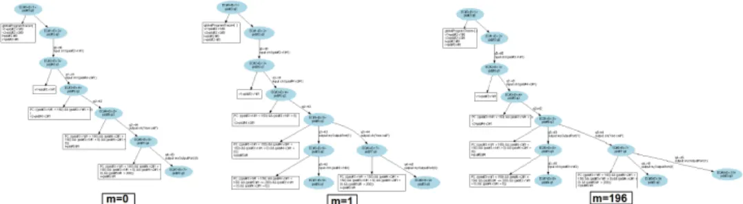
Microgrids case study: Here, we discuss the application of our technique to the Microgrid example 1 that uses external function calls (IN T GR and RISE). For that, we present the resulting symbolic trees (to a depth of 6) by applying the SolveT ab algorithm with the initial function tables 1 and various values of m, the number of attempts made to increase the function tables. At first, we use the static version (static tables, m = 0). Result is shown in the left tree of Figure 2. Then we progressively increase m until 196, function tables are enriched by concretely executing functions with new inputs found thanks to NoCorres and Dependency heuristics. As expected, this permits to cover more transitions of the model, reach more symbolic states and explore more feasible paths. Indeed the size of the generated tree grows with the value of m. The middle tree of figure 2 is obtained with m = 1, while the one on the right is the result of m = 196, where all transitions of the IOST S are covered.
Fig. 2: Symbolic execution tree in DIVERSITY
5.2 Experiments
A summary of the main outcomes of the application of our technique to the Microgrid example is provided in Table 2. It should be noted that our results are based on the initial function tables given in table 1 and that we dispose of the functions’ implementation in order to be able to execute them with appro-priate inputs in an unitary setting. For each experiment (i.e. each line), we fix ”m” (maximum number of attempts for the SolveT ab algorithm) and the maxi-mum ”height” allowed for the symbolic tree. Then we record results concerning the enriched tables (number of tuples) and the symbolic tree computation: the number of reachable states, the achieved IOST S transitions coverage and the execution time. Again, when m = 196 all possible symbolic states are covered, and there is no need to try to further enrich the function tables.
The resulting coverage rate and execution time depend on the initial function tables. In fact, the more the elements of called function tables are representative of the function behaviors and compatible with path conditions, the less attempts are needed to achieve the same level of coverage. For instance, if we now start with the initial function tables of table 3 for the Microgrid example, all transi-tions of the specification are covered (in 2s759ms) without doing any concrete
Micro-Grid IOSTS: initial Tab (Tables 1) ”m” height Enriched Tab states transition
coverage time INTGR RISE 0 15 2 2 16 62.5% 638ms 1 15 8 3 27 75% 2s 196 15 198 3 120 100% 4m15s
Table 2: Experiments with initial Tables 1
tab(IN T GR) [0, 0] 0 [12, 18] 30 [123, 96] 228 [148, 141] 300 tab(RISE) 202 0.7 228 0.97 300 2.42
Table 3: Other initial Tables
execution (m = 0), as all possible outcomes are captured by one row of the tables.
Micro-Grid IOSTS: other initial Tab (Tables 3) ”m” height Enriched Tab states coverage time
INTGR RISE
0 15 4 3 120 100% 2s759ms
Table 4: Experiments with other initial Tables 3
6
Related Work
IOSTS and symbolic execution have been used in many works [6, 10, 17] for different purposes. Until now standard solvers were not capable of dealing with functions occurring in path conditions. The usage of symbolic execution and path feasibility analysis are studied in [7,35] but this is limited to the analysis of functions themselves and does not take into consideration the impact of function calls on the feasibility of the whole system.
Our work borrows the idea of mixing symbolic execution with information obtained from instrumented concrete executions, from concolic testing, a method that has been implemented in various settings, such as [9, 18, 32]. However, these frameworks are primarily directed at source code level in the objective of unit testing. Another concolic tool, PathCrawler [36] proposed an approach to en-compass function calls [25], using pre/post-condition couples as a specification. Other unit testing frameworks traditionally use stubs [26], which are built manually in an ad-hoc way, to replace external functions for which no implemen-tation is available. Also, automatically-generated software stubs [19] are used for
abstracting (over-approximating) lower-level functions during dynamic test gen-eration [16] based on code.
[1,4,20,22], propose different techniques to conduct symbolic execution with simplified summary representations. But these techniques do not include heuris-tics similar to the ones (NoCorres, Dependency) we introduce in our paper.
Other techniques have been proposed to deal with constraints generated from symbolic code execution [2,30]. These techniques fall back on concrete values and use randomization to help simplify complex constraints that cannot be solved directly. Our approach based on IOSTS models is orthogonal to these code-based approaches and uses some heuristic search to solve path conditions including external function calls.
In our previous work [8], like in the work [25], we specify external functions by means of contracts (instead of tables): we unfolded the symbolic tree of an IOSTS by replacing each transition including an external function call by as many transitions as there are behaviors in the contract associated to the consid-ered external function.
7
Conclusion and future work
In this work, we use the IOSTS framework extended with external functions. We adapt existing symbolic execution techniques over IOSTS to deal with such function calls, using function tables to summarize them with a formula. The construction of a symbolic execution tree is based on an algorithm SolveT ab that permits to check path conditions satisfiability up to function summaries with the possibility of enriching function tables by concretely executing them, in order to achieve a high transition coverage of the IOST S.
The proposed approach has been implemented within the DIVERSITY sym-bolic execution tool. The results show that symsym-bolic execution coupled with func-tion summaries is a practical and effective approach to take into considerafunc-tion external functions for IOSTS models analysis mainly for model-based testing which is a significant motivation for our work. Nevertheless, it could probably be applied to other families of transition systems like those in [31, 33, 34].
References
1. Saswat Anand, Patrice Godefroid, and Nikolai Tillmann. Demand-driven compo-sitional symbolic execution. In Proceedings of the Theory and Practice of Software, 14th International Conference on Tools and Algorithms for the Construction and Analysis of Systems, pages 367–381, Berlin, Heidelberg, 2008. Springer-Verlag. 2. Saswat Anand, Corina S. P˘as˘areanu, and Willem Visser. Jpf-se: A symbolic
execu-tion extension to java pathfinder. In Proceedings of the 13th Internaexecu-tional Confer-ence on Tools and Algorithms for the Construction and Analysis of Systems, pages 134–138, Berlin, Heidelberg, 2007. Springer-Verlag.
3. Mathilde Arnaud, Boutheina Bannour, and Arnault Lapitre. An illustrative use case of the diversity platform based on uml interaction scenarios. Electron. Notes Theor. Comput. Sci., pages 21–34, 2016.
4. Domagoj Babic and Alan J. Hu. Structural abstraction of software verification conditions. In Proceedings of the 19th International Conference on Computer Aided Verification, pages 366–378, Berlin, Heidelberg, 2007. Springer-Verlag.
5. Boutheina Bannour, Jose Pablo Escobedo, Christophe Gaston, and Pascale Le Gall. Off-line test case generation for timed symbolic model-based conformance testing. In Testing Software and Systems, pages 119–135. Springer, 2012.
6. Boutheina Bannour, Christophe Gaston, Marc Aiguier, and Arnault Lapitre. Re-sults for compositional timed testing. In 20th Asia-Pacific Software Engineering Conference, APSEC, pages 559–564. IEEE Computer Society, 2013.
7. N. Bjørner, N. Tillmann, and A. Voronkov. Path feasibility analysis for string-manipulating programs. In TACAS, volume 5505 of LNCS. Springer, 2009. 8. Imen Boudhiba, Christophe Gaston, Pascale Le Gall, and Virgile Prevosto.
Model-based testing from input output symbolic transition systems enriched by program calls and contracts. In Testing Software and Systems - 27th IFIP WG 6.1 Inter-national Conference, ICTSS, volume 9447 of Lecture Notes in Computer Science, pages 35–51. Springer, 2015.
9. Cristian Cadar and Dawson Engler. Execution generated test cases: How to make systems code crash itself. Software Model Checking (SPIN), 2005.
10. James C.King. Symbolic execution and program testing. Communication ACM, 19:385–394, 1976.
11. Lori A Clarke. A system to generate test data and symbolically execute programs. IEEE Trans. Softw. Eng., pages 215–222, 1976.
12. The consortium Sesam-Grids. The Sesam-Grids Project. In http://www.sesam-grids.org/.
13. CREST. https://code.google.com/archive/p/crest/. Accessed: 2017-03-04. 14. J. Deltour, A. Faivre, E. Gaudin, and A. Lapitre. Model-based testing: An approach
with SDL/RTDS and DIVERSITY. In SAM, volume 8769 of LNCS. Springer, 2014.
15. DIVERSITY. https://projects.eclipse.org/proposals/
eclipse-formal-modeling-project. Accessed: 2017-03-04.
16. Dawson Engler and Daniel Dunbar. Under-constrained execution: Making auto-matic code destruction easy and scalable. In Proceedings of the 2007 International Symposium on Software Testing and Analysis, pages 1–4, New York, NY, USA, 2007. ACM.
17. Christophe Gaston, Pascale Le Gall, Nicolas Rapin, and Assia Touil. Symbolic execution techniques for test purpose definition. In Testing of Communicating Systems, pages 1–18. Springer, 2006.
18. Patrice Godefroid, Nils Klarlund, and Koushik Sen. Dart: Directed automated random testing. PLDI 05 Programming Language Design and Implementation, pages 213–223, 2005.
19. Patrice Godefroid, Nils Klarlund, and Koushik Sen. Dart: Directed automated random testing. SIGPLAN Not., pages 213–223, 2005.
20. Denis Gopan and Thomas Reps. Low-level library analysis and summarization. In Proceedings of the 19th International Conference on Computer Aided Verification, pages 68–81, Berlin, Heidelberg, 2007. Springer-Verlag.
21. jCUTE. http://osl.cs.illinois.edu/software/jcute/. Accessed: 2017-03-04. 22. Sarfraz Khurshid and Yuk Lai Suen. Generalizing symbolic execution to library
classes. SIGSOFT Softw. Eng. Notes, pages 103–110, 2005.
23. Nicolas Kicillof, Wolfgang Grieskamp, Nikolai Tillmann, and Victor Braberman. Achieving both model and code coverage with automated gray-box testing. In Advances in Model-Based Testing (A-MOST). ACM, 2007.
24. MathWorks. The Simulink documentation. In http://fr.mathworks.com/help/simulink/.
25. Patricia Mouy, Bruno Marre, Nicky Willams, and Pascale Le Gall. Generation of all-paths unit test with function calls. International Conference On Software Testing (ICST), pages 32 –41, 2008.
26. Glenford J. Myers, Corey Sandlers, and Tom Badgett. The Art of Software Testing. John Wiley & Sons, 3 edition, 2011.
27. Object Management Group. The UML standard specification. In http://www.omg.org/spec/UML/2.4.1/.
28. PathCrawler. http://frama-c.com/pathcrawler.html. Accessed: 2017-03-04. 29. Symbolic PathFinder. http://babelfish.arc.nasa.gov/trac/jpf/wiki/
projects/jpf-symbc. Accessed: 2017-03-04.
30. Corina S. P˘as˘areanu, Neha Rungta, and Willem Visser. Symbolic execution with mixed concrete-symbolic solving. In Proceedings of the 2011 International Sympo-sium on Software Testing and Analysis, pages 34–44, New York, NY, USA, 2011. ACM.
31. J. J.M.M. Rutten. A calculus of transition systems (towards universal coalgebra). Technical report, CWI (Centre for Mathematics and Computer Science), Amster-dam, The Netherlands, The Netherlands, 1995.
32. Koushik Sen, Darko Marinov, and Gul Agha. CUTE: A concolic unit testing engine for C. SIGSOFT Softw. Eng. Notes, 30:263–272, 2005.
33. Jan Tretmans. Conformance testing with labelled transition systems: Implementa-tion relaImplementa-tions and test generaImplementa-tion. Computer networks and ISDN systems, 29(1):49– 79, 1996.
34. Jan Tretmans. Model based testing with labelled transition systems. In Robert M. Hierons, Jonathan P. Bowen, and Mark Harman, editors, Formal Methods and Testing, pages 1–38. Springer-Verlag, Berlin, Heidelberg, 2008.
35. Y. Wang, Y. Xing, and X. Zhang. A method of path feasibility judgment based on symbolic execution and range analysis. International Journal of Future Generation Communication and Networking, 2014.
36. Nicky Williams, Bruno Marre, Patricia Mouy, and Muriel Roger. PathCrawler: automatic generation of path tests by combining static and dynamic analysis. Eu-ropean Dependable Computing Conference, pages 281–292, 2005.
![Table 2: Experiments with initial Tables 1 tab(IN T GR) [0, 0] 0 [12, 18] 30 [123, 96] 228 [148, 141] 300 tab(RISE)2020.72280.973002.42 Table 3: Other initial Tables](https://thumb-eu.123doks.com/thumbv2/123doknet/12943849.375292/16.918.270.661.171.420/table-experiments-initial-tables-rise-table-initial-tables.webp)
