HAL Id: hal-00821946
https://hal.inria.fr/hal-00821946
Submitted on 13 May 2013
HAL is a multi-disciplinary open access
archive for the deposit and dissemination of
sci-entific research documents, whether they are
pub-lished or not. The documents may come from
teaching and research institutions in France or
abroad, or from public or private research centers.
L’archive ouverte pluridisciplinaire HAL, est
destinée au dépôt et à la diffusion de documents
scientifiques de niveau recherche, publiés ou non,
émanant des établissements d’enseignement et de
recherche français ou étrangers, des laboratoires
publics ou privés.
HRF estimation improves sensitivity of fMRI encoding
and decoding models
Fabian Pedregosa, Michael Eickenberg, Bertrand Thirion, Alexandre Gramfort
To cite this version:
Fabian Pedregosa, Michael Eickenberg, Bertrand Thirion, Alexandre Gramfort. HRF estimation
im-proves sensitivity of fMRI encoding and decoding models. 3nd International Workshop on Pattern
Recognition in NeuroImaging, Jun 2013, Philadelphia, United States. �hal-00821946�
HRF estimation improves sensitivity of fMRI
encoding and decoding models
Fabian Pedregosa
∗†‡§, Michael Eickenberg
∗† ‡, Bertrand Thirion
†‡and Alexandre Gramfort
¶‡†Parietal Team, INRIA Saclay-ˆIle-de-France, Saclay, France ‡ CEA, DSV, I2BM, Neurospin bˆat 145, 91191 Gif-Sur-Yvette, France
§ SIERRA Team, INRIA Paris - Rocquencourt, Paris, France ¶ Institut Mines-T´el´ecom, T´el´ecom ParisTech, CNRS LTCI, Paris, France
Abstract—Extracting activation patterns from functional Mag-netic Resonance Images (fMRI) datasets remains challenging in rapid-event designs due to the inherent delay of blood oxygen level-dependent (BOLD) signal. The general linear model (GLM) allows to estimate the activation from a design matrix and a fixed hemodynamic response function (HRF). However, the HRF is known to vary substantially between subjects and brain regions. In this paper, we propose a model for jointly estimating the hemodynamic response function (HRF) and the activation patterns via a low-rank representation of task effects. This model is based on the linearity assumption behind the GLM and can be computed using standard gradient-based solvers. We use the activation patterns computed by our model as input data for encoding and decoding studies and report performance improvement in both settings.
Index Terms—fMRI; hemodynamic; HRF; GLM; BOLD; en-coding; decoding
I. INTRODUCTION
The use of decoding models [1] to predict the cognitive state of a subject during task performance has become a popular analysis approach for fMRI studies. The converse approach is the voxel-based encoding model, which describes the information about the stimulus or task that is represented in the activity of a single voxel [2].
The input to both types of analysis consists of activation pat-terns corresponding to different tasks or stimulus types. These activation patterns are straightforward to calculate for blocked trials or slow-event designs, but for rapid-event designs the evoked BOLD response for adjacent trials will overlap in time, complicating the identification task.
The general linear model (GLM) was proposed [3] to over-come this difficulty. It estimates the activation patterns evoked by separate events and allows for rapid-event settings. The GLM relies on a known form of the hemodynamic response function (HRF) to estimate the activation pattern. However, it is known [4] that the shape of this response function can vary substantially across subjects and brain regions.
In this study we propose to learn the specific form of the HRF in each brain voxel to improve the computation of the activation vectors in the GLM. Joint estimation of HRF and activation patterns has already been proposed in the literature, both within the frequentist [5] and Bayesian framework [6].
* both authors contributed equally
We propose a model based on the linearity assumption behind GLM and low-rank factorization. We are interested in assess-ing the impact on higher-level analysis such as encodassess-ing and decoding studies. In particular, we examine whether encoding and decoding models give significantly different results when the activation patterns used as input data are computed using this joint estimation method.
Notation: k · k denotes the euclidean norm for vectors. I denotes the identity matrix and ei denotes its ith column
vector. ⊗ denotes the Kronecker product and vec(A) denotes the concatenation of the columns of a matrix A into a single column vector.
II. HRFESTIMATION VIA LOW-RANK APPROXIMATION We denote the observed fMRI time series for a single voxel by y = (y1, . . . , yn) where yiis the measurement at time iTR,
with TR being the time of repetition and n is the number of scans within the session. As reference HRF we use the one described by Glover [7], and denote it by hc. In this case, the
GLM model specifies the observed BOLD signal as:
y = Xhcβ + P w + ε , (1)
where Xhc ∈ R
n×pis the design matrix, i.e. the matrix whose
columns are a discrete convolution of hc with the binary
stimulus vector Vi for condition i, P ∈ Rn×q is the matrix of
confounds (drifts, motions etc.) and ε ∈ Rn is the vector of
residuals, which is modeled as an auto-regressive process of order 1 (AR1(1)) to take into account the temporal correlations in the noise. We now define the binary matrix ˜X ∈ Rn×pr as
˜ X = r X k=0 Lk(V ⊗ eTk) (2)
where r is the duration of the HRF in multiples of TR, V the binary stimulus matrix and Lk is the lower shift matrix
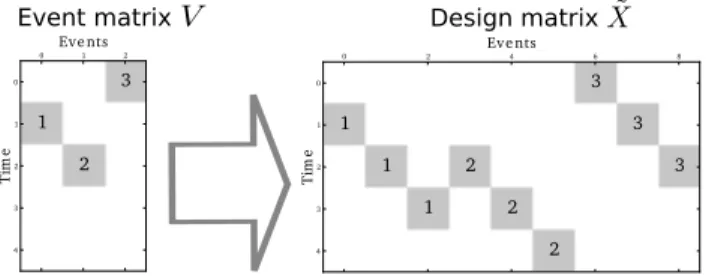
of order k, i.e. the matrix that shifts downwards k places all elements. Figure 1 illustrates the relationship between the event matrix and the design matrix. Matrix ˜X has the property that ˜X vec (hβT) = X
hβ, for any vector h, allowing us to
write equation (1) with an explicit linear dependency on h, y = ˜X vec(hcβT) + P w + ε.
Event matrix Design matrix 0 1 2 0 1 2 3 4 T im e 1 2 3 Eve nts 0 2 4 6 8 0 1 2 3 4 T im e 1 1 1 2 2 2 3 3 3 Eve nts
Fig. 1. Design matrix for Finite Impulse Response models. Different numbers correspond to different events. Here the HRF is assumed to span over a period of 3 TRs.
The model parameters are then estimated such that they minimize the decorrelated residuals. Equivalently, we solve the following optimization problem for β, h and w:
arg min β,h,w 1 2kZ T(y − ˜X vec(hβT) − P w)k2 , (3)
where ZT is the whitening matrix associated with the AR(1)
covariance matrix estimated by maximum likelihood. This represents a linear regression model where the coefficients are the vectorization of a rank-one matrix. It can also be seen as a Finite Impulse Response (FIR) basis GLM with a constraint such that the HRF h is repeated for each condition. We will refer to this as the rank-one regression model. Note that while it is possible to add a regularization term to reflect prior knowledge of the shape of the HRF, no specific form of h is privileged within this model.
A. Choice of a particular basis
In certain cases it may be desirable to reduce the number of free parameters of the HRF function within the rank-one model. An effective technique consists in constraining h to be obtained as a linear combination of t basis functions with t ≤ r, in an approriately chosen basis. Common bases used to express the HRF include the Fourier basis, polynomial basis and the canonical HRF together with its derivatives up to a certain order.
Given the subspace generated by the columns of a matrix Q ∈ Rr×t, we impose h to lie in that subspace. In that case we
can write h = Qα for some α ∈ Rt. By the properties of the
Kronecker product we have the equivalence ˜X vec(QαβT) =
˜
X(I ⊗ Q) vec(αβT). We can now define our rank-one model
over parameters α instead of h by defining the design matrix ˜
XQ=P t
k=0Lk(V ⊗ qkT) where qi denotes the ith column of
Q.
B. Asynchronous design
When the events are not a multiple of the repetition time, constructing the design matrix ˜X cannot be accomplished directly by equation (2).
Let V represent the binary stimulus where the events are truncated to the closest TR. Furthermore, let V = Pm
i=0Ei,
where Eiis the matrix of individual events. In the case where
a continuous basis for the HRF is chosen this can be evaluated at all time. That is, the design matrix can be written as
˜ X = m X i=0 t X k=0 Lk(Ei⊗ qk,i)
where qk,i represents the kth vector in the basis evaluated
at the TR timepoints plus an offset equal to the offset of event i with respect to the TR.
C. Algorithm
Although the problem 3 is not convex, the cost function is differentiable and gradient-based methods can be used to solve the optimization problem. We used the limited-memory BFGS algorithm [8] to simultaneously optimize over parameters β, h, w. For simplicity, we have taken Z to be the identity. For the general result, simply multiply X, y, P by ZT. Popular
implementations of the algorithm only need as parameters the objective function (3) and the gradient, given by:
∇β=(I ⊗ hT) ˜XT( ˜X vec(hβT) + P w − y)
∇h=(βT ⊗ I) ˜XT( ˜X vec(hβT) + P w − y)
∇w=PT( ˜X vec(hβT) + P w − y)
The full gradient now can be computed by stacking ∇β, ∇h
and ∇w into a single vector. Since in this algorithm only
a matrix-vector product is used, the use of Kronecker prod-uct identities avoids the explicit creation of most Kronecker product matrices. We have found this implementation to take around 3 hours to perform a full brain analysis (124.000 voxels, 46 conditions) on commodity hardware with almost no increase in memory consumption once the data was loaded in memory. An implementation by the authors is publicly available1
III. VALIDATION
We use two fMRI datasets (one for encoding, one for decoding), and for each we consider two validation criteria. The first criterion is common to both datasets and assesses whether the learned HRF fits better unseen data than the canonical function. We fit a rank-one regression model on all but one session. This gives us an estimate of the HRF for all voxels. We then use this HRF to compute the log-likelihood of a GLM model on unseen data. In similar fashion, we compute the log-likelihood using the canonical HRF. A paired test allows us to conclude whether both likelihoods are significantly different and thus if one model has better goodness of fit.
This criterion serves to validate our model using a likelihood function defined on the raw fMRI timeseries. However, we are mainly interested in the GLM as a pre processing step for higher level analysis such as decoding or encoding models. That is why, in order to fully assess the relevance of this contribution, we propose to quantify the performance of our rank-one model using the performance metrics commonly used with decoding and encoding models.
0 5 10 15
Time (seconds)
0.2 0.0 0.2 0.4 0.6 0.8 1.0 1.2 estimated (with std deviation) canonical HRF 0 5 10 15Time (seconds)
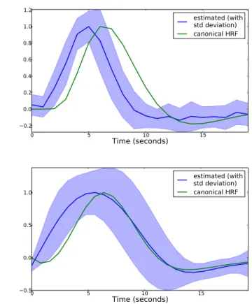
0.5 0.0 0.5 1.0 estimated (with std deviation) canonical HRFFig. 2. Estimated HRF for the two different datasets, using the top 100 performing voxels. In blue we show the mean HRF across these voxels, together with its standard deviation in more transparent color. For the first image, the HRF was expressed using a FIR basis with 20 degrees of freedom. For the second images, a basis of 6 elements consisting on the canonical HRF and its five succesive derivatives was chosen.
A. Data description
Natural imagesFor the encoding model, we use the publicly available dataset from [9], where the task consists in predicting the activation maps from a set of natural images. Subjects viewed 1750 training images, each presented twice, and 120 validation images, each presented 10 times, while fixating a central cross. Images were flashed 3 times per second (200ms on-off-on-off-on) for one second every 4 seconds, leading to a rapid event-related design. The data was acquired in 5 scanner sessions, each comprising 5 blocks of 70 training images, each presented twice within the block and 2 blocks of validation images showing 12 images each 10 times.
Evaluation of the performance of our GLM was done with a simple encoding task: Using a spatially smoothed Gabor pyramid transform modulus with 2 orientations and 4 scales, we used Ridge regression to learn a predictor of voxel activity on 80% (4 of 5 sessions, i.e. 1400 images) of the training set. Linear predictions on the left out fold were compared to the true activations in l2 norm and normalized by the variance of
the voxel activity, before being subtracted from 1 (predictive r2 scoring).
Word decoding For the decoding task, we use the dataset described in [10], where the task consist in predicting the
visual percept formed by four letter words. Each word was presented on the screen for 3 s at a flickering frequency of 15 Hz. A 5 s rest interval was inserted between each word presentation. The subject was asked to fixate a colored cross at the center of the screen. Each session comprised 46 words including 6 verbs. To ensure that subjects were reading, they were asked to report with a button press when a verb was presented on the screen. Repetitions corresponding to verbs were then removed from the analysis. Six acquisition blocks were recorded, leading to 240 different words used in the analysis. We evaluate the performance of our GLM in this decoding task by calculating the percentage of overall correctly predicted bars forming the image.
B. Results
We first report results on the natural images dataset. As described above, we validate by fitting a rank-one regression model on all but one session. On the left-out session, we found the log-likelihood of the GLM model obtained with the data-driven HRF to be consistently larger than the log-likelihood obtained using a canonical HRF. A paired difference test was used to conclude that the mean likelihood of the rank-one model is significantly larger with p-value < 10−3.
The estimated HRF across the 100 most responding vox-els is presented in Fig. 2. We show the average value for the learned HRFs across voxels together with its standard deviation. As expected, the data-driven HRFs resemble the canonical HRF, however, the peak is located on average one second before the peak of the canonical function.
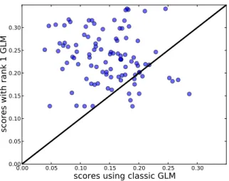
The predictive r2scores of 100 voxels are shown in a scatter
plot in Fig. 3. We chose the 100 best predicted voxels using a classic GLM. These scores are on the x-axis. The y-axis shows the scores using our method. Significantly more scores lie above the diagonal (p < 10−4), Wilcoxon signed rank test), suggesting that that learning the HRF is beneficial to this encoding scheme.
The second dataset that we analyze is the word-decoding dataset. This dataset is an asynchronous setting with TR = 2.4 s and trials of 8 s. As described above we chose to oversample by a factor or 3 the original TR to a TR of 0.8s. Because of the low time resolution and the shorter time course, we chose to constrain the HRF to a small subspace in order to avoid overfitting associated with complex models. The set of basis functions for this subspace is given by the canonical HRF and its five successive derivatives. We have experimented with several different bases including Chebyshev polynomials, Fourier basis and discrete cosine basis. All these basis capture the general trend of the HRF function and give similar results, but each set induces some bias towards specific shape functions, while this set of generators favors more biologically plausible models. As with the previous dataset, we observed log-likelihood values that are constantly larger than for the GLM. A paired difference test was used to conclude that the mean log-likelihood is significantly higher with p-value < 3 × 10⁻³.
0.00 0.05 0.10 0.15 0.20 0.25 0.30
scores using classic GLM
0.00 0.05 0.10 0.15 0.20 0.25 0.30
scores with rank 1 GLM
Fig. 3. Performance scores of individual voxels using the rank-one model against the performance obtained by a standard GLM. Elements over the diagonal represent voxels in which our model obtained higher scores.
As can be seen in Fig. 2 second image, the estimated HRF resembles the canonical HRF, which is not surprising given the subspace in which it is constrained. As with the previous dataset, the peak of the HRF is slightly advanced with respect to the canonical function.
We used the activation patterns estimated by the rank-one regression model as input to the decoding study. Within the four subjects analyzed, we observed a systematic increase in the mean score, ranging for +1% to +3% (out of a score of 65%). We observed higher increase for the best performing subjects. A Wilcoxon signed-rank test on the scores across subjects gave us a p-value < 0.07 for the significance of these differences.
IV. CONCLUSION
We have presented a model that jointly estimates the hemo-dynamic response function (HRF) and the activation patterns from the BOLD signal. This model, named rank-one regres-sion, can be optimized using standard smooth optimization methods such as L-BFGS. We investigated whether this model yields better prediction for encoding and decoding models.
In a first step, we assessed the quality of the HRF estimation by comparing the likelihood of the GLM on unseen data using both the estimated HRF and the canonical HRF. To assess the impact on encoding and encoding models, we have selected two fMRI datasets and used the GLM coefficients obtained by our rank-one model as input data.
We found out that using the activation patterns estimated by the rank-one model significatively improved encoding and de-coding studies. In the ende-coding study we found a generalized improvement across voxels. In the decoding study observed improved scores for all subjects across the study.
V. ACKNOWLEDGMENT
This work was supported by grants IRMGroup ANR-10-BLAN-0126-02 and BrainPedia ANR-10-JCJC 1408-01. The
authors would like to thank Guillaume Obozinski, Francis Bach and Philippe Ciuciu for fruitful discussions.
REFERENCES
[1] J.-D. Haynes and G. Rees, “Decoding mental states from brain activity in humans,” Nature Reviews Neuroscience, vol. 7, no. 7, pp. 523–534, 2006.
[2] T. Naselaris, K. N. Kay, S. Nishimoto, and J. L. Gallant, “Encoding and decoding in fMRI,” Neuroimage, vol. 56, no. 2, pp. 400–410, 2011. [3] K. J. Friston, A. P. Holmes, K. J. Worsley, J.-P. Poline, C. D. Frith, and
R. S. Frackowiak, “Statistical parametric maps in functional imaging: a general linear approach,” Human brain mapping, vol. 2, no. 4, pp. 189–210, 1994.
[4] D. A. Handwerker, J. M. Ollinger, M. D’Esposito et al., “Variation of BOLD hemodynamic responses across subjects and brain regions and their effects on statistical analyses,” Neuroimage, vol. 21, no. 4, pp. 1639–1651, 2004.
[5] S. Donnet, M. Lavielle, and J.-B. Poline, “Are fmri event-related response constant in time? a model selection answer,” Neuroimage, vol. 31, no. 3, pp. 1169–1176, 2006.
[6] S. Makni, P. Ciuciu, J. Idier, and J.-B. Poline, “Joint detection-estimation of brain activity in functional mri: a multichannel deconvolution so-lution,” Signal Processing, IEEE Transactions on, vol. 53, no. 9, pp. 3488–3502, 2005.
[7] G. H. Glover, “Deconvolution of impulse response in event-related BOLD fMRI,” Neuroimage, vol. 9, no. 4, pp. 416–429, 1999. [8] D. C. Liu and J. Nocedal, “On the limited memory method for large
scale optimization,” Mathematical Programming B, vol. 45, no. 3, pp. 503–528, 1989.
[9] K. N. Kay, T. Naselaris, R. J. Prenger, and J. L. Gallant, “Identifying natural images from human brain activity,” Nature, vol. 452, no. 7185, pp. 352–355, 2008.
[10] A. Gramfort, C. Pallier, G. Varoquaux, and B. Thirion, “Decoding visual percepts induced by word reading with fMRI,” in Pattern Recognition in NeuroImaging (PRNI), 2012 International Workshop on, Londres, Royaume-Uni, Jul 2012, pp. 13–16.