On the Neutrality of Flowshop Scheduling Fitness Landscapes

HAL Id: hal-00550356

https://hal.archives-ouvertes.fr/hal-00550356

Submitted on 18 Jul 2012

HAL is a multi-disciplinary open access

archive for the deposit and dissemination of

sci-entific research documents, whether they are

pub-lished or not. The documents may come from

teaching and research institutions in France or

abroad, or from public or private research centers.

L’archive ouverte pluridisciplinaire HAL, est

destinée au dépôt et à la diffusion de documents

scientifiques de niveau recherche, publiés ou non,

émanant des établissements d’enseignement et de

recherche français ou étrangers, des laboratoires

publics ou privés.

On the Neutrality of Flowshop Scheduling Fitness

Landscapes

Marie-Eleonore Marmion, Clarisse Dhaenens, Laetitia Jourdan, Arnaud

Liefooghe, Sébastien Verel

To cite this version:

Marie-Eleonore Marmion, Clarisse Dhaenens, Laetitia Jourdan, Arnaud Liefooghe, Sébastien Verel.

On the Neutrality of Flowshop Scheduling Fitness Landscapes. Learning and Intelligent OptimizatioN

Conference (LION 5), Jan 2011, Rome, Italy. pp.238–252, �10.1007/978-3-642-25566-3_18�.

�hal-00550356�

On the Neutrality of

Flowshop Scheduling Fitness Landscapes

Marie-El´eonore Marmion1,2_{, Clarisse Dhaenens}1,2_{, Laetitia Jourdan}1_,

Arnaud Liefooghe1,2_{, and S´ebastien Verel}1,3

1

INRIA Lille-Nord Europe, France

2

Universit´e Lille 1, LIFL – CNRS, France

3

University of Nice Sophia Antipolis – CNRS, France marie-eleonore.marmion@inria.fr, clarisse.dhaenens@lifl.fr, laetitia.jourdan@inria.fr, arnaud.liefooghe@univ-lille1.fr,

verel@i3s.unice.fr

Abstract. Solving efficiently complex problems using metaheuristics, and in particular local search algorithms, requires incorporating knowl-edge about the problem to solve. In this paper, the permutation flowshop problem is studied. It is well known that in such problems, several so-lutions may have the same fitness value. As this neutrality property is an important issue, it should be taken into account during the design of search methods. Then, in the context of the permutation flowshop, a deep landscape analysis focused on the neutrality property is driven and propositions on the way to use this neutrality in order to guide the search efficiently are given.

1

Motivations

Scheduling problems form one of the most important class of combinatorial op-timization problems. They arise in situations where a set of operations (tasks) have to be performed on a set of resources (machines), optimizing a given quality criterion. Flowshop problems constitute a special case of scheduling problems in which an operation must pass through all the set of resources before being com-pleted. Such scheduling problems are often difficult to solve, because of the large search space they induce, and then represent a great challenge for combinato-rial optimization. Therefore many optimization methods have been proposed so far and experimented on a set of widely-used benchmark instances. Regarding, the minimization of makespan in flowshop problems, iterated local search (ILS) approaches seem to achieve very good performance. In particular, St¨utzle’s ILS [1] stays one of the references of the literature. It has been listed as one of the best performing metaheuristics on a review of heuristic approaches for the flow-shop problem investigated in the paper [2]. More recently, Ruiz and St¨utzle [3] have proposed an iterated greedy algorithm to solve the flowshop problem, based on similar mechanisms, and they have shown that is outperforms the classical metaheuristics for this problem.

The aim of the paper is to analyze characteristics of the flowshop problems in order to understand and to explain why St¨utzle’s method achieves such good performance. A quick analysis shows that the neutrality is high in those problems and we want to explain how this neutrality influences the behavior of heuristic methods. It will then become possible to propose mechanisms that are able to exploit this neutrality.

The method proposed by St¨utzle consists of an Iterated Local Search (ILS) approach based on the insertion neighborhood operator. This operator is argued to be the best one by the original author, as it produces better results than the transpose operator, for example, while allowing a faster evaluation compared to the exchange operator. The method starts from a solution constructed using a greedy heuristic (the NEH heuristic), initially proposed by Nawaz et al. [4]. Next, the local search algorithm, based on a first improvement exploration of the neighborhood, is iterated until a local minimum is reached. Then, between each local search, a small perturbation is applied on the current solution using random applications of the transpose and exchange neighborhood operators. An important characteristic of this approach is the acceptance criterion of the ILS algorithm, which is based on the Metropolis condition (as in simulated anneal-ing). Indeed, such a condition allows to accept a solution with a same or worse fitness value than the current one.

Hence, the contributions of this work are the following ones. On the one hand, the specific problem of flowshop scheduling is deeply studied in terms of landscape analysis and neutrality. On the other hand, some propositions are drawn in order to exploit neutrality in the design of a local search algorithm. Of course, these considerations are still valid for other combinatorial optimization problems with a neutrality.

The paper is organized as follows. Section 2 is dedicated to the presentation of the flowshop scheduling problem investigated in this paper, and of the required notions about neutrality analysis in fitness landscapes. Section 3 presents the neutral networks analysis for the permutation flowshop problem under study, whereas Section 4 gives some hints on how to exploit the neutrality property in order to solve such problems efficiently by means of local search algorithms. Finally, the last section is devoted to discussion and future works.

2

Background

2.1 Definition of the Permutation Flowshop Scheduling Problem The Flowshop Scheduling Problem (FSP) is one of the most investigated schedul-ing problem from the literature. The problem consists in schedulschedul-ing N jobs {J1, J2, . . . , JN} on M machines {M1, M2, . . . , MM}. Machines are critical

re-sources, i.e. two jobs cannot be assigned to the same machine at the same time. A job Jiis composed of M tasks {ti1, ti2, . . . , tiM}, where tijis the jthtask of Ji,

requiring machine Mj. A processing time pij is associated with each task tij. We

Table 1.Notations used in the paper. Notation Description

S Set of feasible solutions in the search space sA feasible solution s ∈ S CmaxMakespan N Number of jobs M Number of machines {J1, J2, . . . , JN} Set of Jobs {M1, M2, . . . , MM} Set of Machines {ti1, ti2, . . . , tiM} Tasks {pi1, pi2, . . . , piM} Processing times {Ci1, Ci2, . . . , CiM} Completion dates

identical and unidirectional for every machine. As consequence, a feasible solu-tion can be represented by a permutasolu-tion πN of size N (the ordered sequence of

scheduled jobs), and the size of the search space is then |S| = N !.

In this study, we will consider that the makespan, i.e. the total completion time, is the objective function to be minimized. Let Cij be the completion date

of task tij, the makespan (Cmax) can be computed as follows:

Cmax= max

i∈{1,...,N }{CiM}

According to Graham et al. [5], the problem under study can be denoted by F/perm/Cmax. The FSP can be solved in polynomial time by the Johnson’s

algorithm for two machines [6]. However, in the general case, minimizing the makespan has been proven to be NP-hard for three machines and more [7]. As a consequence, large-size problem instances can generally not be solved to optimality, and then metaheuristics may appear to be good candidates to obtain well-performing solutions.

Benchmark Instances. Experiments will be driven using a set of benchmark in-stances originally proposed by Taillard [8] and widely used in the literature [1, 2]. We investigate different values of the number of jobs N ∈ {20, 50, 100, 200} and of the number of machines M ∈ {5, 10, 20}. The processing time tij of job i ∈ N

and machine j ∈ M is generated randomly, according to a uniform distribution U([0; 99]). For each problem size (N × M ), ten instances are available. Note that, as mentioned on the Taillard’s website1_{, very few instances with 20}

ma-chines have been solved to optimality. For 5- and 10-machine instances, optimal solutions have been found, requiring for some of them a very long computational time. Hence, the number of machines seems to be very determinant in the prob-lem difficulty. That is the reason why the results of the paper will be exposed separately for each number of machines.

2.2 Neighborhood and Local Search

The design of local search metaheuristics requires a proper definition of a neigh-borhood structure for the problem under consideration. A neighneigh-borhood structure is a mapping function N : S → 2S _{that assigns a set of solutions N (s) ⊂ S to}

any feasible solution s ∈ S. N (s) is called the neighborhood of s, and a solution s′ _{∈ N (s) is called a neighbor of s. A neighbor results of the application of a}

move operator performing a small perturbation to solution s. This neighborhood operator is a key issue for the local search efficiency.

For the FSP, we will consider the insertion operator. This operator is known to be one of the best neighborhood structure for the FSP [1, 2]. It can be defined as follows. A job located at position i is inserted at position j 6= i. The jobs located between positions i and j are shifted, as illustrated in Figure 1. The number of neighbors per solution is (N − 1)2_{, where N stands for the size of the}

permutation (and corresponds to the number of jobs).

J1 J2 J3 J4 J5 J6 J7 J8

J1 J3 J4 J5 J6 J2 J7 J8

i j

Fig. 1.Illustration of the insertion neighborhood operator for the FSP. The job located at position i is inserted at position j, all the jobs located between i and j are shifted to the left.

2.3 Fitness Landscape

Fitness landscape with neutrality. In order to study the typology of prob-lems, the fitness landscape notion has been introduced [9]. A landscape is a triplet (S, N , f ) where S is a set of admissible solutions (i.e. a search space), N : S −→ 2|S|_{, a neighborhood operator, is a function that assigns to every}

s ∈ S a set of neighbors N (s), and f : S −→ IR is a fitness function that can be pictured as the height of the corresponding solutions. In our study, the search space is composed of permutations of size N so that its size is N !.

Neutral neighbor. A neutral neighbor of s is a neighbor solution s′ with the same fitness value f (s). Given a solution s ∈ S, its set of neutral neighbors is defined by:

Nn(s) = {s′∈ N (s) | f (s′) = f (s)}

The neutral degree of a solution is the number of its neutral neighbors. A fitness landscape is said to be neutral if there are many solutions with a high neutral degree |Vn(s)|. The landscape is then composed of several sub-graphs of solutions

used in which the fitness values are allowed to differ by a small amount. Here we stick to the strict definition given above as the fitness of flowshop (makespan) is discretized (it is an integer value).

Neutral network. A neutral network, denoted as NN, is a connected sub-graph whose vertices are solutions with the same fitness value. Two vertices in a NN are connected if they are neutral neighbors. With the insertion operator, for all solutions x and y, if x ∈ N (y) then y ∈ N (x). So in this case, the neutral networks are the equivalent classes of the relation R(x, y) iff (x ∈ N (y) and f (x) = f (y)). We denote the neutral network of a solution s by N N (s). A portal in a NN is a solution which has at least one neighbor with a better fitness, i.e. a lower fitness value in a minimization context.

Local optimum. A solution s∗ _{is a local optimum iff no neighbor has a better}

fitness value: ∀s ∈ N (s∗_{), f (s}∗_{) ≤ f (s). When all solutions on a neutral network}

are local optima, the NN is a local optima neutral network.

Measures of neutral fitness. The average or the distribution of neutral de-grees over the landscape is used to test the level of neutrality of the prob-lem. This measure plays an important role in the dynamics of metaheuristics [10–12]. When the fitness landscape is neutral, the main features of the land-scape can be described by its neutral networks. Due to the number and the size of neutral networks, they are sampled by neutral walks. A neutral walk Wneut = (s0, s1, . . . , sm) from s to s

′

is a sequence of solutions belonging to S where s0= s and sm= s

′

and for all i ∈ [0, m − 1] , si+1 is a neighbor of si and

f (si+1) = f (si).

A way to describe neutral networks NN is given by the autocorrelation of neutral degree along a neutral random walk [13]. From neutral degrees collected along this neutral walk, we computed its autocorrelation function ρ(k) [14], that is the correlation coefficient of the neutral degree between the solutions si and

si+k for all possible i. The autocorrelation measures the correlation structure of

a NN. If the first correlation coefficient ρ(1) is close to 1, the variation of neutral degree is low ; and so, there are some areas in NN of solutions which have close neutral degrees, which shows that NN are not random graphs.

Another interesting information to determine if a local search could find a better solution on a neutral network, is the position of portals. The number of steps before finding a portal during a neutral random walk is a good indicator of the probability to find better solution(s) according to the computational cost to find it, i.e. the number of evaluations.

Moreover, to design a local search which explores the neutral networks in an efficient way, we need to find some information around the NN where, a priori, there is a lack of information. Evolvability is defined by Altenberg [15] as ”the ability of random variations to sometimes produce improvement”. The concept of evolvability could be difficult to define in combinatorial optimization. For example, the evolvability could be the minimum fitness which can be reached in

the neighborhood. In this work, we choose to define the evolvability of a solution as the average fitness in its neighborhood. It gives the expectation of fitness reachable after a random move. The autocorrelation of evolvability [16] allows to measure the information around neutral networks. This autocorrelation is the autocorrelation function of a evolvability measure collected during a neutral random walk. When this correlation is large, the solutions which are close from each other on a neutral network have evolvabilities which are close too. So, the evolvability could guide the search on neutral networks such as the fitness guides the search in the landscape where the autocorrelation of fitness values is large [14].

3

Neutral Networks Analysis for the Permutation

Flowshop Scheduling Problem

3.1 Experimental Design

To analyze neutral networks, for each instance of Taillard’s benchmarks, 30 dif-ferent neutral walks were performed. The neutral walks all start from a local optimum. It has been obtained by a steepest descent algorithm initialized with a random solution. The length of each neutral walk depends on the length of the descents which lead to local optima. We consider 10 times the maximal length found on the 30 descents. In the following, the results are presented according to the number of jobs (N ) and the number of machines (M ). For each problem size, an average value and the corresponding standard deviation are represented. By the term size, we mean both the number of jobs (N ) and the number of ma-chines (M ). This average value is computed from the means obtained from the 10 instances of the same size, themselves calculated from the values given by the 30 neutral walks.

3.2 Neutral Degree

In this section, we first measure the neutral degree of the FSP. Then, we describe the structure of the neutral networks (NN).

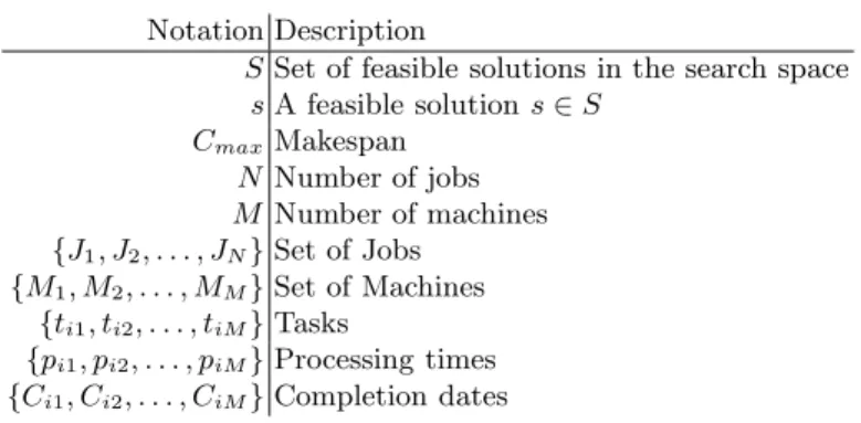
Figure 2 shows the average neutral degree to the size of the neighborhood (N −1)2_{, collected along the 30 neutral walks. Whatever the number of machines,}

the neutral degree ratio increases when the number of jobs increases. This ratio is higher for small number of machines. For 5-machine, and for 100- or 200-job and 10-machine instances, the neutral degree is huge, higher than 20%. For 100-or 200-job and 20-machine instances, the ratio seems to be very low (3.9%), but the number of neighbors with same fitness value is significant (about 382 and 1544 neutral neighbors for 100 and 200 jobs, respectively). There is no local optimum without a neighbor with the same fitness value, which means that each local optimum belongs to a local optima neutral network. The neutral degree is high enough to describe the fitness landscape with neutral networks.

A neutral walk corresponds to a sequence of neighbor solutions on a NN of the fitness landscape, where all solutions share the same fitness value. During

0 0.1 0.2 0.3 0.4 0.5 0.6 0 50 100 150 200 250

Neutral deg / Neigh. size

Number of Jobs

5 Machines 10 Machines 20 Machines

Fig. 2.Average of the neutral degree to the neighborhood size according to the number of jobs.

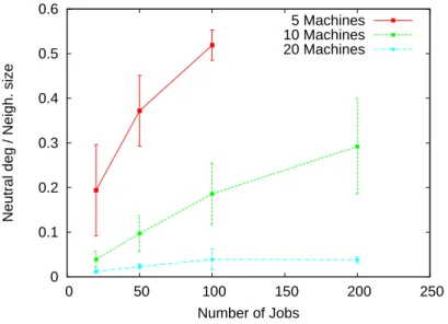
those neutral walks, we compute the autocorrelation of the neutral degree (see Section 2.3). Figure 3 shows the first autocorrelation coefficient for 5, 10 and 20 machines with respect to the number of jobs. In order to prove that those correlations are significative, we compare them to a null model. It consists of shuffling the same values of neutral degrees collected during the neutral walks. Then, the autocorrelation of this model is compared to the original one. For all sizes, the first autocorrelation coefficient of the null model is below 0.01. Therefore, we can conclude that the autocorrelation is a consequence of the succession of solutions encountered during the walk.

Obviously, for 50, 100 and 200 jobs, the neutral degree is highly correlated (higher than 0.7). Moreover, the standard deviations are very low, which indi-cates that the average values reflect properly this property on instances of same size. For 20-job and 5- or 10-machine instances, the standard deviation gets higher. This can possibly be explained by a higher correlation.

Nevertheless, these values allow us to conclude that the neutral degree of a solution is partially linked to the one of its neighbor solutions. Let us remark that the correlation for 20-job 20-machine instances is very low, due to the small average value of the neutral degree for this size.

The first conclusions of this analysis is that (i) there exists a high neutrality over the fitness landscape, particularly for large-size instances (ii) the neutral networks, defined as the graphs of neighbor solutions with the same fitness value, are not random. As a consequence, we should not expect to explore the neutral networks efficiently with a random walk. Hence, heuristic methods should exploit the information available in the neighborhood of the solutions.

0 0.2 0.4 0.6 0.8 1 0 50 100 150 200 250 ρ (1) Number of Jobs 5 Machines 10 Machines 20 Machines

Fig. 3. First autocorrelation coefficient ρ(1) computed between si and si+1 of the

neutral degree according to the number of jobs.

T1

T2

T3

?

Fig. 4.Typology of neutral networks (minimization problem).

3.3 Typology of Neutral Networks

A metaheuristic such as ILS visits several local optima. In the previous section, we have seen that the local optima often belong to a NN. A natural question arises when the metaheuristic reaches a NN: Is it possible to escape from this NN? In this section, we classify the local optima NN in three different types, and we analyze their size.

Three types of NN typologies may exist (see Figure 4):

1. The local optimum is the single solution on the NN (type T1), i.e. it has no neighbor with the same fitness value, we call it a degenerated NN.

2. The neutral walk from the local optimum did not show any neighbors with a better fitness values for all the solutions encountered along the neutral walk (type T2). Of course, as the whole NN has not been enumerated, we can not decide if it is possible to escape from them.

0 0.2 0.4 0.6 0.8 1 0 50 100 150 200 250 frequency Number of Jobs 5 Machines 10 Machines 20 Machines

Fig. 5. Average frequency of the number of degenerated neutral networks with a single solution (type T1) according to the number of jobs. 0 0.2 0.4 0.6 0.8 1 0 50 100 150 200 250 frequency Number of Jobs 5 Machines 10 Machines 20 Machines

Fig. 6. Average frequency of the number of neutral networks where no portal was found (type T2) ac-cording to the number of jobs.

0 0.2 0.4 0.6 0.8 1 0 50 100 150 200 250 frequency Number of Jobs 5 Machines 10 Machines 20 Machines

Fig. 7. Average frequency of the number of neutral networks where at least one portal was found (type T3) according to the number of jobs. -5 0 5 10 15 20 25 30 0 50 100 150 200 250 % Number of Jobs 5 Machines 10 Machines 20 Machines

Fig. 8. Average percentage of so-lutions visited at least twice along the neutral walk according to the number of jobs.

3. At least one solution having a neighbor with better fitness value than the local optimum fitness is found along the neutral walk (type T3).

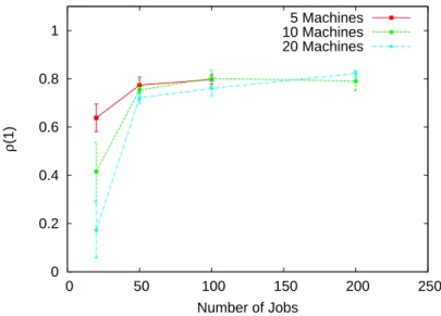
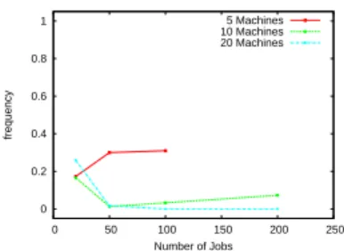
Figures 5, 6 and 7 show the proportion of NN of each type (T1, T2 or T3) counted along the neutral walks. For 50-, 100- and 200-job instances, the neutral walks show only NN of types T2 and T3. No local optimum solution is alone on the NN. For 20-job instances, the number of type (T1) is also small, except for 20 machines (25% of type T1). Hence, the neutrality is important to keep in mind while solving such instances. The number of NN without any escaping solutions found (T2) is significative only for 5-machine instances (higher than 18%) and stays very low for 10- an 20-machine instances (lower than 6%). The 20-machine instances, which are known to be the hardest to solve optimally, are the ones where the probability to escape from local optimum by neutral exploration of the NN is close to one.

When the neutral networks size is very small, the number of visited solutions is very small. Indeed, a NN of type T2 or T3 could contain very few solutions and, the neutral walk could loop on some solutions. These situations have to be considered with attention. Figure 8 shows the average percentage of solutions

-10 0 10 20 30 40 50 60 70 80 0 50 100 150 200 250 Number of Steps Number of Jobs 5 Machines 10 Machines 20 Machines

Fig. 9.Number of steps along the neutral random walk to reach the first portal ac-cording to number of jobs.

visited more than once during the neutral walk. For the 50-, 100- and 200-job instances, there is no re-visited solutions during the neutral walks. For 20-job and 20-machine instances, the number of re-visited solutions is approximatively 20% during neutral walks on NN of type T2 or T3. This result points out two remarks. First, the NN of local optima seems to be large for most instances. Second, the number of re-visited solutions is low, which means that the probability to escape the NN of type T2 is below the inverse of the size of the neutral walk.

In conclusion, for most instances, a metaheuristic could escape the local op-timum by exploring the NN. The next section will show some hints on how to guide a metaheuristic on neutral networks.

4

Exploiting Neutrality to Solve the FSP

In the previous section, we proposed to use neutral exploration to escape from local optimum, as there exists solutions having neighbor(s) with a better fitness value around neutral networks. We called those solutions, portals. An efficient metaheuristic has to find such portal with a minimum number of evaluations. First, we study the number of steps to reach a portal, and then we propose an insight to get information to find them quickly.

4.1 Reaching Portals

As shown on Figure 7 at least 70% of neutral random walks for FSP with 50, 100 and 200 jobs can reach a portal (more than 90% for 10 and 20 machines). The

performance of a metaheuristic which explores neutral networks highly depends on the probability to find a portal. Indeed, it could become more time consuming to consider a neutral walk than applying a smart restart.

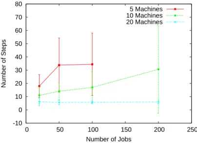
Figure 9 gives the average number of steps to reach the first portal during the 30 neutral walks. The larger the number of machines, the less the number of steps is required by the neutral walk to reach a portal. For 20-machine instances, the neutral random walks need around 7 steps to reach a portal, which is very small compared to the length of the descents (19, 40, 64, 101 respectively for 20, 50, 100, and 200 jobs). For 5-machine instances, the length of the neutral walks is around the length of the descents. Hence, it is probably more advantageous to perform a neutral random exploration than a random restart. Moreover, the fitness value obtained after the neutral walk is better than after the descent. Consequently, if an a priori study highlights that a portal is supposed to be encountered quickly, a metaheuristic that takes into account information on the neutral walk should move on the NN, and then finally find an improving solution. 4.2 How to Guide the Search?

In the previous section, the role of neutrality was demonstrated by the correlation of the neutral degree between the neutral walk neighbors and the high frequency of neutral networks. Neutral networks lead, with very few steps, to a portal. The neutrality could give interesting information about the landscape in order to guide the search. However, since the neutral network is large, the search has to be guided to find quickly a portal and not to stagnate on the NN. Thus, proper information has to be collected and interpreted along the neutral walk to help the metaheuristic to take good decision: Is it more interesting to continue the neutral walk until a portal is reached or to restart? As suggested in Section 2.3, we compute the evolvability of a solution as the average fitness values of its neighbors for all visited solutions. We analyze the evolvability of solutions on neutral networks and we give some results about the correlation of evolvability and portals on a neutral network. This allows us to propose new ideas for the design of a metaheuristic.

During those neutral walks, we compute the evolvability of each solution along the neutral walk, and then its autocorrelation (see section 2.3). Figure 10 shows the first autocorrelation coefficient ρ(1) for 5, 10 and 20 machines with respect to the number of jobs. In order to show that those correlations are significative, as in section 3.2, we compare them to a null model. For all sizes, the first autocorrelation coefficient of the null model is below 0.01. Therefore, we can conclude that the autocorrelation is a consequence of the succession of solutions encountered during the walk. The average fitness values of the neighbors are not distributed randomly: they can then be exploited by a metaheuristic.

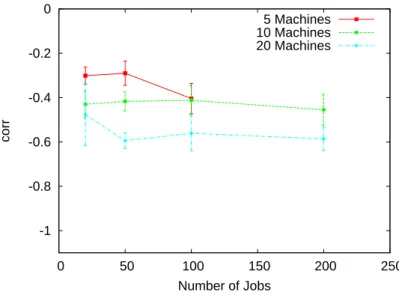
The neutral networks present evolvability and portals. So, we can wonder if the evolvability would be able to guide a metaheuristic quickly to a portal. To test this hypothesis, along the neutral walks, we compute the correlation between the average fitness values in the neighborhood and the number of steps required to reach the closer portal of the walk. This is presented in Figure 11. The larger

0 0.2 0.4 0.6 0.8 1 0 50 100 150 200 250 ρ (1) Number of Jobs 5 Machines 10 Machines 20 Machines

Fig. 10.First autocorrelation coefficient ρ(1) of the average fitness values of neighbors solutions between siand si+1according to the number of jobs.

the number of machines, the higher (in absolute value) the negative correlation. For 10- or 20-machine instances, this correlation belongs to [−0.6; −0.4], so that it is significant for a metaheuristic to use such an information. The lower the average fitness values in the neighborhood, the closer a portal is. Consequently, we propose to design a metaheuristic that takes into account the neutrality by allowing the exploration of solutions along the neutral walk. Starting from a local optimum, it would choose the next neutral solution with the lower average fitness values of its neighbors. This would increase the probability to find a portal quickly, and then to continue the search process.

5

Discussion

In this work, we studied the neutrality of the FSP on a set of benchmark in-stances originally proposed by Taillard. Most of the inin-stances have a high neutral degree: for a solution, the number of its neighbors with the same fitness value is significant in comparison to the neighborhood size. Starting from local op-tima, neutral walks have been performed. Each walk moves from a solution to another with the same fitness value and defines a neutral network that is shown to be structured. Indeed, the graph of neighbor solutions is not random and so a solution shares information with its neighbors. We show that a neutral walk leads easily to portals, solutions of the neutral network having a neighbor with a better fitness value. Furthermore, the evolvability, defined in this study as the average fitness values of the neighbors, is highly autocorrelated. It proves that this information is not random between the neighbor solutions and so it could

-1 -0.8 -0.6 -0.4 -0.2 0 0 50 100 150 200 250 corr Number of Jobs 5 Machines 10 Machines 20 Machines

Fig. 11.Correlation between the average fitness values of the neighbors and the number of steps required to reach the closer portal according to the number of jobs.

be helpful to take it into account. Besides, improving the evolvability during the neutral walk often leads to a portal. This work completes the knowledge of FSP fitness landscape, and in particular, about its neutrality. Here, the neutrality has been shown for the FSP Taillard instances where the durations of jobs are inte-ger values from [0; 99]. This is a specific choice which could have an impact on the difficulty of instances. Future works will consider other instance generators, and study the neutrality according to the instance parameters.

This work also helps to understand some experimental results on the effi-ciency of metaheuristics. In a study of iterated local search to solve the FSP [1], St¨utzle designs several efficient ILS, called ILS-S-PFSP and compares them to local search algorithms. He writes: ”Experimentally, we found that rather small modifications [of the solution] are sufficient to yield very good performance”. In section 4.1, we show that improving solutions can be reached very quickly applying insertion operator on a neutral network. So, St¨utzle’s remark can be explained by the neutrality and the high probability on the neutral networks to move on a solution with an improving neighbor. Moreover, this works sup-ports the experimentations on ILS design for 20-machine instances. The study of neutral walks highlights features that explain the efficient design of the ILS-S-PFSP. Indeed, remember that the ILS-S-PFSP, initialized with a random so-lution, applies a local search based on insertion-neighborhood mapping to get a local optimum, and then applies iteratively the steps (i) perturbation, (ii) local search, and (iii) acceptance criterion, until a termination condition is met. All acceptance criteria tested in ILS-S-PFSP are based on the Metropolis condition: they always accept a solution with equal fitness value. So the neutral moves

are always accepted. Besides, St¨utzle work shows that the perturbation based on the application of several swap operators (also called transpose operators) is efficient. And, the swap neighborhood is included in the insertion neighborhood as the job i can be inserted at the positions (i − 1) or (i + 1). So, applying the swap operator several times could correspond to a walk on a neutral network defined by insertion-neighborhood relation. Thus, steps (i) and (iii) allow the ILS-S-PFSP to move on the neutral network that could be frequent for those FSP instances. Moreover, we show that the distance is small between a local optimum and a portal. So, such an ILS-S-PFSP is able to quickly improve the current best solution, which could explain its performances.

Furthermore, our work proposes to consider the neutrality to guide a meta-heuristic on the search space. The FSP instances shows neutrality, it is easy to encounter portals along a neutral walk and the evolvability leads quickly to them. With such information, a metaheuristic is proposed: first a local search is performed from a random solution, and then iteratively (i) the evolvability on the neutral network is optimized until a portal is found and (ii) the local search is applied to move to an other local optimum. The metaheuristic finishes when the termination criterion is met. Similar ideas have been ever tested on other problems with neutrality such as Max-SAT and NK-landscapes with neutral-ity [17]. A first attempt for developing such a strategy leads to the proposition of NILS [18] that has been successfully tested on flowshop problems.

References

1. St¨utzle, T.: Applying iterated local search to the permutation flow shop problem. Technical Report AIDA-98-04, FG Intellektik, TU Darmstadt (1998)

2. Ruiz, R., Maroto, C.: A comprehensive review and evaluation of permutation flowshop heuristics. European Journal of Operational Research 165(2) (2005) 479–494

3. Ruiz, R., St¨utzle, T.: A simple and effective iterated greedy algorithm for the per-mutation flowshop scheduling problem. European Journal of Operational Research 177(3) (2007) 2033–2049

4. Nawaz, M., Enscore, E., Ham, I.: A heuristic algorithm for the m-machine, n-job flow-shop sequencing problem. Omega 11(1) (1983) 91–95

5. Graham, R.L., Lawler, E.L., Lenstra, J.K., Rinnooy Kan, A.H.G.: Optimization and approximation in deterministic sequencing and scheduling: A survey. Annals of Discrete Mathematics 5 (1979) 287–326

6. Johnson, S.M.: Optimal two- and three-stage production schedules with setup times included. Naval Research Logistics Quarterly 1 (1954) 61–68

7. Lenstra, J.K., Rinnooy Kan, A.H.G., Brucker, P.: Complexity of machine schedul-ing problems. Annals of Discrete Mathematics 1 (1977) 343–362

8. Taillard, E.: Benchmarks for basic scheduling problems. European Journal of Operational Research 64 (1993) 278–285

9. Wright, S.: The roles of mutation, inbreeding, crossbreeding and selection in evolu-tion. In Jones, D., ed.: Proceedings of the Sixth International Congress on Genetics. Volume 1. (1932)

10. Van Nimwegen, E., Crutchfield, J., Huynen, M.: Neutral evolution of mutational robustness. In: Proc. Nat. Acad. Sci. USA 96. (1999) 9716–9720

11. Wilke, C.O.: Adaptative evolution on neutral networks. Bull. Math. Biol 63 (2001) 715–730

12. V´erel, S., Collard, P., Tomassini, M., Vanneschi, L.: Fitness landscape of the cellular automata majority problem: view from the “Olympus”. Theor. Comp. Sci. 378(2007) 54–77

13. Bastolla, U., Porto, M., Roman, H.E., Vendruscolo, M.: Statiscal properties of neutral evolution. Journal Molecular Evolution 57(S) (August 2003) 103–119 14. Weinberger, E.D.: Correlated and uncorrelatated fitness landscapes and how to

tell the difference. In: Biological Cybernetics. (1990) 63:325–336

15. Altenberg, L.: The evolution of evolvability in genetic programming. In Kinnear, Jr., K.E., ed.: Advances in Genetic Programming. MIT Press (1994) 47–74 16. Verel, S., Collard, P., Clergue, M.: Measuring the Evolvability Landscape to study

Neutrality. In Keijzer, M., et al., eds.: Poster at Genetic and Evolutionary Com-putation – GECCO-2006 Genetic and Evolutionary ComCom-putation – GECCO-2006, Seattle, WA United States, ACM Press (07 2006) 613–614 tea team.

17. Verel, S., Collard, P., Clergue, M.: Scuba Search : when selection meets innovation. In: Evolutionary Computation, 2004. CEC2004 Evolutionary Computation, 2004. CEC2004, Portland (Oregon) United States, IEEE Press (06 2004) 924 – 931 18. Marmion, M.E., Dhaenens, C., Jourdan, L., Liefooghe, A., Verel, S.: NILS: a

neutrality-based iterated local search and its application to flowshop scheduling. In: 11th European Conference on Evolutionary Computation in Combinatorial Optimisation(EvoCOP11). LNCS, Springer-Verlag (2011)