The cost of equity capital for REITs : an examination of three asset-pricing models

(1)

MIT Center for Real Estate September, 2000

The Cost of Equity Capital for REITs: An Examination of Three Asset-Pricing Models

David N. Connors

Matthew L. Jackman Thesis, 2000

© Massachusetts Institute of Technology, 2000. This paper, in whole or in part, may not be cited, reproduced, or used in any other way without the written permission of the authors. Comments are welcome and should be directed to the attention of the authors.

MIT Center for Real Estate, 77 Massachusetts Avenue, Building W31-310, Cambridge, MA, 02139-4307 (617-253-4373).

(2)

THE COST OF EQUITY CAPITAL FOR REITS:

AN EXAMINATION OF THREE ASSET-PRICING MODELS

by

David Neil Connors B.S. Finance, 1991

Bentley College

and

Matthew Laurence Jackman B.S.B.A. Finance, 1996

University of North Carolina at Charlotte

Submitted to the Department of Urban Studies and Planning in partial fulfillment of the requirements for the degree of

MASTER OF SCIENCE IN REAL ESTATE DEVELOPMENT at the

MASSACHUSETTS INSTITUTE OF TECHNOLOGY September 2000

and to distribute publicly paper and electronic (\aopies of this thesis in whole or in part.

Signature of Author:

- T L- . v

Department of Urban Studies and Planning August 1, 2000

IN

Department of Urban Studies and Planning August 1, 2000 Certified by:

Blake Eagle Chairman, MIT Center for Real Estate Thesis Supervisor

Certified by: /

Jonathan Lewellen Professor of Finance, Sloan School of Management Thesis Supervisor

Accepted by:

William C. Wheaton Chairman, Interdepartmental Degree Program in Real Estate Development

(3)

THE COST OF EQUITY CAPITAL FOR REITS:

AN EXAMINATION OF THREE ASSET-PRICING MODELS by

David Neil Connors and

Matthew Laurence Jackman

Submitted to the Department of Urban Studies and Planning on August 1, 2000 in partial fulfillment of the requirements for the Degree of Master of Science in Real Estate Development

ABSTRACT

The purpose of this study is to determine a reliable asset-pricing model that can be used in practice to estimate the cost of equity capital for Real Estate Investment Trusts (REITs). While the cost of equity is an important concept for all industries, it has particular relevance for REITs, as the current environment has forced many REITs to explore new methods of increasing earnings. Hence, it is vital that REITs have an accurate benchmark on which to base new investment and capital budgeting decisions.

The first research model employed is the traditional Capital Asset Pricing Model (CAPM). In the CAPM, the total excess returns for each REIT in the sample are regressed against the total excess returns of the broad market index. The second research model incorporates the two firm-specific factors developed by Fama and French, SMB (small minus big) and HML (high minus low). In the third model, two additional macroeconomic factors are included to represent the change in expected inflation and the change in risk premium. Using factors that are of a pervasive macroeconimic nature is in line with the Arbitrage Pricing Theory of Ross.

The results indicate that the Fama-French model (FFM) is superior to the other two models in predicting excess total returns (cost of equity) for the research sample of equity REITs. This conclusion is based upon a nonparametric test comparing the fitted coefficients of determination

(R2's) from each of the regressions. Furthermore, the range of cost of equity estimates produced

by the FFM seems rational given the specific characteristics of equity REITs.

Thesis Supervisors: Blake Eagle

Chairman, MIT Center for Real Estate

Jonathan Lewellen

(4)

CHAPTER ONE

Introduction

When creditors and owners invest capital in a company, they incur an opportunity cost equal to the return that could have been earned on an alternative investment of similar risk. This opportunity cost is known as the firm's cost of capital. A company's cost of capital is often referred to as its "hurdle rate" when used to evaluate a commitment of capital to an investment or project, as it is the minimum rate of return the company can earn on existing assets and still meet the expectations of its capital providers. Depending on the level of risk for a given prospective investment relative to the company's overall risk profile, the actual discount rate may be at, above, or below the company's overall cost of capital.

The term capital in the context of a company's cost of capital refers to the components of the entity's capital structure, including long-term debt, preferred equity, and common equity. Depending on the complexity of the capital structure, a company may have additional subcategories of capital, or related forms such as warrants or options. Each component of an entity's capital structure has a unique and specific cost, which depends primarily on its respective risk.

Determining the cost of debt or preferred equity for a company is relatively straightforward. When a firm issues debt or preferred stock, it promises to pay the holder of the security a specified stream of future payments. Market rates for bonds and preferred stock of a

similar maturity and risk level can be easily identified in the marketplace. Knowing the

promised payments and the current market price of a security, it is a simple matter to calculate

(6)

Chpe n Itouto

the expected return to debt or preferred equity holders. With common equity, however, the situation becomes much more complex.

Estimating the cost of equity capital for a firm is at once the most critical and the most difficult element of most business valuations and capital expenditure decisions. The expected returns on common equity have two components: (1) dividends or distributions, and (2) changes in market value (capital gains or losses). Because these return expectations cannot be directly observed, they must be estimated from current and historical evidence. Therefore, it is necessary to look to the investment markets for the necessary data to estimate the cost of capital for any company, security, or project.

Historically, two principal approaches have been utilized to estimate a company's cost of equity capital: (1) a discounted cash flow model such as the Gordon Growth Model, and (2) a model which attempts to measure the cost of equity as a premium over some observable market rate. The first approach focuses on projections of future cash flows for a particular company and estimates the cost of equity capital as the rate that equates the current price with the present value of the cash flows. The problem with this approach is that it is very sensitive to the estimated growth rate that is employed. Furthermore, it does not incorporate systematic influences that affect capital markets and the relative returns for alternative companies (Elton, 1994). The second approach recognizes that the cost of equity should be related to a benchmark return in the capital markets, but it supplies no guidance as to what magnitude or degree a company's cost of equity should differ from a benchmark rate.

The Capital Asset Pricing Model (CAPM) was the first rigorous theoretical model used to estimate how a specific company's return should differ from an observable market rate. However, soon after it was developed researchers began to find obvious mispriced securities and

(7)

Chapter One - Introduction 6

to question the general applicability of the theory'. A fundamental criticism of the CAPM is that the pure-form equation almost always has an intercept above the riskless rate. Therefore, the model systematically understates the true cost of equity capital for any stock having a beta below one, while systematically overstating it for any stock having a beta above one (Elton, 1994).

An alternative and potentially more complete explanation of differential rates of return and the cost of equity capital was proposed by Stephen Ross in 1976 - the Arbitrage Pricing Theory (APT). In the APT model, the cost of capital for an investment varies according to that investment's sensitivity to each of several risk factors. The model itself does not specify what the risk factors are, but general applications consider only risk factors that are of a pervasive macroeconomic nature. Most academicians consider the APT model richer in its informational content and explanatory power than the CAPM.

A recent model which is gaining acceptance was developed by Eugene Fama and Ken French in the early 1990s. Fama and French propose that a security's expected return depends on the sensitivity of its return to the market and the returns on two portfolios meant to mimic these additional risk factors. The additional mimicking portfolios are SMB (small minus big) and HML (high minus low). SMB is the difference between the returns on a portfolio of small stocks and a portfolio of big stocks, measured in terms of equity capitalization. The motivation for including SMB is to capture the size premium present in historical common equity returns. The other factor, HML, is the difference between the returns on a portfolio of high-book-to-market-equity stocks and low-book-to-high-book-to-market-equity stocks. This "relative distress factor" assumes that the earnings prospects of firms are associated with a risk factor in returns.

See Chapter Four - Literature Review.

(8)

Chapter - Introduction One 7~~~~~~~~~~~~~~~~~~~~~~~~~

Irrespective of its theoretical framework, a model designed to estimate the cost of equity must be flexible and easily employable in order to be used by practitioners. A model can be theoretically sound, but if it cannot be readily applied in practice, the model will have limited value and appeal. Moreover, the model must produce results that are both accurate and stable over time. While no model will work perfectly in every instance, it should produce sensible results on a consistent basis. The main objective of this study is to develop a particular multi-factor pricing model that can be used in practice to effectively estimate the cost of equity capital for Real Estate Investment Trusts (REITs).

REITs present an interesting case study for examining the cost of equity capital. For one, the requirements and limitations of the REIT structure make the industry unique with respect to other equities. Furthermore, the relatively young industry has been continually evolving since its inception in 1960, with most of the growth occurring over the past decade. More importantly, the decline in REIT share prices and the ensuing capital crunch beginning in 1998 have caused the real estate industry to reexamine the value of the REIT structure. Hence, now more than any other time in the industry's history, it is vital that REITs have an accurate benchmark on which to base capital budgeting and investment decisions.

Existing research in real estate indicates that single factor models such as the CAPM are

not sufficient for examining the risk-return relationship or real estate-related assets2_.

Furthermore, financial literature indicates that equity REITs may possess risk-return characteristics that differ from ordinary equities. For example, real estate investments are often viewed as a hedge against the effects of inflation. Therefore, it follows that real estate portfolio returns may be the result of a multi-factor return generating function.

2 Ibid.

(9)

Chapter One - Introduction ₈

This study employs three different models to estimate the cost of equity for a defined sample of equity REITs. The first model is the traditional CAPM, with the total return on the market portfolio as the only explanatory variable in the time-series regression. This model will serve as the basis for comparison of the other two models. For the second model, the two Fama-French factors are added. In the third model, two macroeconomic variables are combined with the three existing factors, in line with Arbitrage Pricing Theory. The relative ability of the models in explaining time-series variations in equity REIT returns measured using a nonparametric test based upon the fitted coefficients of determination (R2_{'s) from each of the}

regressions.

The pages that follow will be organized around the three research models for which it is the objective of this study to explore. Prior to the presentation of the models, however, Chapter Two will present a detailed overview of REITs, including classifications, the evolution of the

modem REIT industry, and specific legal requirements. Chapter Three will provide the

theoretical background of the three models employed in this study. In Chapter Four, a literature review is presented which outlines important existing research relating to REITs and the theoretical models. Chapter Five will describe in detail each of the research models, the sample and selection criteria of the equity REITs, and the empirical results that are obtained. Finally, the results are summarized in Chapter Six, as well as some thoughts on further research on this subject.

(10)

Chapter Two - Real Estate Investment Trusts - An Overview 9

CHAPTER TWO

Real Estate Investment Trusts

-An Overview

The Real Estate Investment Trust (REIT) was formally established by the Real Estate

Investment Trust Act of 1960. Congress created the REIT vehicle to provide individual

investors with the benefits of owning and financing commercial real estate on a tax-advantaged basis. Due to the high level of both resources and knowledge that is required, few individual investors are able to directly own or finance commercial real estate properties. The REIT security allows investment in real estate without the substantial long-term commitment typical of

other real estate investment alternatives. Furthermore, the fact that most REIT stocks are

publicly traded provides additional liquidity and access to information.

There exist two principal classifications of REITs: Equity REITs and Mortgage REITs. Equity REITs acquire ownership interest in real property and derive most of their income from

Figure 2.4 the rental stream produced. Alternatively, Mortgage

REIT CLASSIFICATIONS REITs purchase mortgage obligations on real % of Total Capitalization, Year-End 1999

Hybrid property and, thus, become creditors with liens

given priority over equity positions. A third

classification, Hybrid REITs, combines elements of both Equity and Mortgage REITs. As of year-end 1999, Equity REITs comprised about 91% of total REIT capitalization, Mortgage REITs about 5%, and

ce: NAREIT Hybrid REITs 4% (NAREIT, See Figure 2.4).

Mori 51

(11)

INDUSTRY DEVELOPMENT

The first REIT was actually formed in 1963. Despite a rather slow start, REITs

experienced their first significant growth during the late 1960s and early 1970s. Specifically, total REIT assets increased by nearly 2000% from 1968 to 1973 (Han and Liang, 1995). This period of expansion was attributable to the strong demand for construction and development funding which was not being satisfied by traditional capital sources. REITs were able to provide long-term capital sourced from short-term paper and bank financing. Since there existed large spreads between the rates charged for construction and development loans and short-term interest rates, many REITs enjoyed very high returns during this period.

Continued demand for capital allowed mortgage REITs to enjoy high profits until interest rates began to rise in 1972 and 1973. The previously high spreads began to disappear, and

eventually became negative, forcing many REITs to operate at a net loss. Furthermore,

overbuilding in the real estate industry forced many developers to default on their existing loans. REIT valuation was severely affected, and the NAREIT Index dropped by over 56% from January 1973 to January 1975 (NAREIT).

The REIT industry witnessed several significant structural changes in the late 1970s and early 1980s. Due to the negative experiences of the previous recession, REIT leverage was greatly reduced. Average leverage ratios declined from 64% in 1972 to 55% by 1984. Short-term debt also declined from 44% of total assets in 1972 to 8% in 1984. Furthermore, construction and development loans as a percent of total REIT assets declined from 53% to 6%

over the same time period (Han and Liang, 1995).

A major impact on the growth of REITs was the passing of the Tax Reform Act (TRA) of 1986. The TRA eliminated the tax advantages of real estate limited partnerships by lengthening

(12)

depreciation schedules and replacing accelerated depreciation with the straight-line method. Furthermore, the new law no longer allowed non-cash losses from passive investments (such as real estate) to shelter ordinary income. These changes made investment in REITs comparatively attractive to direct ownership of real estate.

The REIT industry believed that the tax law changes would allow REITs to play a much more significant role in real estate investment. In preparation, the industry, led by the National Association of Real Estate Investment Trusts (NAREIT) and a dedicated group of REITs and associated law and accounting firms, convinced Congress to include a package of REIT "modernization" amendments to the 1986 tax reform legislation. These proposals allowed for important changes such as REIT subsidiaries, expansion of the prohibited transaction safe harbor for REITs that needed to sell or dispose of properties, and greater flexibility by REIT

management to make short-term investments of newly raised capital. Of these 13 new

amendments, none was more important than the alteration of the independent contractor requirement, permitting REITs to perform property management services that were "usual and customary" for their tenants (Garrigan, 1998).

Improvements in the external environment coupled with much-needed capital structure

revisions allowed REITs to slowly recover from the crisis in the mid-1970s. Most of this

recovery occurred in the late 1980s through the mid-1990s, as the modern REIT industry began to take shape.

(13)

THE MODERN REIT INDUSTRY

The real estate industry witnessed a severe recession in the late 1980s and early 1990s. As a result, traditional capital suppliers such as banks, savings and loan institutions, and life insurance companies all exited the real estate capital markets in the face of weak demand and massive over-building. The liquidity crisis led to a dramatic reduction in value of existing

properties, and provided an opportunity for the REIT industry to expand. Healthy,

low-leveraged balance sheets and unparalleled access to inexpensive equity capital enabled REITs to replace previous capital sources, which led to a period of record growth.

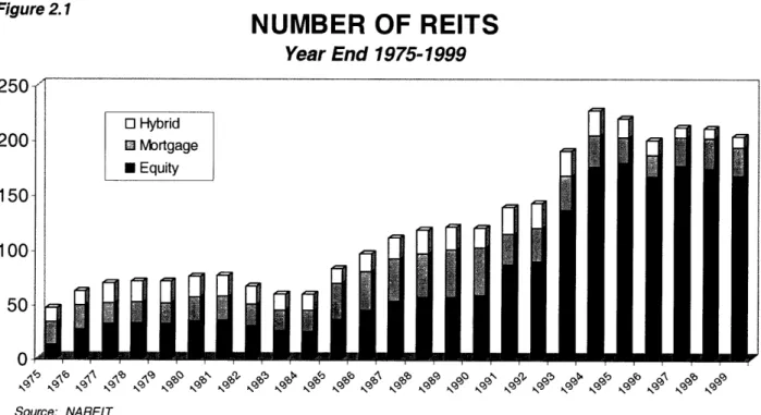
The success of the REIT structure set off an IPO frenzy in the early 1990s. Nearly two-thirds of all publicly traded equity REITs in existence today have been formed since 1990. In 1993 and 1994 alone, 95 companies went public raising over $16.5 billion in equity (NAREIT). The total number of REITs increased from 119 at the beginning of the decade to a high of 226 by year-end 1994 (see Figure 2.1). Total market capitalization in nominal terms went from $8.74

Figure 2.1

NUMBER OF REITS

Year End 1975-1999 e3V -200 150- 100- 50- n-,orny 'A9llllil1lll l [ _ __ _ _ __ '9 . . . .I . . . . Source: NAREIT o Hybrid 0 Mortgage * Equity

nj?

8

lUiiiiN11

A

--]

I

laa -- r IC -aL cl 8·- Bll IC 481gi1 , _ . _t

v ' ' ' ' ' ' ' ' ... ' · ' · '~~~~~~~~~~~~ii · l rImI I or

(14)

billion in 1990 to a high of $140.5 billion at year-end 1997 (see Figure 2.2) 3. At year-end 1999, there were a total of 203 REITs with a total market capitalization of $118,233 million.

Figure 2.2

EQUITY MARKET CAPITALIZATION

Year End 1975-1999 $160,000 $140,000 $120,000 $100,000 * $80,000 $60,000 $40,000 $20,000 $0 Source: NAREIT

A significant event that helped pave the way for the IPO explosion was the advent of the umbrella partnership (UPREIT) structure first used in the 1992 offering of Taubman Centers. Using the UPREIT structure enabled owners of "low tax basis" properties to defer or, at best,

eliminate capital gains liabilities. The UPREIT is a structure in which a partnership is

established to hold title to the assets and liabilities of the firm. The partnership, in turn, is owned by the REIT and the existing investors in the company that is going public. The REIT itself is owned by its shareholders. An additional advantage to the UPREIT structure is the future possibility of using UPREIT equity interests as currency in tax-deferred acquisitions (Garrigan,

(15)

Chapter Two - Real Estate Investment Trusts - An Overview 14 1998). However, an important drawback of the structure is that, because of differing tax liabilities, it creates a conflict between owners of UPREIT units and common shareholders. Nevertheless, without the creation of the UPREIT structure, many of the top real estate companies could not (or would not) have chosen to go public. Of the 100 largest REITs, 52 are organized using the UPREIT format (NAREIT).

The ability of REITs to take advantage of deflated property prices resulted in high returns for shareholders. For the period 1979 through 1997, equity REITs had a total annual return of

nearly 15% versus 9% for direct property investment (NAREIT, see Table 2.3)4_{. However, by}

1998, liquidity began to return to the real estate markets and share price multiples of REITs began to increase. This resulted in higher capital costs, and many REITs found it increasingly difficult to find accretive acquisition opportunities. For the first time, many REITs became net sellers of assets. Share prices began to fall, and the sector moved from trading at greater than a 20% premium to net asset value (NAV) to trading at greater than a 20% discount (Riddiough, 2000). While REITs still provided an attractive dividend yield, the total annual returns for the NAREIT Index for 1998 and 1999 were -19% and -7%, respectively.

OUTLOOK

As the real estate environment began to change in the late 1990s, it became evident that the context of the 1992 to 1996 period of growth for REITs would not be the context of the future. Changes in the macroeconomic environment will test the viability of the REIT structure in new ways, as REITs are forced to produce increasingly more challenging levels of earnings growth in order to meet the expectations of Wall Street.

(16)

Chapter Two - Real Estate Investment Trusts - An Overview

Table 2.3

Investment Performance of All Publicly Traded REITs1

(Percentage changes, except where noted, as of December 31, 1999)

COMPOSITE Return Components Dividend Period Total Price Income Yield2

EQUITY

Return Components Dividend Total Price Income Yield2

MORTGAGE

Return Components Dividend Total Price Income Yield2

HYBRID

Return Components Dividend Total Price Income Yield2

1988 11.36 1.24 10.11 10.03 13.49 4.77 8.72 8.57 7.30 (5.12) 12.42 13.19 6.60 (2.87) 9.47 9.61 1989 (1.81) (12.06) 10.25 10.19 8.84 0.58 8.26 8.42 (15.90) (26.19) 10.28 13.56 (12.14) (28.36) 16.22 10.22 1990 (17.35) (28.49) 11.15 11.34 (15.35) (26.45) 11.10 10.15 (18.37) (29.18) 10.81 13.48 (28.21) (38.88) 10.67 13.18 1991 35.68 23.10 12.58 9.19 35.70 25.47 10.22 7.85 31.83 13.93 17.91 13.49 39.16 27.08 12.08 8.89 1992 12.18 2.87 9.31 7.88 14.59 6.40 8.19 7.10 1.92 (10.80) 12.72 11.21 16.59 7.21 9.38 7.36 1993 18.55 10.58 7.96 7.29 19.65 12.95 6.70 6.81 14.55 (0.40) 14.95 10.89 21.18 12.44 8.75 7.69 1994 0.81 (6.41) 7.22 8.04 3.17 (3.52) 6.69 7.67 (24.30) (33.83) 9.53 13.52 4.00 (5.95) 9.95 8.31 1995 18.31 9.12 9.19 7.49 15.27 6.56 8.71 7.37 63.42 46.80 16.62 9.02 22.99 13.10 9.89 7.70 1996 35.75 26.52 9.23 6.22 35.27 26.35 8.92 6.05 50.86 37.21 13.65 8.50 29.35 19.70 9.65 6.72 1997 18.86 11.85 7.01 5.73 20.26 13.33 6.93 5.48 3.82 (3.57) 7.40 9.41 10.75 2.79 7.96 7.35 1998 (18.82) (23.82) 5.00 7.81 (17.50) (22.33) 4.83 7.47 (29.22) (34.29) 5.07 10.49 (34.03) (42.16) 8.13 13.07 1999 (6.48) (14.06) 7.59 8.98 (4.62) (12.21) 7.59 8.70 (33.22) (40.12) 6.90 13.53 (35.90) (43.43) 7.53 17.24 ... . ... .. .... A.. .. .... .. .. .. ...'s 1998:04 (3.94) (5.49) 1.56 7.81 (2.92) (4.43) 1.51 7.47 (18.04) (19.54) 1.50 10.49 (7.21) (10.09) 2.88 13.07 1999:Q1 (5.10) (6.81) 1.71 8.03 (4.82) (6.56) 1.74 7.96 (6.47) (7.44) 0.97 8.08 (15.14) (17.38) 2.24 11.74 Q2 10.58 8.56 2.02 7.39 10.08 8.11 1.97 7.34 21.35 18.70 2.65 7.10 10.51 7.46 3.05 10.94 Q3 (9.28) (11.23) 1.95 8.39 (8.04) (10.01) 1.97 8.27 (31.91) (33.21) 1.30 9.35 (14.55) (17.15) 2.60 13.23 04 (1.76) (4.31) 2.54 8.98 (1.01) (3.44) 2.43 8.70 (13.60) (18.41) 4.81 13.53 (20.00) (23.09) 3.09 17.24 1-Year (6.48) (14.06) 7.59 (4.62) (12.21) 7.59 (33.22) (40.12) 6.90 (35.90) (43.43) 7.53 3-Year (3.37) (9.87) 6.50 (1.82) (8.24) 6.41 (21.12) (27.61) 6.48 (22.34) (30.45) 8.12 5-Year 7.70 0.22 7.49 8.09 0.79 7.30 3.88 (5.24) 9.12 (5.71) (14.56) 8.84 10-Year 8.10 (0.54) 8.64 9.14 1.08 8.06 1.41 (9.65) 11.06 0.90 (8.73) 9.63 15-Year 6.81 (2.17) 8.98 9.77 1.63 8.14 (0.07) (11.08) 11.01 0.30 (9.74) 10.04 20-Year 10.28 0.59 9.70 12.34 3.20 9.14 4.27 (7.25) 11.52 6.15 (4.03) 10.18 Source: NAREIT

Includes all REITs that trade on the New York Stock Exchange, American Stock Exchange and NASDAQ National Market List. Data prior to 1999 are based on published monthly returns through the end of 1998.

2 Dividend yield quoted in percent for the period end.

As mentioned earlier, REITs were able to grow earnings through purchasing properties at relatively high capitalization rates then packaging and reselling them to the public at yields that were 200 to 400 basis points lower. This practice of "positive spread investing" became increasingly more difficult as the real estate markets moved further into recovery. By 1998, heightened competition for properties drove prices up (and capitalization rates down) to the point that the large yield spreads had all but disappeared. No longer able to grow through acquisition,

(17)

REITs were forced to devise more creative strategies to increase earnings. This has led to much riskier strategies such as increased real estate development, movement into new markets, and joint venture agreement with other public and private real estate companies.

In the current environment, it is extremely important that REIT management can accurately measure and thoroughly understand the company's cost of capital. The decline in REIT share prices and the ensuing capital crunch beginning in 1998 have caused real estate investors to question the true value of the REIT structure. Hence, as REITs continue to explore new methods of increasing earnings, it is vital they have an accurate benchmark on which to base investment decisions. The goal of this study is to identify a model that can be used by REIT industry practitioners to accurately estimate the cost of equity capital.

REIT LEGAL STRUCTURE

The advantage of the REIT form of organization is that it is exempt from corporate-level taxation. It is estimated that the overall value of the REIT tax shield is about 2-5% of industry equity market capitalization, although higher for firms with lower-than-average payout ratios. (Gyourko and Sinai, 1999). There are, however, numerous conditions that must be met in order to qualify for tax-preferred status. The primary drawback of the REIT structure is the limited ability to retain earnings, an important issue given the capital-intensive nature of real estate.

The conditions for REITs are contained in Sections 856 to 860 and related sections of the Internal Revenue Code. These conditions can be subdivided into organizational, asset-related, income-related, distribution requirements, and compliance requirements. Below is a summary of the qualifying factors.

(18)

Organizational Requirements

The entity must file an election form to be taxed as a Real Estate Investment Trust with its annual tax return. A REIT must be a corporation, trust, or association with transferable shares and be taxable as a domestic corporation. It may not be a financial institution or insurance company. The REIT must have at least 100 or more persons that own its stock or beneficial interests. Furthermore, no more than 50% of the total outstanding shares may be held either directly or indirectly by any group of five or fewer individuals during the last half of the REIT's

taxable year. For this purpose, corporations, partnerships, and pension funds are "looked

through" to their ultimate individual shareholders or beneficiaries.

Asset Requirements

At least 75% of the value of the REITs assets must consist of real estate, cash, or Government Securities. Not more than 25% of total asset value may consist of securities, other than those included in the 75% test. The REIT may not have more than 5% of its assets invested in the securities of one issuer. Moreover, a REIT may not hold more than 10% of the outstanding voting non-real estate shares of any one issuer.

Income Requirements

At least 75% of a REITs gross income must be derived from rents from real property or interest on mortgages secured by real property, gains from the sale of real property not held for sale in the ordinary course of business, dividends from qualified REITs, gain from sale or qualified REIT stock, refund of taxes on real property, or gain from sale of foreclosed property.

(19)

At least 95% of a REIT's gross income must come from sources that satisfy the 75% test, dividends, interest, or gain from the sale of stocks or securities. In addition, not more than 30% of the REIT's income can be derived from the sale or disposition of stock or securities held less than six months, or real property held less than four years (other than property involuntarily converted or foreclosed upon).

Distribution Requirements

Currently, at least 95% of a REIT's taxable income (excluding net capital gains) must be distributed to shareholders in the form of dividends. However, pursuant to the 1999 REIT Modernization Act, this requirement will return to the 90% level that applied to REITs from

1960 through 1980 beginning in 2001.

Compliance Requirements

Shareholders of the REIT must be polled annually to determine ownership of the outstanding shares and to ascertain whether or not the REIT has fulfilled the requirements of the "five or fewer" ownership rule. In addition, the quarterly "asset" and "income" tests must be supported by sufficient accounting records.

(20)

Chapter Three - The Theoretical Models 19

CHAPTER THREE

The Theoretical Models

THE CAPITAL ASSET PRICING MODEL

The Capital Asset Pricing Model (CAPM) was developed by William Sharpe in 19645. The CAPM is part of a larger body of economic theory known as Capital Market Theory (CMT). CMT also includes security analysis and portfolio management theory, a normative theory that describes how investors should behave in selecting stocks for individual portfolios. The CAPM, however, is a positive theory as it describes the market relationships that will result if investors behave in the manner prescribed by portfolio theory (Pratt, 1998).

Capital market theory divides total risk into two components, systematic risk and

unsystematic risk. Systematic risk represents the uncertainty of future returns due to the

sensitivity of a particular investment to movements in the returns of the market portfolio. Alternatively, unsystematic risk is a function of the particular characteristics of an individual company, a specific industry, or the type of investment interest. The total risk of an investment depends on both systematic and unsystematic risk factors. However, capital market theory makes the assumption that investors can diversify away unsystematic risk by holding stocks in large, well-diversified portfolios. Therefore, in the CAPM, the only risk that affects the expected return on a stock (and hence the cost of equity capital) is systematic risk.

5 See Sharpe, W.F. "Capital Asset Prices: A Theory of Market Equilibrium Under Conditions of Risk." Journal of

Finance, (1964) 19, 425-42.

(21)

Chapter Three - The Theoretical Models 20

The CAPM leads to the conclusion that the equity risk premium (the required excess return for a security above the risk-free rate) is a linear function of the security's beta coefficient. This function is described in the following equation:

KEi = f + Bi [E(Rm) - Rf ] where: KEi Rf Bi E(Rm) (1)

= Cost of equity (expected return) for firm i = Risk free rate of interest

= The sensitivity of stock i return to the market return = Expected return on the market

This relationship can be seen graphically in Figure 3.1 below:

Figure 3.1 Expected Rate of Return ity t Line 1.0 Beta

The above figure shows that the beta for the market as a whole is 1.0. Therefore, from a numerical standpoint, the factor beta has the following interpretations:

(22)

Chapter Three - The Theoretical Models 21 Beta > 1.0 The rates of return for the subject company tend to move in the same direction and with greater magnitude than the market returns. Many high tech companies are examples of stocks with high betas.

Beta = 1.0 Movements in the rates of return for the subject tend to equal movements in the rates of return for the market portfolio.

Beta < 1.0 When the market rates of return fluctuate, rates of return for the subject company tend to also fluctuate, but to a lesser extent. Examples of low beta stocks include equity REITs and utilities.

Beta < 0 Rates of return for the subject company tend to move in the opposite direction from changes in the market portfolio. Stocks with negative betas are very rare.

The CAPM, like most economic models, offers a theoretical framework for how relationships should exist if certain assumptions hold. It is imperative that anyone who chooses to employ the CAPM to predict returns or estimate the cost of equity understands the assumptions underlying the model. The extent to which these assumptions are or are not met in a real world application will have an impact on the usefulness of the CAPM for the valuation of projects or investments. The main assumptions are listed below.

1. Investors are risk averse.

2. Rational investors seek to hold fully efficient (fully diversified) portfolios. 3. All investors have identical investment time horizons.

4. All investors have identical expectations about such variables as expected rates of return and how capitalization rates are generated.

5. There exist no transaction costs.

6. There are no investment-related taxes

7. The borrowing and lending rates are equivalent. 8. The market has perfect divisibility and liquidity.

(23)

Since its inception, the simple yet powerful linear prediction of the CAPM has been the subject of a large body of empirical research, and a number of studies have been published which provide both theoretical and empirical criticisms of the model6_{. These studies show that stock} returns may be related more to firm-specific variables such as size, price-to-earnings ratio, book-to-market equity ratio, and the leverage ratio. Recently, Fama and French (1992) found that the CAPM beta fails to describe average stock returns over the past fifty years if just two firm-specific variables are introduced: size and book-to-market equity.

A fundamental criticism of the CAPM is that the pure-form equation almost always has an intercept above the riskless rate. Therefore, the model systematically understates the true cost of equity capital for any stock having a beta below one, while systematically overstating it for any stock having a beta above one (Elton, 1994). Since real estate as an asset class tends to have a beta less than one, the CAPM is not a useful indicator of the true cost of equity for real estate companies. In a recent study, Chen, Hsieh, Vines, and Chiou (1998) determine that the insignificance of the market beta in their analysis leads to the rejection of the CAPM for equity REITs7.

Despite criticisms, financial theorists and practitioners alike have generally held that using the CAPM is the preferred method to estimate the cost of equity capital. Its relevance to business valuations and capital budgeting is that businesses, business interests, and business investments are a subset of the investment opportunities available in the total capital market. Hence, the determination of the prices of businesses, theoretically, should be subject to the same

6 See Brennan (1970 & 1971), Black (1972), Roll (1977), Breeden (1977 & 1989), Basu (1977 & 1983), Banz (1981), Reinganum (1981), Keim (1983), Brown (1983), Rosenburg et al. (1985), Chen et al. (1988), Bhandari (1988).

(24)

economic forces and relationships that determine the prices of alternative investment assets (Pratt, 1998).

THE FAMA-FRENCH MODEL

The Fama-French Model (FFM) is a multiple linear regression model developed by

Eugene Fama and Ken French in the early 1990s8. The FFM can be thought of as a multivariate

extension of the CAPM. The intuition is that there exist other factors that impact security prices in addition to the movement of the market and the risk free rate. Fama and French propose that a security's expected return depends on the sensitivity of its return to the market and the returns on two portfolios meant to mimic these additional risk factors (Fama and French, 1997).

The additional mimicking portfolios are SMB (small minus big) and HML (high minus low). SMB is the difference between the returns on a portfolio of small stocks and a portfolio of big stocks, measured in terms of equity capitalization. The motivation for including SMB is to capture the size premium present in historical common equity returns. Many empirical studies performed since the CAPM was originally developed indicate that the realized total returns on smaller companies have been substantially greater than predicted returns over a long period of time9.

The other factor, HML, is the difference between the returns on a portfolio of high-book-to-market-equity stocks and low-book-high-book-to-market-equity stocks. This "relative distress factor" assumes that the earnings prospects of firms are associated with a risk factor in returns. Firms that the market judges to have poor earnings prospects, signaled by low stock prices and high

8 See Fama, E.F., and K.R. French. "The Cross-Section of Expected Stock Returns." Journal of Finance (1992) 47,

427-65, and "Common Risk Factors in the Returns on Stocks and Bonds." Journal of Financial Economics (1993)

33, 3-56.

9 See Banz (1981), Huberman and Kandel (1987), Berk (1995), etc.

(25)

ratios of book-to-market equity, have higher expected stock returns (hence, a higher cost of equity capital) than firms with strong earnings prospects (Fama and French, 1992).

The expected return equation of the Fama-French Model is the following:

KE = Rf + Bil[E(Rm) - Rf ]+ Bi2[E(SMB)] + Bi3[E(HML)] (2)

where:

KEi = Cost of equity (expected return) for firm i

Rf = Risk free rate of interest (20-year T-Bond)

Bil = The sensitivity of stock i return to the market return

E(Rm) = Expected return on the market

Bi2 = The sensitivity of stock i to the return of a portfolio that mimics SMB

E(SMB) = Expected return on a portfolio that mimics SMB

Bi3 = The sensitivity of stock i to the return of a portfolio that mimics HML

E(HML) = Expected return on a portfolio that mimics HML

Fama and French use six value-weighted portfolios formed on size and book-to-market equity to construct the two specific risk factors in their model. Each year, all NYSE stocks on the Center for Research in Securities Pricing (CRSP) tapes are ranked based upon price times number of shares. The median NYSE size is then used to split NYSE, AMEX and NASDAQ stocks into two groups, small (S) and big (B). In addition, they also divide the stocks into three book-to-market equity groups based upon the bottom 30% (Low), middle 40% (Medium), and top 30% (High) of the ranked values.

In their analysis, Fama and French define book common equity as the COMPUSTAT book value of shareholders' equity plus balance-sheet deferred taxes and investment tax credit minus the book value of preferred stock. The ratio of book-to-market equity is book common equity for the fiscal year ending in calendar year t-l, divided by market equity at the end of December of t-1 (Fama and French, 1993). It is interesting to note that only firms with ordinary

(26)

common equity (as classified by CRSP) are included in the tests. This means that ADRs, REITs, and units of beneficial interest are excluded.

Fama and French then construct the six portfolios from the intersections of the two size and three book-to-market equity groups. Monthly value-weighted returns on the six portfolios are calculated from July of year t to June of t+l, and the portfolios are reformed in June of t+l. The portfolio SMB is the difference each month between the simple average of the returns on three small-stock portfolios (S/L, S/M, and S/H) and the simple average of the returns on the three big stock portfolios (B/L, B/M, and B/H). Thus, SMB is the difference between the returns on small-and big-stock portfolios with about the same weighted-average book-to-market equity. This ensures the difference will be largely free of the influence of the book-to-market equity factor, focusing instead on the different return behaviors of small and big stocks (Fama and French, 1993).

The portfolio HML is defined in the same manner as SMB. HML is the difference each month between the simple average of the returns on the two high book-to-market equity portfolios (S/H and B/H) and the average of the returns on the two low book-to-market equity portfolios (S/L and B/L). The two components of HML are returns on high and low book-to-market equity portfolios with about the same weighted-average size. As a result, the difference between the two returns should be largely free of the size factor in returns. Evidence of the success of this simple procedure is reflected in the extremely low correlation between the two monthly mimicking returns (Fama and French, 1993).

The results of Fama and French's initial study (1992) indicate that the CAPM beta does not help explain the average returns on NYSE, AMEX, and NASDAQ stocks for the period 1963

(27)

significant predictors of returns over the same period. Similar results were obtained in

subsequent studies by Fama and French, as well as other researchers. The lack of support for the CAPM is not surprising, as much of the financial research completed in the past 15 years arrives at the same conclusion. However, the work of Fama and French is significant in that it shows how two easily-measured variables can be used in practice to predict the cost of equity capital.

THE ARBITRAGE PRICING MODEL

The concept of Arbitrage Pricing Theory (APT) was introduced by Stephen Ross in 19761°. Similar to the FFM, APT can also be thought of as a multivariate extension of the CAPM. In the APT model, the expected return (cost of equity) for an investment varies according to that investment's sensitivity to a variety of risk factors, one of which may be a CAPM-type market risk. The model itself does not specify what the risk factors are, but most applications consider risk factors that are of a pervasive macroeconomic nature. Examples of common risk factors used include unanticipated inflation, the unanticipated change in the term structure, the unanticipated change in risk premium, and the unanticipated change in the growth rate in industrial production.

In APT, as in the CAPM, there exist two sources of risk for any individual stock. First is the risk associated with the macroeconomic factors which cannot be eliminated through diversification, or systematic risk. Second is the risk arising from the possible events that are unique to the specific company, or unsystematic risk. As with the CAPM, it is assumed that this company-specific risk can be eliminated through holding stocks in large, well-diversified

(28)

portfolios. Therefore, the expected risk premium on a stock is affected only by factor or macroeconomic risk (Brealey & Myers, 2000).

The econometric estimation of the Arbitrage Pricing Model (APM) with multiple risk factors yields the following formula:

KE = Rf + Bil[E(K9)]+ Bi2[E(K2)] +... + Bin[E(Kn)] (3)

where:

KE = Cost of equity (expected return) for firm i

Rf = Risk free rate of interest (20-year T-Bond)

Bin = The sensitivity of stock i return to the return of a portfolio that mimics Kn

E(K,) = Expected return on a portfolio that mimics factor K,

Notice that the APT formula makes two important statements (Brealy & Myers, 2000): 1. If a value of zero is plugged into each of the factor betas, the expected risk premium

is zero. A diversified portfolio that is constructed to have zero sensitivity to each macroeconomic factor is essentially risk-free, and therefore must be priced to offer the risk-free rate of interest. If this did not hold, investors could make an arbitrage profit.

2. A diversified portfolio that is constructed to have exposure to a factor will offer a risk premium which will vary in direct proportion to the portfolio's sensitivity to that factor. For example, if portfolio A is twice as sensitive to a factor as portfolio B, portfolio A must offer twice the risk premium. If this did not hold, investors could make an arbitrage profit.

If the arbitrage pricing relationship as it is described above holds for all diversified portfolios, then it must generally hold for individual stocks. Each stock must offer an expected return commensurate with its contribution to portfolio risk. In the framework of APT, this contribution depends on the sensitivity of the stock's return to the unexpected variations in the

(29)

Most academicians consider the Arbitrage Pricing Model (APM) richer in its informational content and explanatory and predictive power than the CAPM. Empirical research suggests that the multivariate APM explains expected rates of returns more effectively than the

univariate CAPM11_{. In fact, some researchers (Roll and Ross, 1980) propose APT as a testable}

alternative, and perhaps natural successor to the CAPM.

1" See Chen (1983), Bower et al. (1984), Chen et al. (1986), and Berry et al. (1988).

(30)

Chapter Four - Literature Review 29

CHAPTER FOUR

Literature Review

REITs and the CAPM

Much research has been done comparing the returns of REITs to the returns of the overall stock market. Although the results of these studies vary, essentially, the findings suggest that REIT risk-adjusted returns have been superior to those of other stocks from the-mid 1960s through the early 1980s, with a small number of aberrations. However, stock market portfolios have dominated REIT returns since the mid-1980s.

One of the first studies to specifically compare the performance of equity REITs with that of common stocks was by Smith and Shulman (1976). They tracked the quarterly returns of 16 equity REITs over eleven years from 1963 to 1974. These returns were contrasted against those of the S&P composite index and a sample of closed-end funds by employing various measures

including comparing geometric mean returns, goodness of fit (R2_{), and CAPM. The findings}

revealed that equity REITs underperformed the broader market and fared about the same as the closed-end funds. However, by reducing the holding period by one year (thus eliminating 1974, a year in which the stock market experienced particularly high negative returns) equity REIT's outperformed the S&P composite index.

In a subsequent study, Burns and Epley (1982) demonstrate that adding equity REITs to a portfolio of common stocks results in a more efficient portfolio frontier. The data examines quarterly returns, which include 35 REITs (10 equity REITs) from the first quarter of 1970 through the fourth quarter of 1979. The study explores various combinations of assets in order to obtain the highest efficient portfolio frontier. Previous studies indicate that the correlation

(31)

Chapter Four - Literature Review

coefficients between real estate and stocks is assets produces a more efficient portfolio. 1970 through 1979, confirm that the outcome surpasses single-asset portfolios at all points return. Furthermore, this mixed asset portfolio period.

30

s generally rather low. Hence, combining these kccordingly, the results from the period between of combining portfolios of both REITs and stocks along the efficient frontier in terms of risk and outperformed the S&P 500 index during the same

The findings of Walther (1986) and Kuhle (1987) reveal that REIT stocks outperformed the S&P index during the 1977-1984 period, but underperformed the index from 1973-1976. These results are also supported by research by Sagalyn (1990). This study examines the ex-post real returns of REITs over the period from 1973 to 1987 and shows that equity REITS exhibited

less volatility with higher returns in comparison to the S&P 500 index.

A study by Howe and Shilling (1990) suggests that REITs have underperformed the CRSP Equally-Weighted index from 1973 to 1987. In agreement with this, Gobel and Kim

(1989) examine the returns of 32 REITs over a four-year period from 1984-1987. They

compared their findings to the S&P 500 index, the Consumer Price Index, and Treasury bills. Their results indicate that the sample of REITs underperformed the S&P 500 index over the study period.

The findings from a research study performed by Martin and Cook (1991) determine through using generalized stochastic dominance that stock portfolios generated slightly higher risk-adjusted returns for the period between 1980-1990. Han and Liang (1995) studied eight REIT portfolios during 1970-1993. Their results indicate that REIT stock performance was slightly worse than the stock market portfolio. More recently, Chen and Peiser (1999) conclude

(32)

Chapter Four - Literature Review 31

that equity REITs underperformed both the S&P 500 index and the S&P Midcap 400 index over the period 1993 through 1997.

REITs and the FFM

Up to this point, there have been no previous research projects which specifically use the Fama-French model to estimate the returns of equity REITs. However, Fama and French completed a study in 1997 which employs both the CAPM and the FFM to examine the cost of equity for 48 industries, including Real Estate, for the period 1963 through 199412. Unfortunately, the Real Estate industry used in the study did not include REITs. Fama and French used four-digit SIC codes to form their industry groups, and because REITs have their own SIC code separate from other real estate companies, they were included in a general Finance industry. The results from the study are worth noting, however, as they provide additional rationale for employing the FFM in our research.

Not surprisingly, the results from the 1997 study show large differences between the cost of equity estimates obtained using CAPM and those using the FFM. For the five-year estimates, the CAPM and FFM figures differ by more than 2% for 19 industries and by more than 3% for 15 industries (Fama and French, 1997). These differences are attributable to the SMB and HML slopes in the three-factor regressions. Those industries with slopes close to zero consequently produce results similar to the CAPM. Examples of industries where this occurs is Food, Machinery, Electrical Equipment, Boxes, Building Materials, and Insurance.

Industries for which the CAPM and FFM produced significantly lower estimate for the cost of equity include health industries (Health Services, Medical Equipment, and Drugs) and

(33)

high-tech industries (Computers, Chips, and Laboratory Equipment). This result is largely due to strong negative risk loadings on the HML factor. The FFM identifies these as industries with strong growth prospects over the sample period and rewards them with comparatively lower costs of equity.

Conversely, many industries, including Real Estate, have cost of equity estimates using the FFM that are at least 2% higher than those obtained using the CAPM. Specifically, Fama and French estimated the industry cost of equity premium for Real Estate to be 5.99% using the CAPM and 11.16% using the FFM . This dramatic difference is a function of the low beta of real estate assets and the lack of significance of the CAPM in predicting returns for real estate

companies. Other industries where similar discrepancies also observed include Textiles,

Banking, Steel, and Autos. The FFM assigns high costs of equity for each of these industries because their returns covary with the returns on small stocks (they have large positive slopes on SMB) and because they behave like distressed stocks (they have large positive slopes on HML).

REITs and APT

There have been a number of research studies done in the past which attempt to link the returns from real estate to market-level factors. Many studies indicate that certain variables such as inflation and interest rates may be significant in predicting returns to real estate'3_{. In recent} years, researchers have used Arbitrage Pricing Theory to examine macroeconomic influences using publicly traded REITs as the real estate proxy. The results from these studies vary widely depending on the sample of REITs chosen and the time period examined. However, in most

13 See Hartzell et al. (1987), Fama and Schwert (1977), Rubens et al. (1989), Brueggeman et al. (1984), Ibbotson an

(34)

Chpe or-Ltrtr eiw3

cases, multifactor models are more effective at predicting REIT returns than the single-factor CAPM.

Titman and Warga (1986)

Titman and Warga's is the first study to specifically examine the risk-adjusted performance of REITs using both the CAPM and APT. Since it was generally viewed that the returns from REITs, as well as real estate in general, were sensitive to inflation and interest rates, Titman and Warga set out to examine whether the APM provided more accurate measures of risk-adjusted returns.

The research sample consists of 16 equity and 20 mortgage REITs listed on the NYSE and AMEX in 1973. The study examines the returns over two sample periods, January 1973 through December 1977, and January 1978 through December 1982. The single index, or CAPM, models employ both the CRSP Value-Weighted index and Equally-Weighted index as the market proxy. Two types of multiple-index models are also examined. The first includes a portfolio of long-term government bonds along with the (Equally-Weighted or Value-Weighted) market portfolio in a two-factor model. In addition, a model using five-factor portfolios formed

with maximum likelihood factor analysis is also examined. In theory, these portfolios are

designed to mimic changes in inflation, interest rates, and any other macroeconomic variables that generate returns on capital assets.

The results of the study suggest that the single-index and multiple-index models can provide very different estimates of the performance of REITs. In particular, the performance measures are almost always higher for the models that included the Value-Weighted index as a benchmark portfolio than they are for the models that include either the Equally-Weighted index

(35)

or the five-factor analysis portfolios. The five-factor model generates performance measures that are substantially lower than those generated with the Value-Weighted market index. However, since the single-factor model that employs the Equally-Weighted index as its benchmark portfolio generates performance figures that are very similar to those produced by the five-factor model, the above mentioned difference can not be attributed to the additional factors.

Titman and Warga conclude that neither the CAPM or APT-based techniques are powerful enough to provide reliable evaluations of the investment performance of real estate portfolios. The main reason for their result may be due to the research sample. The returns for the chosen REITs over the period examined were extremely volatile. Therefore, even large measures of abnormal performance were not statistically different from zero.

Chan, Hendershott, and Sanders (1990)

The purpose of this study is to examine the notion that real estate both provides substantial risk-adjusted excess returns and serves as a hedge against inflation. Instead of using traditional appraisal-based returns, Chan et al. analyze monthly returns of eighteen to twenty-three equity REITs traded between 1973 to 1987. In their analysis, they use both the CAPM and the APM to assess the relative riskiness of real estate returns.

The macroeconomic factors identified in this study are the same variables specified by Chen, Roll, and Ross (1986). They include (1) industrial production growth, (2) the change in expected inflation, (3) unexpected inflation, (4) the difference between the returns on low-grade corporate bonds and long-term Treasury bonds, and (5) the difference in the returns between the long-term Treasury bonds and the one-month T-Bill rate. REIT excess returns (returns over the

(36)

Chapter Four - Literature Review 35

risk-free rate) are regressed against excess returns of portfolios whose returns mimic the individual prespecified factors to evaluate REIT risk-adjusted performance.

The study found that using a simple CAPM framework shows evidence of excess REIT returns over the study period, most notably in the 1980s. However, this effect is eliminated when using the multifactor arbitrage pricing approach. Furthermore, the APM shows that three factors consistently drive both REIT and general stock market returns: changes in the risk and term structures and unexpected inflation. Moreover, since unexpected inflation is shown to have a negative impact, REITs are not a hedge against unexpected inflation, as is often believed to be the case.

McCue and Kling (1994)

The purpose of this study is to identify and examine the relationship between the macroeconomy and commercial real estate returns. More specifically, McCue and Kling set out to determine the channels of influence followed by macroeconomic variables, the extent to which the macroeconomic variables explain real estate returns, and how real estate returns react to shocks in the macroeconomy.

Unlike previous research into real estate returns which use commingled real estate fund data, McCue and Kling employ equity REIT data as the real estate data series. They examine monthly returns of the NAREIT Composite index for the period from May 1974 through December 1991. The four factors used as proxies for the macroeconomic variables include prices (the Consumer Price Index), short-term nominal interest rates (the three-month Treasury Bill rate), output (the Federal Reserve's Industrial Production Index), and investment (the

(37)

McGraw Hill Construction Contract Index). They utilize a vector autoregressive model for the period examined, and estimate the coefficients by ordinary least squares.

McCue and Kling found that the macroeconomy explains nearly 60% of the variation in equity REIT returns. Of the macroeconomic variables employed, nominal interest rates explain the greatest percentage of variation, nearly 36% of the total. Conversely, the price, output, and investment variables explain very little of the variation in returns. Shocks to nominal rates are significantly negative, while shocks to investment and output are significantly positive. A shock to prices results in a decline in REIT returns.

Chen, Hsieh, and Jordan (1997)

This aim of this study is to follow and expand the work of Titman and Warga (1986) and Chan, Hendershott, and Sanders (1990) by utilizing Arbitrage Pricing Theory to explain real estate returns. Chen et al. utilize two empirical implementations of APT: the factor loading model and the macrovariable model. The study compares the ability of these two models to explain the observed returns of equity REITs over three sixyear periods, January 1974

-December 1979, January 1980 - -December 1985, and January 1986 - -December 1991. The

sample includes 14, 12, and 27 equity REITs for each respective period.

The procedure utilized to determine the factor risk premiums is essentially identical to the widely-used approach pioneered by Fama and MacBeth (1973). The factor premiums can be interpreted as the predicted or fitted values from running a cross-sectional weighted least squares regression of a prespecified industry portfolio on the factor loadings each month. For the macrovariable model, the study uses the following variables: (1) the unanticipated inflation rate, (2) the change in expected inflation, (3) the unanticipated change in term structure, (4) the