HAL Id: hal-00980372
https://hal.archives-ouvertes.fr/hal-00980372
Submitted on 5 Jan 2015
HAL is a multi-disciplinary open access
archive for the deposit and dissemination of
sci-entific research documents, whether they are
pub-lished or not. The documents may come from
teaching and research institutions in France or
abroad, or from public or private research centers.
L’archive ouverte pluridisciplinaire HAL, est
destinée au dépôt et à la diffusion de documents
scientifiques de niveau recherche, publiés ou non,
émanant des établissements d’enseignement et de
recherche français ou étrangers, des laboratoires
publics ou privés.
A Control Approach for Performance of Big Data
Systems
Mihaly Berekmeri, Damián Serrano, Sara Bouchenak, Nicolas Marchand,
Bogdan Robu
To cite this version:
Mihaly Berekmeri, Damián Serrano, Sara Bouchenak, Nicolas Marchand, Bogdan Robu. A Control
Approach for Performance of Big Data Systems. IFAC WC 2014 - 19th IFAC World Congress, Aug
2014, Le Cap, South Africa. �10.3182/20140824-6-ZA-1003.01319�. �hal-00980372�
A Control Approach for Performance of
Big Data Systems
M. Berekmeri∗,∗∗,∗∗∗∗,∗∗∗ D. Serrano∗∗,∗∗∗∗,∗∗∗
S. Bouchenak∗∗,∗∗∗∗,∗∗∗ N. Marchand∗,∗∗∗∗,∗∗∗ B. Robu∗,∗∗∗∗,∗∗∗
∗GIPSA-lab, BP46 38402 Grenoble, France
email:{mihaly.berekmeri, nicolas.marchand, bogdan.robu}@gipsa-lab.fr
∗∗ERODS Research Group, LIG, BP53 38402 Grenoble, France
email:{damian.serrano, sara.bouchenak}@imag.fr
∗∗∗CNRS, France
∗∗∗∗Univ. Grenoble Alpes, F-38402 Grenoble, France
Abstract: We are at the dawn of a huge data explosion therefore companies have fast growing amounts of data to process. For this purpose Google developed MapReduce, a parallel programming paradigm which is slowly becoming the de facto tool for Big Data analytics. Although to some extent its use is already wide-spread in the industry, ensuring performance constraints for such a complex system poses great challenges and its management requires a high level of expertise. This paper answers these challenges by providing the first autonomous controller that ensures service time constraints of a concurrent MapReduce workload. We develop the first dynamic model of a MapReduce cluster. Furthermore, PI feedback control is developed and implemented to ensure service time constraints. A feedforward controller is added to improve control response in the presence of disturbances, namely changes in the number of clients. The approach is validated online on a real 40 node MapReduce cluster, running a data intensive Business Intelligence workload. Our experiments demonstrate that the designed control is successful in assuring service time constraints.
Keywords: linear control systems, control for computers, cloud computing, Big Data 1. BACKGROUND AND CHALLENGES
As we enter in the era of Big Data (Big Data refers to a collection of data sets so large and complex that it becomes difficult to process using traditional database management tools), the steep surge in the amount data produced brings new challenges in data analysis and storage. Recently, there is a growing interest in key application areas, such as real-time data mining, that reveals a need for large scale data processing under performance constraints. This applications may range from real-time personalization of internet services, decision support for rapid financial anal-ysis, traffic controllers. The steep increase in the amount of unstructured data available therefore calls for a shift in perspective from the traditional database approach to an efficient distributed computing platform designed for handling petabytes of information. This imposes to adapt programs of internet service providers to an implemen-tation on distributed computing platforms and one aim to achieve this is to adopt the popular the programming model called MapReduce. Its success lies in its usage simplicity, its scalability and fault-tolerance. MapReduce is backed and intensively used by the largest industry lead-ers such as Google, Yahoo, Facebook and Amazon. As an illustration, Google executes more than 100.000 MapRe-duce jobs every day, Yahoo has more the 40.000 computers running MapReduce jobs and Facebook uses it to analyse
? This work has been supported by the LabEx PERSYVAL-Lab 5ANR-11-LABX-0025.
more then 15 petabytes of data. The MapReduce program-ming paradigm was initially developed by Google in 2008 as a general parallel computing algorithm that aims to automatically handle data partitioning, consistency and replication, as well as task distribution, scheduling, load balancing and fault tolerance (see Dean and Ghemawat (2008) for further details).
In the same time, there is a growing interest of com-puter science researchers in control theory to automat-ically handle configurations of complex computing sys-tems. Recent publications in the field of continuous time control of computer systems show the emergence of this new field for automatic control. For instance, continuous time control was used to control database servers (Malrait et al., 2009) using Lyapunov theory, web service systems (Poussot-Vassal et al., 2010) or HTTP servers (Hellerstein et al., 2004) using a ”blackbox” approach. The field is also emerging in the field of discrete event systems must be underlined, see Rutten et al. (2013) for a survey.
The aim of this paper is to propose a control based approach to tune MapReduce. MapReduce is a way to implement internet programs and to run them in a parallel way on many computers in the cloud (called nodes). Although MapReduce hides most of the complexity of
parallelism to users1, deploying an efficient MapReduce
implementation still requires a high level of expertise. It is
1 by MapReduce users we mean companies wishing to use MapRe-duce for their own applications, typically internet services providers
for instance the case to tune MapReduce’s configuration as underlined in (White, 2012; Wang et al., 2012; Herodotou and Babu, 2011) or to assure performance objectives as noted in (Xie et al., 2012; Vernica et al., 2012). By performance objective, we usually mean the service time, that is the time needed for the program running on the cloud to serve a client request. For a user to run a MapReduce job at least three things need to be supplied to the framework: the input data to be treated, a Map function, and a Reduce function. From the control theory point of view, the Map and Reduce functions can be only treated as black box models since they are entirely application-specific, and we assume no a priori knowledge of their behavior. Without some profiling, no assumptions can be made regarding their runtime, their resource usage or the amount of output data they produce. On top of this, many factors (independent of the input data and of the Map and Reduce functions) are influence the performance of MapReduce jobs: CPU, input/output and network skews (Tian et al., 2009), hardware and software failures (Sangroya et al., 2012), Hadoop’s (Hadoop is the most used open source implementation of MapReduce) node homogeneity assumption not holding up (Zaharia et al., 2008; Ren et al., 2012), and bursty workloads (Chen et al., 2012). All these factors influence the MapReduce systems as perturbations. Concerning the performance modelling of MapReduce jobs, the state of the art methods uses mostly job level profiling. Some authors use statistical models made of several performance invariants such as the average, maximum and minimum runtimes of the different MapReduce cycles (Verma et al., 2011; Xu, 2012). Others employ a STATIC (???) linear model that captures the relationship between job runtime, input data size and the number of map,reduce slots allocated for the job (Tian and Chen, 2011). In both cases the model parameters are found by running the job on smaller set of the input data and using linear regression methods to determine the scaling factors for different configurations. A detailed analytical performance model has also been developed for off-line resource optimization, see Lin et al. (2012). Principle Component Analysis has also been employed to find the MapReduce/Hadoop components that most influence the performance of MapReduce jobs (Yang et al., 2012). It is important to note that all the models presented predict the steady state response of MapReduce jobs and do not capture system dynamics. They also assume that a single job is running at one time in a cluster, which is far from being realistic. The performance model that we propose addresses both of these issues: it deals with a concurrent workload of multiple jobs and captures the systems dynamic behaviour.
Furthermore, while MapReduce resource provisioning for
ensuring Service Level Agreement (SLA) 2 objectives is
relatively a fresh area of research, there are some notable endeavours. Some approaches formulate the problem of finding the optimal resource configuration, for deadline assurance for example, as an off-line optimization prob-lem, see Tian and Chen (2011) and Zhang et al. (2012). However, we think that off-line solutions are not robust enough in real life scenarios. Another solution is given
2 We define SLA as a part of a service contract where services are formally defined.
by ARIA, a scheduler capable of enforcing on-line SLO deadlines. It is build upon a model based on the job completion times of past runtimes. In the initial stage an off-line optimal amount of resources is determined and then an on-line correction mechanism for robustness is deployed. The control input they choose is the number of slots given to a respective job. This is a serious drawback since the control works only if the cluster is sufficiently over-provisioned and there are still free slots to allocate to the job. Another approach is SteamEngine developed by Cardosa et al. (2011) which tries to avoid the previous drawback and dynamically add and remove nodes to an existing cluster.
However, in all the previous cases, it is assumed that every job is running on an isolated virtual cluster and therefore they don’t deal with concurrent job executions.
Taking all these challenges into consideration our contri-butions are two fold:
• We developed the first a dynamic model for MapRe-duce systems.
• We built and implemented the first on-line trol framework capable of assuring service time con-straints for a concurrent MapReduce workload.
2. OVERVIEW OF BIG DATA 2.1 MapReduce Systems
MapReduce is a programming paradigm developed for parallel, distributed computations over large amounts of data. The initial implementation of MapReduce is based on a master-slave architecture. The master contains a central controller which is in charge of task scheduling, monitoring and resource management. The slave nodes take care of starting and monitoring local mapper and reducer processes.
One of its greatest advantages is that, when developing a MapReduce application, the developer has to implement only two functions: the Map function and the Reduce function. Therefore, the programmers focus can be on the task at hand and not on the messy overhead associated with most of the other parallel processing algorithms, such as is the case with the Message Parsing Interface protocol for example.
After these two functions have been defined we supply to the framework our input data. The data is then converted into a set of (key,value) pairs. The Map functions take the input sets of (key,value) pairs and output an intermediate set of (key,value) pairs. The MapReduce framework then automatically groups and sorts all the values associated with the same keys and forwards the result to the Reduce functions. The Reduce functions process the forwarded values and give as output a reduced set of values which represent the answer to the job request.
The most used open source implementation of the MapRe-duce programming model is Hadoop. It is composed of the Hadoop kernel, the Hadoop Distributed Filesystem (HDFS) and the MapReduce engine. Hadoop’s HDFS and MapReduce components originally derived from Google’s MapReduce and Google’s File System initial papers (Dean and Ghemawat, 2008). HDFS provides the reliable dis-tributed storage for our data and the MapReduce engine
gives the framework with which we can efficiently analyse this data, see White (2012).
2.2 Experimental MapReduce Endvironment
The MapReduce Benchmark Suite (MRBS) developed by Sangroya et al. (2012) is a performance and dependability benchmark suite for MapReduce systems. MRBS can emulate several types of workloads and inject different fault types into a MapReduce system. The workloads emulated by MRBS were selected to represent a range of loads, from the compute-intensive to the data-intensive (e.g. business intelligence - BI) workload. One of the strong suites of MRBS is to emulate client interactions (CIs), which may consist of one or more MapReduce jobs. These jobs are the examples of what may be a typical client interaction within a real deployment of a MapReduce system.
Grid5000 is a French nation-wide cluster infrastructure made up of a 5000 CPUs, developed to aid parallel computing research. It provides a scientific tool for running
large scale distributed experiments, see Cappello et al.
(2005).
All the experiments in this paper were conducted on-line, in Grid5000, on a single cluster of 40 nodes. The clusters configuration can be seen in in Table 1.
Cluster CPU Memory Storage Network
40 nodes Grid5000 4 cores/CPU Intel 2.53GHz 15GB 298GB Infiniband 20G
Table 1. Hardware configuration
For our experiments we use the open source MapReduce implementation framework Apache Hadoop v1.1.2 and the high level MRBS benchmarking suite. A data intensive BI workload is selected as our workload. The BI benchmark consists of a decision support system for a wholesale sup-plier. Each client interaction emulates a typical business oriented query run over a large amount of data (10GB in our case).
A simplified version of our experimental setup can be seen in Figure 1.
Fig. 1. The experimental setup.
The control is implemented in Matlab and all the mea-surements are made online, in real time. We measure from
the cluster the service time 3 and the number of clients
and we use the number of nodes in the cluster to ensure the service time deadlines, regardless the changes in the number of the clients. All our actuators and sensors are implemented in Linux Bash scripts.
3 By service time we mean the time it takes for a client interaction to execute.
3. MAPREDUCE PERFORMANCE MODEL 3.1 Challenges
In the beginning we would like to provide some insights into the modeling challenges of such a system:
(1) MapReduce has a high system complexity, thus there is a great difficulty in building a detailed math-ematical model. Such model would be for example a time-variant, non-linear hybrid model of very large dimension, of which practical value is questionable. Moreover, since it is very difficult to incorporate the effect of contention points network, IO, CPU -into a model, several strong assumptions need to be made (like a single job is running at a time in the cluster) which do not hold up in real clusters. On top of these we have to mention the fact that the performance of MapReduce systems varies from one distribution to the other and even under the same distribution because of continuous development. This further complicates building a general model. (2) The state of the art models for MapReduce systems
usually capture only the steady state response of the system, therefore they are very hard to exploit. One of the main reasons for the lack of dynamic models is the previously mentioned high system complexity. 3.2 Modeling insights
In this section we address some of the challenges described previously.
Managing system complexity We observe that although
the system is non-linear we can linearise around an op-erating point defined by a baseline number of nodes and clients. After the client decides on the number of nodes he desires to have serving request (usually based on monetary constraints) our algorithm gradually increases the number of clients it accepts, until the throughput of the cluster is maximized (this is highly important for both environmen-tal and monetary reasons). This point of full utilization will be the set-point for linearisation.
Capturing system dynamics One of the important
chal-lenges in current MapReduce deployments is assuring cer-tain service time thresholds for jobs. Therefore, our control objective is selected as keeping the average service time below a given threshold for jobs that finished in a the last time window. This time window is introduced to assign a measurable dynamics to the system. The definition of the time window length is not straight forward as the bigger the window the more you loose the dynamics while the smaller it is the bigger the noise in the measurements. The optimal choice for the window size is beyond the scope of this article and for now we chose the window size to be at least twice the average job runtime.
The choice of control inputs out of Hadoop’s many param-eters (more than 170) is also not straightforward. As we set out for our model to be implementation agnostic, we take into consideration only those parameters that have a high influence regardless of the MapReduce version used. Two such factors that have been identified having among
the highest influence are the number of Mappers and the
number of Reducers available to the system, see Yang
et al. (2012). As these parameters are fixed per node level we chose the number of nodes to be our control input since it effects both.
3.3 Proposed model structure
The high complexity of a MapReduce system and the continuous changes in its behavior, because of software upgrades and improvements, prompted us to avoid the use of white-box modeling and to opt for a technique which is agnostic to these. This leads us to a grey-box or black-box modeling technique. The line between these two techniques is not well defined, but we consider our model a grey-box model since the structure of the model was defined based on our observations of linearity regions in system functioning.
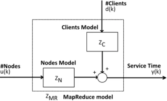
We propose a dynamic model that predicts MapReduce cluster performance, in our case average service time, based on the number of nodes and the number of clients. To the best of our knowledge this is the first dynamic performance model for MapReduce systems. The structure of our model can be seen in Figure 2. Our control input u(k) is the number of nodes in the cluster while the changes in clients d(k) is considered as a measurable disturbance. Our output y(k) is the average service time of a job in the kth time interval. As in the
operating region our system is linear we can apply the principle of superposition to calculate the output:
y(k) = ZC(z)d(k) + ZN(z)u(k) (1)
where ZN is the discrete time model between service time
and the number of nodes and ZCis the discrete time model
between service time and the number of clients.
ZN ZC + + u(k) y(k) d(k) ZMR Nodes Model Clients Model MapReduce model Service Time #Clients #Nodes
Fig. 2. MapReduce control theoretical model. 3.4 Model Identification
Both of the models were identified using step response identification. The observed linearity in the operating region, the lack of overshoot and exponential decay all indicate that the response could be modeled, at least in a first approach, with a first-order linear difference model with deadtime. The parameters of our model are identified using prediction error estimation method. This method has the advantage that it puts an emphasis on the model accuracy in predicting the next observation rather then on its difference from a corresponding statistical model, as it is the case for least square and maximum likelihood
identification methods. Furthermore this method has been shown to provide optimal results (minimal covariance matrix) in the case when the chosen model structure
reflects well the true system, see Ljung (2002). As our
system has large time constants (>300s) we determine that a sampling period of 30 seconds is sufficient. The models are identified as continuous time models and we use the Tustin bilinear transformation to discretize them.
System identification without disturbance The identified
model for the node changes can be seen in Figure 3. A
0 5 10 15 20 25 30 35 40 140 150 160 170 180 Service time (s) Step response Real system Identified system 0 5 10 15 20 25 30 35 40 10 15 20 25 #Nodes Time (min)
Fig. 3. Identification of the undisturbed system. It predicts the effect of nodes changes on job runtime.
step in the number of nodes is used to identify the model between the service time and the number of nodes. The model captures well system dynamics with a fit level of 89%. Equation (2) presents the identified discrete time transfer function of the system without disturbances.
ZN(z) = z−5
−0.17951(z + 1)
z − 0.919 (2)
Disturbance model identification Figure 4 shows the step
responses for the identified and measured systems, in the case of changes in the number of clients.
0 5 10 15 20 25 30 35 160 180 200 220 240 Service time (s) Step response Real system Identified system 0 5 10 15 20 25 30 35 0 5 10 15 20 #Clients Time (min)
Fig. 4. Identification of the disturbance model. It captures the effect of the changes in the number of clients on job runtime.
As we can see, the identified model follows closely the measurements taken from the real system, presenting a 87.94% fit. Equation (3) gives us the discrete time transfer function of the disturbance model:
ZC(z) = z−8
1.0716(z + 1)
z − 0.7915 (3)
Both of identified discrete time transfer functions are stable, first-order systems with their poles inside the unit circle. Therefore the open loop system is inherently stable.
4. CONTROL 4.1 Challenges and motivations
Controlling the performance of MapReduce presents sev-eral specific challenges. One such challenge is represented by the large deadtime (>90s). This is due to the fact that, the effect of adding nodes and clients, is a complex proce-dure and is not instantaneous. Furthermore the implemen-tation we use brings other several specific challenges. For example, as starting and removing nodes always influences the energetic and monetary cost, we need a closed loop response with small, if no, overshoot. Another interesting challenge is that of quantization, since the number of nodes we add or remove must be a positive integer. Finally, as the system performance may vary over time because of the many points of contention, the controller algorithm needs to be robust enough to handle modeling uncertainties.
4.2 Control architecture
A PI controller is chosen as it is well proven that for our system (i.e. a first order system with deadtime - see equation (2)) it is sufficient even if the system is complex, with eventually higher order dynamics, see Guillermo J (2005). Furthermore, a PI feedback controller has well-proven disturbance rejection properties for unmeasured and unmodelled disturbances.
Since we can accurately measure the disturbance we also add a feedforward controller that improves our controls response, as it counteracts the effect of the disturbance before its effects the output. The complete schema of the control architecture is in Figure. 5. The variables used in the figure are defined in Table 2.
ZMR yr(k) ufb(k) uff(k) u(k) e(k) d(k) y(k) + + -ZFF PI controller Feed-forward controller MapReduce System Service time #nodes #clients y(k) Reference service time ZPI
-Fig. 5. MapReduce Control architecture
yr Reference average service time set in the SLA. y System output - average service time of CIs.
u System control input - number of nodes in the system. uf b Control input of the PI controller.
uf f Control feedforward controller. e Error input to the feedback control.
d Disturbance input - number of clients running jobs. ZM R Discrete time MapReduce system model.
ZP I Discrete time PI feedback controller. ZF F Discrete time feedforward controller.
Table 2. Definition of control variables.
4.3 Open loop experiment
Figure 6 shows the baseline open loop experiment where we have no control, only a step increase in the exogenous input. Such a bursty increase in the number of clients occurs frequently in practice, see Kavulya et al. (2010) who analyse a 10 month log production of Yahoo’s super-computing cluster. 0 5 10 15 20 25 30 100 150 200 250 300 Service time (s)
Open loop experiment. 100% more clients are added. Service time (y)
Control reference (yr) SLO threshold 0 5 10 15 20 25 30 5 10 15 20 #Clients Time (min)
Fig. 6. Open loop experiments
In our case we can see that, when 100% more clients are added, the systems service time quickly exceeds the reference threshold defined in the service level agreement. In order to respect the threshold set in the Service Level Agreement (SLA) we employ a PI controller.
4.4 PI Feedback Control
The standard equation of a sampled time PI controller can be seen in equation (4):
uf b(k) = uf b(k − 1) + (Kp+ Ki)e(k) + Kie(k − 1) (4)
The controllers parameters are determined to assure closed loop stability and 0% overshoot. As we would like to avoid a highly aggressive controller the controllers response to the disturbance is somewhat slow. The reason behind this is the minimization of the number of changes in the number of nodes, because of monetary and energetic constraints. Based on these requirements we computed
the value of Kp = 0.0012372 and Ki = 0.25584 for our
controller. Figure 7 shows our controllers response to a 100% change in the number of clients. We can see that as the controller is determined to have a slow settling time, the SLA threshold is breached for a short amount of time but the controller will always take the service time
our reference value. The controller steadily increases the number of nodes until service time recovers. In order to avoid the non compliance with the SLA and to improve the response time of the control a feedforward controller is added. 0 5 10 15 20 25 30 100 150 200 250 300 350 Service time (s)
PI feedback control. 100% more clients are added. Service time (y)
Control reference (yr) SLO threshold 0 5 10 15 20 25 30 0 10 20 30 #Clients Time (min) #Clients (d) 10 20 30 40 50 60 #Nodes #Nodes (u)
Fig. 7. Closed loop experiments - Feedback Control
4.5 Feedforward Control
To improve upon the previous results, a fast feedforward controller is designed to pro-actively reject the disturbance before its effect is observed on the output. The disturbance represents a change in number of concurrent clients. The effectiveness of the feedforward controller depends entirely on the accuracy of the identified model.Most importantly, it does this at the same time the disturbance’s effect presents itself. If the model is 100% accurate the net effect on the response time should be zero, but because of the inherent model uncertainties this is never the case in practice. Our controller is determined using the standard
feedforward formula Zf f(z) = −ZN(z)−1ZC(z) where
Zf f is the discrete time feedforward controller and ZN,
ZC are the discrete time models from Figure 2. The
equation of the computed feedforward controller is given in equation (5). Zf f(z) = z−3 5.9698(z − 0.919) (z − 0.7915) (5) 0 5 10 15 20 25 30 100 150 200 250 300 350 Service time (s)
PI feedback + feedforward control. 100% more clients are added. Service time (y)
Control reference (y r) SLO threshold 0 5 10 15 20 25 30 0 10 20 30 #Clients Time (min) #Clients (d) 10 20 30 40 50 60 #Nodes #Nodes (u)
Fig. 8. Closed loop experiments - Feedback and Feedfor-ward Control
The effect of adding the feedforward control to the already existent feedback controller can be seen in Figure 8. We
can see that the controller response is increased and man-ages to keep the response time below the SLA threshold. Furthermore, the feedback term compensates for all the model uncertainties that were not considered when calcu-lating the feedforward and assures that the steady state error converges to 0.
5. CONCLUSIONS AND FUTURE WORK This paper presents the design, implementation and evalu-ation of the first dynamic model for MapReduce systems. Moreover, a control framework for assuring service time constraints is developed and successfully implemented. First we built a dynamic grey box model that can ac-curately capture the behaviour of MapReduce. Based on this, we use a control theoretical approach to assure perfor-mance objectives. We design and implement a PI controller to assure service time constraints and then we add a feed-forward controller to improve control response time. The control architecture is implemented in a real 40 node clus-ter using a data intensive workload. Our experiments show that the controllers are successful in keeping the deadlines set in the service level agreement.
Further investigations are necessary in some areas and are studied now, such as:
(1) implementing the control framework in an on-line cloud such as Amazon EC2.
(2) improve upon our identification by making it on-line. (3) minimize the number of changes in the control input. Other control techniques such as an event-based con-troller for example are being studied now.
(4) add other metrics to our model such as throughput, availability, reliability.
REFERENCES
Cappello, F., Caron, E., Dayde, M., Desprez, F., Jegou, Y., Primet, P., Jeannot, E., Lanteri, S., Leduc, J., Melab, N., Mornet, G., Namyst, R., Quetier, B., and Richard, O. (2005). Grid’5000: A large scale and highly reconfigurable grid experimental testbed. In Proceedings of the 6th IEEE/ACM International Workshop on Grid Computing, 99–106. Washington, DC, USA.
Cardosa, M., Narang, P., Chandra, A., Pucha, H., and Singh, A. (2011). STEAMEngine: Driving MapReduce provisioning in the cloud. In 18th International Confer-ence on High Performance Computing (HiPC), 1–10. Chen, Y., Alspaugh, S., and Katz, R.H. (2012). Design
insights for MapReduce from diverse production
work-loads. Technical Report UCB/EECS-2012-17, EECS
Department, University of California, Berkeley.
Dean, J. and Ghemawat, S. (2008). MapReduce: simplified data processing on large clusters. Communications of the ACM, 51(1), 107–113.
Guillermo J, S. (2005). PID Controllers for Time-Delay Systems. Birkhauser Boston.
Hellerstein, J.L., Diao, Y., Parekh, S., and Tilbury, D.M. (2004). Feedback control of computing systems. John Wiley & Sons, Inc., New Jersey.
Herodotou, H. and Babu, S. (2011). Profiling,
what-if analysis, and cost-based optimization of MapReduce programs. PVLDB, 4(11), 1111–1122.
Kavulya, S., Tan, J., Gandhi, R., and Narasimhan, P. (2010). An analysis of traces from a production
MapRe-duce cluster. In Proceedings of the 10th IEEE/ACM
International Conference on Cluster, Cloud and Grid Computing (CCGRID), 94–103. Washington, DC, USA. Lin, H., Ma, X., and Feng, W.C. (2012). Reliable
MapRe-duce computing on opportunistic resources. Cluster
Computing, 15(2), 145–161.
Ljung, L. (2002). Prediction Error Estimation Methods. Circuits, systems, and signal processing, 21(1), 11–21. Malrait, L., Marchand, N., and Bouchenak, S. (2009).
Modeling and control of server systems: Application to database systems. In Proceedings of the European Con-trol Conference (ECC), 2960–2965. Budapest, Hungary. Poussot-Vassal, C., Tanelli, M., and Lovera, M. (2010). Linear parametrically varying MPC for combined qual-ity of service and energy management in web service systems. In American Control Conference (ACC), 2010, 3106–3111. Baltimore, MD.
Ren, Z., Xu, X., Wan, J., Shi, W., and Zhou, M. (2012). Workload characterization on a production Hadoop cluster: A case study on Taobao. In IEEE International Symposium on Workload Characterization (IISWC), 3– 13. La Jolla, CA.
Rutten, E., Buisson, J., Delaval, G., de Lamotte, F., Diguet, J.F., Marchand, N., and Simon, D. (2013). Control of autonomic computing systems. Submitted to ACM Computing Surveys.
Sangroya, A., Serrano, D., and Bouchenak, S. (2012). Benchmarking Dependability of MapReduce Systems. In IEEE 31st Symposium on Reliable Distributed Sys-tems (SRDS), 21 – 30. Irvine, CA.
Tian, C., Zhou, H., He, Y., and Zha, L. (2009). A dynamic MapReduce scheduler for heterogeneous workloads. In Proceedings of the 8th International Conference on Grid and Cooperative Computing (GCC), 218–224. Washing-ton, DC, USA.
Tian, F. and Chen, K. (2011). Towards optimal resource provisioning for running MapReduce programs in public
clouds. In IEEE International Conference on Cloud
Computing (CLOUD), 155–162. Washington, DC, USA. Verma, A., Cherkasova, L., and Campbell, R. (2011). Resource provisioning framework for MapReduce jobs with performance goals. In Middleware 2011, volume 7049 of Lecture Notes in Computer Science, 165–186. Springer Berlin Heidelberg.
Vernica, R., Balmin, A., Beyer, K.S., and Ercegovac, V.
(2012). Adaptive MapReduce using situation-aware
mappers. In Proceedings of the 15th International
Conference on Extending Database Technology (EDBT), 420–431. New York, NY, USA.
Wang, K., Lin, X., and Tang, W. (2012). Predator; An experience guided configuration optimizer for Hadoop
MapReduce. In IEEE 4th International Conference
on Cloud Computing Technology and Science,, 419–426. Taipei.
White, T. (2012). Hadoop: the definitive guide. O’Reilly Media, CA.
Xie, D., Hu, Y., and Kompella, R. (2012). On the per-formance projectability of MapReduce. In IEEE 4th In-ternational Conference on Cloud Computing Technology and Science (CloudCom),, 301–308. Taipei.
Xu, L. (2012). MapReduce framework optimization via performance modeling. In IEEE 26 International Paral-lel & Distributed Processing Symposium (IPDPS), 2506– 2509. Shanghai, China.
Yang, H., Luan, Z., Li, W., and Qian, D. (2012). MapRe-duce workload modeling with statistical approach. Jour-nal of Grid Computing, 10, 279–310.
Zaharia, M., Konwinski, A., Joseph, A.D., Katz, R., and Stoica, I. (2008). Improving MapReduce performance in heterogeneous environments. In Proceedings of the 8th USENIX Conference on Operating systems design and implementation (OSDI), 29–42. Berkeley, CA, USA. Zhang, Z., Cherkasova, L., Verma, A., and Loo, B.T.
(2012). Automated profiling and resource management of pig programs for meeting service level objectives. In Proceedings of the 9th International Conference on Autonomic Computing (ICAC), 53–62. San Jose, CA, USA.