The Crystal Structure of Cholesterol Helical
Ribbons
by
Chintan Hossain
Submitted to the Department of Physics
in partial fulfillment of the requirements for the degree of
Bachelor of Science in Physics
at the
MASSACHUSETTS INSTITUTE OF TECHNOLOGY
May 2007
@2007 Chintan Hossain. All rights reserved.
T
heh~
iWt
@WF puolmsh
tb
npel
d
.
idbut pubbly pperd aissbob"i espi
of
theis
wdewent
616sbw wlaupas
m an
MdheW
e h
ws
or herei" maim
Author
Department of Physics
May 11, 2007
6.
/
Certified by..
Professor George B. Benedek
Alfred H. Caspary Professor of Physics and Biological Physics
Thesis Supervisor
A ccepted by ... . ... • ., . ,...
Professor David
E.
Prichard
Senior Thesis Coordinator, Department of Physics
ARcHIVES
I~ASCHUSý-MrS INSTrTT
OF TECHNOLOGY
AUG
0 6 2007
The Crystal Structure of Cholesterol Helical Ribbons
by
Chintan Hossain
Submitted to the Department of Physics on May 11, 2007, in partial fulfillment of the
requirements for the degree of Bachelor of Science in Physics
Abstract
Helical ribbons form in a many multi-component solutions containing sterols similar to cholesterol, but remarkably, almost all the helices have a pitch angle of 110 or 540. The consistent pitch angle of the ribbons may be due to an underlying crystal structure. In order to determine the crystal structure, I undertook x-ray scattering studies of individual helical ribbons taken from two particular solutions: Chemically Defined Lipid Solution and model bile. Using a synchrotron x-ray source I observed Bragg reflections from ribbons with a pitch angle of 110.: From the diffraction patterns, I was able to deduce the parameters of the unit cell. The crystal structure of these ribbons is similar to that of cholesterol monohydrate, with the important difference that the length of the unit cell perpendicular to the cholesterol layers is tripled. Furthermore, I found that adjacent layers are shifted relative to each other along a single direction, and that the shift varies periodically with a period of 3 bilayers. I also found that the growth direction of the crystal is along one of the unit cell axes.
Thesis Supervisor: Professor George B. Benedek
Acknowledgments
I would like to thank George Benedek, Boris Khaykovich, Aleksey Lomakin, and Jennifer McManus for help on this project. I would also like to thank the Argonne National Lab for use of the beamline facilities at the Advanced Photon Source.
Contents
1 Introduction
1.1 Formation of Helical Ribbons . . . . 1.2 Formulation of Reciprocal Space . . . . .
1.3 Theory of Superlattice Modulations . . . . 2 Materials and Methods
2.1 Materials Used ...
2.1.1 Protocol for Preparing Model Bile. 2.2 Preparing Samples ...
2.2.1 Out of Solution ... 2.2.2 In Solution ... 2.3 Diffraction Setup ...
3 Results
3.1 Sample Diffraction Images . . . .
3.2 Data Analysis Program ...
3.2.1 Extracting Bragg Reflections. . . .
3.2.2 Extracting the Direction of c* . . . 3.2.3 Extracting the Magnitude of c* . .
3.2.4 Extracting Components of a* and b
3.2.5 Extracting Components of a* and b
3.2.6 Calculating Errors ...
3.2.7 Final Unit Cell Parameters . . . . .
* Perpendicul * Parallel to 21 . . . . .. . . 21 . . . . . 23 . . . .. . 24 . . . .. . 24 . . . .. . 27 . . . .. 29 33 . . . . . 33 . .. . . . 35 . . . . . 35 . . . . . 36 . . . . . 37 lartoc* . . . 37 c* .. . . . . 39 . . . .. . . . 39 . . . . . 39
3.3 Comparison of Unit Cells ... 40
3.4 Superlattice Modulations ... 41
3.5 Helices from Model Bile In Solution . . . . 41
3.6 Growth Direction . . . . 42
4 Discussion 45 4.0.1 Superlattice Modulations . . . . 45
List of Figures
1-1 Sequence of formation of structures seen in model bile. This image was reproduced from Reference [1] ... 15 1-2 Diagram showing the difference in travel distance for a wave scattered
at IF relative to a wave scattered the origin. The difference in travel distance is the sum of the two segments indicated . . . . 16 1-3 Two dimensional cross-section of a example reciprocal space showing a
reciprocal lattice and an Ewald sphere. The reciprocal lattice vectors
a* and b* and the (1,0,0) and (0,1,0) Bragg reflections are labeled. . 18 2-1 A low pitch helix in CDLC ... 22 2-2 A micro-capillary is threaded through a single turn of a helix so that
it can be lifted out of the solution . . . . 25 2-3 A micro-capillary with a ribbon on it is brought near a polyacrylamide
micro-mount to attach it to the micro-mount . . . . 26 2-4 Two complete samples. The sample on the left is attached to a
micro-mount, and the sample on the right is attached to a nylon loop. . . . 27 2-5 A capillary with a ribbon inside it. The ribbon was drawn into the
capillary using a Cell-Tram pump ... 28 2-6 A sample with a ribbon in solution sealed in a glass capillary. The
ribbon is not as clearly visible in this figure compared to Figure 2-5 because the capillary has been removed from the solution, so light leaving the capillary experiences greater refraction . . . . 30
3-1 Diffraction image from a cholesterol arc. The inset shows a region of the image as it evolves due to crystal rotation. Each frame in the inset corresponds to a crystal rotation angle of 1 degree, and the entire sequence shows a range of 19 degrees of crystal rotation. As the inset shows, each Bragg reflection persists over a range of about 8 degrees of crystal rotation, so the reflections span about 8 degrees in reciprocal space . . . 34
3-2 Spot selection tool selecting a single Bragg reflection. The sequence of frames shows a region of the diffraction image as the crystal is rotated by 18 degrees in intervals of 1 degree. The boxes mark peaks in different images corresponding to a single Bragg reflection . . . . 36
3-3 A histogram showing the distribution of distances between adjacent Bragg reflections along the (h,k) rods. The peak at 0.062 A corresponds to c*. There are peaks at 2c* and 3c* because occasionally one or two Bragg reflections do not appear. The fact that the peak at 3c* is more intense than the peak at 2c* implies that Bragg reflections are usually skipped in pairs... 38
3-4 A region of reciprocal space in which the Bragg reflections follow a pattern of one strong spot followed by two weak spots . . . . 38
3-5 Crystallographic convention for defining the unit cell parameters. The magnitudes of a, b, and ' and the angles between them are specified. The angle between a and b is -y, the angle between b and ' is a, and the angle between d and ' is # ... 40
3-6 A diffraction image taken from a helical ribbon from model bile in so-lution. The dotted line indicates the axis of helical curvature. The diffraction pattern is symmetric about this axis. The top, left half of the image has been covered with boxes indicating the pattern pre-dicted by the unit cell obtained for helical ribbons in CDLC taken out of solution. The predictions match the experimental data, indicating that ribbons in model bile in solution are consistent with the structure obtained from CDLC ribbons. ... 43
Chapter 1
Introduction
The formation of helical ribbons in multi-component lipid solutions is an interesting phenomenon, and poses several questions about the structure and process of formation of the ribbons. Helical ribbons were first discovered in human gallbladder bile, where they form as a precursor to gallstones upon dilution of the bile [2]. Similar ribbons were later found in a variety of solutions containing sterols similar to cholesterol, surfactants, and fatty acids or phospholipids [3]. However, despite the wide variety in composition of the solutions, almost all the ribbons have a pitch angle of either 110 or 540.
Explaining the consistency of the observed pitch angles of poses a challenging problem. Several models have been proposed to explain the structure of the helical ribbons [4, 5, 6, 7, 8, 9, 10, 11]. These models describe the ribbons as being composed of phospholipids arranged into bilayers with the hydrophillic head groups on the outer surface of the ribbons, and the hydrophobic tail groups sandwiched inside the bilayer. The curvature and helical structure of the ribbons is explained using the curvature elasticity model, by minimizing the membrane elastic free energy of ribbon as a function of its curvature [12].
However, these theories do not explain several important features of the helical ribbons. First, the ribbons are observed to have a pitch angle of either 110 or 540 in a wide variety of solutions, while the proposed models predict that the pitch angle varies depending on the composition of the solution. Secondly, the ribbons are composed
primarily of sterols [3], while the proposed theories describe the ribbons as being composed of phospholipids. Thirdly, the thickness of some the ribbons is on the order of microns, as evidenced by colored thin-film interference patterns seen from the ribbons. However, theoretical models predict the thickness of the ribbons to be
the thickness of phospholipid bilayers, which is about 30 A.
An alternative explanation for the structure of the helical ribbons is that it is caused by a crystalline cholesterol structure in the ribbon. This theory explains the results outlined previously, and is also consistent with the fact that helical ribbons are metastable intermediates on the pathway to formation of large cholesterol crystals [1]. Indeed, one theoretical model, outlined in Reference [13], explains the structure of the helices using a crystal model, and is consistent with experimental results. In order to directly determine the crystal structure of the helical ribbons, I undertook X-ray diffraction measurements of the ribbons. Reference [14] contains the manuscript submitted by the group I worked with on this project.
1.1
Formation of Helical Ribbons
Helical ribbons form as precursors to large cholesterol crystals in a many solutions. Crystallization begins when a solution containing sterols, surfactants, and fatty acids or phospholipids is diluted. In an undiluted solution, the sterols are solubilized by micelles, which are spherical structures made of surfactants and phospholipids with the hydrophillic head groups on the outer surface and the hydrophobic groups in the interior. The hydrophobic sterols are contained inside the micelles. The undi-luted solution contains both free surfactants and surfactants contained in micelles in equilibrium. Diluting the solution shifts the equilibrium from primarily micelles to primarily free surfactants. As the micelles break up, they release the sterols they contain, supersaturating the solution with respect to the sterol [1].
Upon dilution, a variety of structures including filaments, helical ribbons, tubules, flat ribbons, and large cholesterol monohydrate crystals form from the solution. The exact structures that form, and the sequence in which they form depend on the
compo-sition of the solution and the concentration of its components. The specific sequence of structures observed in model bile, a solution containing cholesterol, lecithin, and sodium taurocholate, is shown in Figure 1-1.
reaturated
Bile
a4 .W
4 . %%1 % V4 14%4f* -4 % 4% 4 " 4 A \ 4Growth Patterns In Bile
Hlah
PEtch
Low Piiho
4 Helioes
chokesterl
4yM7dt
Figure 1-1: Sequence of formation of structures seen in model bile. This image was reproduced from Reference [1].
1.2
Formulation of Reciprocal Space
The analysis of the data from this experiment relies heavily on the reciprocal space formulation of Bragg diffraction, which is described in this section.
Suppose an electromagnetic wave with wave vector ki incident on a crystal. Every point in the crystal scatters the wave in all directions. Consider all waves scattered in a specific direction. The waves scattered in this direction all have the same wave-vector kf, and the same angle change in angle, defined to be 20 by crystallographic
convention. No significant energy is lost or gained by scattering, so
Iki
=IkAl.
The extra distance traveled by a wave scattered at location f relative to a wave scatteredat the origin ('F=O0) is given by Equation 1.1, which is made clear by Figure 1-2.
As = - (1.1)
Thus, the relative phase of a wave scattered at position f relative to a wave scattered at the origin is given by Equation 1.2, where ' is defined as q'= kf - ki.
< k=lAs = (i - kf) -F = - (1.2)
-k-fr
,ii'
Ilil
Figure 1-2: Diagram showing the difference in travel distance for a wave scattered at F relative to a wave scattered the origin. The difference in travel distance is the sum of the two segments indicated.
The amplitude of the wave scattered from location f' is proportional to g(r-, 20), the scattering cross section per volume at location r' in the crystal. In general, the scattering cross section depends on the scattering angle, 20. Combining g(f', 20) with the phase difference given in Equation 1.2, the complex amplitude of a wave scattered from location f is given by Equation 1.3.
A oc g(r', 20)e-`' (1.3)
Integrating over the total volume of the crystal, the total amplitude scattered in the direction of kf is given by Equation 1.5.
A oc f g(, 20)e-i7Fd3f (1.4)
Suppose that the crystal has a unit cell with sides given by vectors a, b, and
c. Then ' can be written as F = nfa + nb + +cc+cell, where n, b, and no
specify a specific unit cell, and FeIL specifies the location in the unit cell. Because of periodicity of the crystal, g(nad + nb+ nlc+ Fcei, 20) = g(Feu, 20). Substituting
f= nfaa+nb+ncbb +rcel into Equation 1.3 gives Equation 1.5. Note that the integral in Equation 1.5 is only over a single unit cell.
A
oc
e-i (na nb +nc)J+
flg(fla,
20)e-i~ Fe1d3cell
(1.5)
na, nb,nc unitcell
Equation 1.5 separates into the product of two terms. The right term depends on the scattering density within the unit cell, and is known as the structure factor. The left hand term depends only on the unit cell dimensions, and not on the distribution of scattering density inside the unit cell. Let us focus on this term. For an infinite crystal, this term is non-zero only if Equations 1.6, 1.7, and 1.8 hold for any integers
h, k, and 1.
q = 2rh (1.6)
q-b = 27rk (1.7)
• - = 27rl (1.8)
These equations can be satisfied by q = ha + kb* + 1 , where ac, b*, and c are given by Equations 1.9, 1.10, and 1.11
bxah a = 27r (1.9) •- (bx cla
b* = 2
(1.10)
b -(E'x d)
axb c( = 2 (1.11)Therefore, the values of q that produce Bragg reflections form a lattice, known as a reciprocal lattice, in the space of possible q, known as reciprocal space. Each Bragg reflection has a unique set of (h,k,1) indices. For a specific value of ki, the possible values of ' resulting from all kf with the same magnitude as ki form a sphere centered around -ki with a radius of
Ikil.
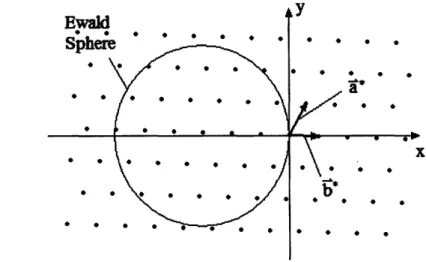
This sphere is known as an Ewald sphere. Figure 1-3 shows a two dimensional cross-section of an example reciprocal space with a reciprocal lattice and Ewald sphere.Figure 1-3: Two dimensional cross-section of a example reciprocal space showing a reciprocal lattice and an Ewald sphere. The reciprocal lattice vectors a* and b* and the (1,0,0) and (0,1,0) Bragg reflections are labeled.
In an X-ray diffraction experiment, each point on the X-ray detector corresponds to a point on the Ewald sphere. A Bragg reflection will be observed if the Ewald sphere crosses a point in the reciprocal lattice. Rotating the crystal rotates the reciprocal lattice. Alternatively, with a simple coordinate transformation, rotating
the crystal rotates the Ewald sphere about the origin while holding the reciprocal lattice fixed. This new set of coordinates is referred to crystal coordinates, because the crystal is fixed in the new coordinate system. Therefore, the entire reciprocal space in crystal coordinates can be constructed by taking a series of images over a range of crystal rotation angles. Near the origin, the Ewald sphere is close to a flat plane, so the crystal only needs to be rotated over a range of 180' to construct the reciprocal lattice near the origin. For an ideal, infinite crystal, as described in this section, the Bragg reflections have zero volume in reciprocal space. However, in a real crystal the Bragg reflections will have a non-zero width in reciprocal space, so a finite series of images is sufficient to locate all the Bragg reflections.
1.3
Theory of Superlattice Modulations
We found evidence for superlattice modulations in the helical ribbons, so in this section I will formulate the diffraction pattern obtained from a crystal with superlat-tice modulations. More specifically, this section considers modulations in which the crystal planes are shifted along single direction with the amount of the shift varying periodically along the direction perpendicular to the planes. Suppose that the ab planes shift by some amount along the d direction, where d is a unit vector. Let the amount of the shift vary periodically with period m, where m is an integer. Let the values Xo, x1, x2,... xm-1 be the magnitudes of the shifts of planes defined by
c = 0, 1, 2,... m - 1. Because of periodicity, the plane with c=m+n has the same shift as the plane with c=n for any n. Then, the equation for r' in terms of rcen
changes to = n.d + nbb + F nC+Xn nod+ rcell
Inserting this into Equation 1.3, and using the fact that g(naa+ nbb+ nc+ Xncd+
frce, 20) = g(F'ceu, 20) gives Equation 1.12.
A cc bc*Lf e- '(n +n + + d
Lni
gcel , 1 120)e-i'rceLd3jfe' (1.12)Once again, the intensity factors into two terms, and we will ignore structure factor term. The left term can be split into 3 pieces, as shown in expression Expression 1.13.
Se-in.Ta E inqb E e-i(nc,+xncd) (1.13)
na nb nc
The left two sums are unchanged from the case with no superlattice modulations, and lead to the conditions in Equations 1.6 and 1.7. If q'-d = 0, then the third sum is also unchanged, and recovers the condition in Equation 1.8 So, in the plane perpendicular to d in reciprocal space, the reciprocal lattice is unchanged. However, if q'. d 0 the third sum leads to a different condition. If we set n, = fm + g for
integers f and g, with 0 < g < m, the sum can be rewritten as Expression 1.14, using the fact that Xfm+g = xg.
m--1
e- i m•• e-i~ (g+xgd (1.14) f g=0
In general, the right term depends in the specific values of xg, so no conclusions can be made about it (except when d = 0, but this case was discussed earlier). The left hand term is non-zero only if Equation 1.15 holds.
.- (mc .= 27rl (1.15)
Equation 1.15 is almost identical to Equation 1.8, but with ' replaced with md. This makes good physical sense, because a unit cell with dimensions a, b, and mc can be drawn covering an entire period of superlattice modulation. From this we expect a reciprocal lattice with dimensions a , b*, and c/m. Therefore, there are intermediate
spots seen along the c direction. Between each (h,k,1) and (h,k,l+1) for a crystal with no superlattice modulations, m-1 new spots are inserted if there are superlattice modulations. However, intermediate spots do not appear everywhere. Specifically, they do not appear when '- d=0, so the intermediate spots are not seen in a plane
Chapter 2
Materials and Methods
2.1
Materials Used
Helical ribbons were obtained from two different solutions. The first solution was Chemically Defined Lipid Concentration (CDLC), commercially available from GIBCO. CDLC is a water solution containing non-ionic surfactants (Pluronic F-68 and Tween 80), a mixture of fatty acids, and cholesterol. We do not know the protocol for preparing CDLC.
The second solution was model bile, prepared in the lab from a mixture of choles-terol, sodium taurocholate, and 1,2-dioleoyl-glycero-3-phosphocholine (DOPC) ac-cording to the protocol described in Section 2.1.1.
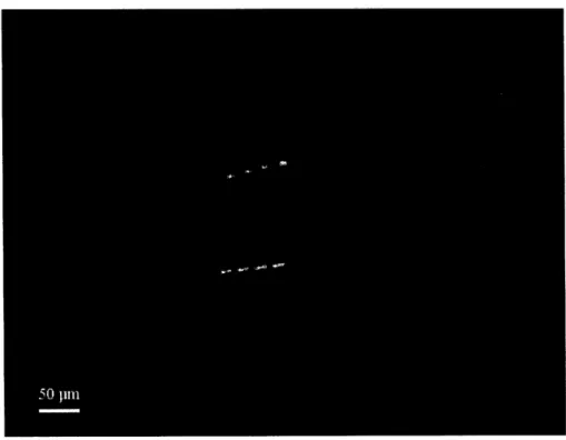
CDLC contains a very high concentration of structures, whereas model bile con-tains far fewer structures. Most of the helical ribbons in CDLC are low pitch, while most of the helical ribbons in model bile are high pitch. The helical ribbons in CDLC have a larger average length, radius, and thickness than the ribbons in model bile. However, the low pitch helices in model bile tend to be significantly larger than the high pitch helices in model bile. The size of the ribbon is very important for sample preparation, as described in Section 2.2. An example of a low pitch helix in CDLC is shown in Figure 2-1.
Figure 2-1: A low pitch helix in CDLC.
2.1.1
Protocol for Preparing Model Bile
Model bile was prepared using a stock solution of DOPC containing 20 mg/mL in chlo-roform obtained from Avanti Polar Lipids, cholesterol powder obtained from Sigma-Aldrich, and sodium taurocholate powder obtained from Sigma-Aldrich. The protocol for preparing model bile was obtained from Reference [2].
The model bile was prepared according to the following procedure:
1. Cholesterol was recrystallized in a solution of 95% ethanol and 5% water to improve the purity.
2. Cholesterol was dissolved in chloroform to make a stock solution with a concen-tration of 1 mg/mL.
3. Sodium taurocholate was dissolved in methanol to make a concentration of 100 mg/mL.
4. The stock solutions were mixed to make a solution with DOPC, and cholesterol in a 97.5:0.8:1.7 molar ratio and of 70 mg.
5. The solution was dried under argon to form a lipid film. 6. The lipid film was resuspended in 1 mL of a solution
methanol in a 2:1 ratio by volume.
a stock solution with
sodium a total
taurocholate, solute weight
with chloroform and
7. The solution was dried under argon again.
8. The lipid film was placed in a vacuum lyophilizer to dry completely overnight. 9. The lipid film was suspended in 1 mL of ddH20 filtered with a 0.22 Am filter.
10. The solution was heated to 600C for 1 hour to dissolve the lipid film completely. 11. The solution was supersaturated by adding 5 mL of filtered ddH20 to bring the
12. The solution was filtered to remove any remaining impurities.
13. The solution was placed an incubator for 5 days to allow crystals to grow. During the growth period, the solution was viewed under a microscope at least once a day to check for crystal structures.
2.2
Preparing Samples
Samples were prepared in two ways: in solution and out of solutions. Samples pre-pared out of solution were removed from the liquid, whereas samples prepre-pared in solution were never removed from the liquid.
2.2.1
Out of Solution
Samples were prepared out of solution by lifting ribbons out of solution using micro-capillaries and placing them on nylon loops or polyacrylamide micro-mounts. The micro-capillaries were obtained from Eppendorf, the nylon loops were obtained from Hampton Research, and the micro-mounts were obtained from MiTeGen. The nylon loops and micro-mounts were attached to magnetic bases to allow for easy attachment and removal at the X-ray beamline.
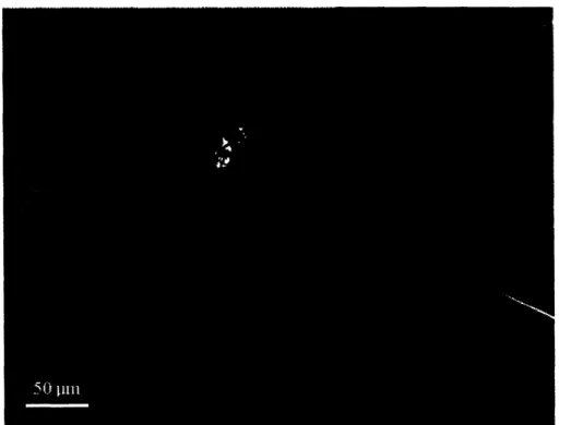
To prepare a sample, a droplet of CDLC was placed under a microscope. The ribbons have an index of refraction similar to that of the solution, so the microscope slide was lit obliquely to make the ribbons visible. The lighting stage was attached to a micromanipulator to allow the droplet of CDLC to be moved. A micro-capillary was attached to another micromanipulator and lowered into the droplet. After choosing a suitable ribbon, the capillary was threaded through a single turn of the helix, and slowly raised out of the solution. Figure 2-2 shows a capillary threaded through a single turn of a helix to prepare to raise it out of the solution
Care must be taken while raising the ribbon out of solution, because the ribbon is very delicate, and can easily be broken by surface tension. Only thick helices are strong enough to withstand the surface tension without breaking. Model bile cannot
Figure 2-2: A micro-capillary is threaded through a single turn of a helix so that it can be lifted out of the solution.
be used to prepare samples out of solution because all the ribbons in model bile are too small to be taken out of solution.
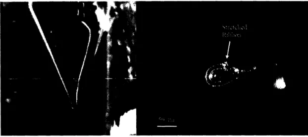
After the ribbon was taken out of the solution, a nylon loop or micro-mount was placed on a third micromanipulator. For samples prepared for low temperature, the loop was covered in a thin film of cryoprotectant oil. The capillary and loop were then brought near each other, as shown in Figure 2-3, and the ribbon was placed across the loop. Figure 2-4 shows two completely prepared samples, with one on a nylon loop and one on a micro-mount. The samples prepared for low temperature were then dipped in liquid nitrogen to cool them to 77 K.
Figure 2-3: A micro-capillary with a ribbon on it is brought near a polyacrylamide micro-mount to attach it to the micro-mount.
Samples prepared out of solution have the advantage of a lower background due
50
Figure 2-4: Two complete samples. The sample on the left is attached to a micro-mount, and the sample on the right is attached to a nylon loop.
to the small amount of liquid and glass in the beam. However, removing samples from the solution can damage them, and ribbons taken out of solution are no longer in their native environment, so their structure may change.
2.2.2
In Solution
To take measurements of helical ribbons in their native environment, some samples were prepared in solution. In this configuration, the ribbons were coiled into their natural shape, rather than stretched flat, as they were in the out-of-solution con-figuration. This was done using hollow Cell-Tram capillaries from Eppendorf. The Cell-Tram capillaries are made of glass, and have an inner diameter of 100 p/m, and have a tapered opening which is narrow near the tip and wide in the body of the capillary. The capillary was attached to an Eppendorf Cell-Tram pump, which can hydraulically push liquid into and out of the capillary. The capillary holder was at-tached to a micromanipulator to allow it to be moved precisely. The capillary was inserted into the solution, and a helix was drawn into the capillary using the pump. Figure 2-5 shows an image of a capillary with a ribbon inside it.
Figure 2-5: A capillary with a ribbon inside it. The ribbon was drawn into the capillary using a Cell-Tram pump.
unmodified capillary. To solve this problem, I filed off part of the tip to widen the opening. This was done by holding the capillary close to the tip to prevent it from bending excessively and filing off the tip using the flat side of a capillary cutter. The capillaries are very delicate, so the tip must be filed gently by applying very little pressure. After filing the tip to the desired opening width, the capillary was washed to remove any glass particles on the capillary. This was done by inserting the capillary into a droplet of ddH20 and pumping water into and out of the capillary vigorously
using the Cell-Tram pump.
After the a ribbon was drawn into the capillary, the capillary was raised out of the solution. The tip of the capillary was covered with Paratone oil to prevent evaporation of solution from the tip of the capillary. The capillary was then removed from the capillary holder by scratching it using a capillary cutter and then breaking it at the point of the scratch. A small amount of sealing wax was inserting into the back of the capillary, and the capillary was slid onto a magnetic base. The capillary was then heated locally for a fraction of a section by a solder gun to melt the wax and seal the back of the capillary. This was done to prevent evaporation of liquid from the back of the capillary. Care was taken while heating the capillary, because heating the solution causes the ribbons to melt. The solder gun was heated to a high temperature and touched to the capillary briefly to heat the capillary locally. Figure 2-6 shows the tip of a completed sample.
For samples prepared in solution, the liquid and glass create a lot of background scattering. The background was greatly reduced by taking an image with the beam aimed away from the ribbon but still passing through glass and liquid. This image was subtracted from the diffraction image taken by aiming the beam directly at the ribbon, thus subtracting away most of the background.
2.3
Diffraction Setup
Diffraction experiments were carried out at the Advanced Photon Source at Argonne National Lab. The Sector 31 (SGX-CAT) protein crystallography beamline was used
Figure 2-6: A sample with a ribbon in solution sealed in a glass capillary. The ribbon is not as clearly visible in this figure compared to Figure 2-5 because the capillary has been removed from the solution, so light leaving the capillary experiences greater refraction.
for measurements. The samples were held in the beam by magnetic bases, and motors controlled the position and orientation of the sample. A horizontal, monochromatic beam with photon energy 12.66 keV (A = 0.98A1) was directed at the sample. Dif-fracted x-rays were detected using a CCD detector (MAR 165). The cross section of the beam was set to 50m x 50m for some samples and 100pm x 100pm for oth-ers. During each measurement, the crystal was rotated with constant angular speed by an angle of 1800 degrees. Images were read from the CCD every 10 or 20. The resulting set of images was later used to construct the reciprocal lattice, as described in Section 1.2.
Low temperature samples were kept at 100 K using a cryostat, which blows cold nitrogen evaporating from a dewar of liquid nitrogen over the sample.
Chapter 3
Results
3.1
Sample Diffraction Images
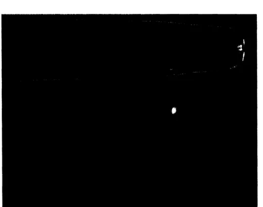
Figure 3-1 shows an example diffraction image cholesterol ribbon. This ribbon was taken out of CDLC, and was not fully helical, but rather a thick, curved arc. These arcs are the easiest structures to take measurements on, because they have a large volume, and thus produce more intense diffraction patterns than fully helical ribbons, and they are easy to remove from the solution due to their thickness. This particular arc was measured at 100 K.
The diffraction image shows a clear lattice of Bragg reflections. Some of these Bragg reflections from tight clusters. The inset of Figure 3-1 shows the evolution of one of these clusters as the crystal is rotated by successive angles of 1 degree over a range of 19 degrees. This corresponds to rotating the Ewald sphere over a range of 19 degrees. As the inset shows, each Bragg reflection persists over a range of crystal angles of about 8 degrees, which implies that the Bragg reflections are elongated in the axial direction in reciprocal space.
The most likely cause for the elongation of the spots is that the ribbon is curved by several degrees, even when stretched across a loop. If the radius of curvature is much longer than the size of the unit cell, as it is for the ribbons, the crystal can be considered to be many small crystals with different orientations, each of which will produce a reciprocal lattice at a different orientation. The combined pattern from
Figure 3-1: Diffraction image from a cholesterol arc. The inset shows a region of the image as it evolves due to crystal rotation. Each frame in the inset corresponds to a crystal rotation angle of 1 degree, and the entire sequence shows a range of 19 degrees of crystal rotation. As the inset shows, each Bragg reflection persists over a range of about 8 degrees of crystal rotation, so the reflections span about 8 degrees in reciprocal space.
all the crystals is a reciprocal lattice with the Bragg reflections smeared in the axial direction about the axis of curvature.
3.2
Data Analysis Program
Available crystallographic software cannot be used analyze our data, because the Bragg reflections in our data span several degrees, and also because the number of visible spots is small. To analyze the data, I programmed a tool that constructs the location of each Bragg reflection in reciprocal space from the images and then determines the lattice dimensions from the points in reciprocal space.
3.2.1
Extracting Bragg Reflections
The raw data that the program takes as input is a series of images taken from a single crystal with the crystal rotation angle varying over a range of 180 degrees. Each image provides a slice of reciprocal space, as described in Section 1.2. Extracting the location of Bragg reflections from these images is a challenge because each Bragg reflection spans several images.
To extract the location of the Bragg reflections in reciprocal space, I programmed a tool that allows the user to manually select the peaks that correspond to a Bragg reflection. Then, the program extracts the location of the Bragg reflection from the location of the peaks. Figure 3-2 shows the spot selection tool being used to select the peaks corresponding a single Bragg reflection. The Bragg reflection produces a peak in every image over a range of 8 degrees.
After the peaks are selected, the program subtracts the local background around each peak, and then determines the the location of each peak by averaging the pixel locations weighted by intensity. Then, it determines the average crystal rotation angle by averaging the rotation angles of the images, weighted by the integrated intensity of the peaks. It also determines the average peak location by averaging the peak location over all the images, weighted by integrated peak intensity. From the average peak location, the location on the Ewald sphere can be determined. Then, the location can
Figure 3-2: Spot selection tool selecting a single Bragg reflection. The sequence of frames shows a region of the diffraction image as the crystal is rotated by 18 degrees in intervals of 1 degree. The boxes mark peaks in different images corresponding to a single Bragg reflection.
be transformed into crystal coordinates by rotating by the negative of the average crystal angle. By repeating for all Bragg reflections that can be resolved, the location of the Bragg reflections in reciprocal space can be determined. The spot selection program was programmed so that multiple Bragg reflections can be selected at once. When doing so, the program ensures that each pixel is only grouped into one peak. This is done by assigning pixels to peaks using a nearest neighbor algorithm. This method is very useful for distinguishing Bragg reflections which are close to each other.
Not all visible Bragg reflections can be resolved, because the Bragg reflections overlap in certain locations of reciprocal space. For the thick cholesterol arc imaged in Figure 3-1, approximately 100 spots were resolved. The spots formed a rectangu-lar lattice in reciprocal lattice. The unit cell of the reciprocal lattice had two long dimensions and one short dimension.
3.2.2
Extracting the Direction of c*
Determination of the reciprocal unit cell from the reciprocal lattice shown was done in several steps. First, I extracted c*, defined to be the shortest reciprocal space unit cell dimension. This was done by considering the set of Bragg reflections with a given value of h and k. These spots form a rod in reciprocal space. To determine the direction of c*, the program calculates the vector difference between adjacent spots along this rod, and then averages the vectors obtained from all rods. The direction of this vector is the calculated c* direction. Although the values of h and k are
not explicitly known at this point, the Bragg rods can be easily identified because c*<<a* and c*<<b*. The program finds the set of vectors connecting adjacent spots by connecting each spot to it's nearest neighbor with the restriction that each spot can be connected to a maximum of two spots, there can only be one vector connecting each pair of spots, and the length of the vector must be less than a maximum value. This is repeated until no more connections can be made. The maximum value in the last condition is set to be less than a* and b* to ensure that spots with different h,k are not connected.
3.2.3
Extracting the Magnitude of c*
To find the length of c* I took the vectors differences between adjacent spots in each h,k rod and projected them onto a vector along the c* direction. The distribution of distances obtained from this procedure are plotted in Figure 3-3. There are major peaks at 0.062 A and 0.18 A. There is also a minor peak at 0.12 A. From this we can deduce that c*=0.062A. The peaks at 0.12 A and 0.18 A occur because occasionally one or two Bragg reflections do not appear, resulting in a vector of length 2c* or 3c* connecting two adjacent spots. The fact that the peak at 3c* is much larger than the peak at 3* implies that spots are usually skipped in pairs.
An explanation for why spots are usually skipped in pairs can be found by looking at the spot intensities. Figure 3-4 shows a region where the Bragg reflections follow a pattern of a strong spot followed by two weak spots. In certain areas, the weak spots may be too weak to resolve. In these areas, two spots will be skipped, resulting in a vector of length 3c*.
3.2.4
Extracting Components of a* and b* Perpendicular to
c*
Next, the components of a* and b* perpendicular to c* were found. This was done by projecting all the spots in reciprocal space into the plane perpendicular to c*. After projections, these spots form a 2 dimension lattice with lattice vectors equal to the
20 O CL 0•
E
z
00.00 0.03 0.06 0.09 0.12 0.15 0.18 0.21 0.24 0.27
Soot
seoaration in reciDrocal soace (AW)
Figure 3-3: A histogram showing the distribution of distances between adjacent Bragg reflections along the (h,k) rods. The peak at 0.062 A corresponds to c*. There are peaks at 2c* and 3c* because occasionally one or two Bragg reflections do not appear. The fact that the peak at 3c* is more intense than the peak at 2c* implies that Bragg reflections are usually skipped in pairs.
Figure 3-4: A region of reciprocal space in which the Bragg reflections follow a pattern of one strong spot followed by two weak spots.
components of a* and b* perpendicular to c*. These lattice vectors were found by doing a least squares fit of the a* and b* onto the measured data. The mean squared error was calculated by averaging the square of the distance between each data point and the closest point in the lattice formed by the chosen a* and b*. The values of a* and b* were adjusted to minimize this error.
3.2.5
Extracting Components of a* and b* Parallel to c*
Finally, the components of a* and b* parallel to c* were found. This was done by a least squares fit similar to the one done in Section 3.2.4. The mean squared error was calculated by averaging the square of the distance between each point and the closest predicted spot. The values of a* and b* parallel to c* were adjusted to minimize the mean squared error.
3.2.6
Calculating Errors
To calculate the errors, I first indexed the spots by assigning the h,k,l indices of the closest predicted spot to each experimental spot. Next I calculated the root mean squared error between the actual spot and predicted spots both along c* and perpendicular to c*. The error perpendicular to c* was divided by V2 to give the error per dimension.
3.2.7
Final Unit Cell Parameters
The final step of the analysis was to invert the reciprocal space unit cell to give the real space unit cell. The equations for inverting the unit cell are identical to Equations 1.9, 1.10, and 1.11, but with the real space and reciprocal space vec-tors switched. The most convenient way of expressing the unit cell dimensions is to specify the magnitudes of a, b, c, and the angles between. Figure 3-5 shows the crystallographic convention for defining the three angles. The errors in a, b, and c were calculated by assuming that a and a* have the same percent error, b and b* have the same error, and c and c* have the same percent error. The percent errors
in the angles were determined by taking the rms-average of the percent errors in the two sides next to that angle. For example, the percent error in -y is the rms-average of the percent errors in a and b.
p
pU
Figure 3-5: Crystallographic convention for defining the unit cell parameters. The magnitudes of a, b, and ' and the angles between them are specified. The angle
between a and b is -y, the angle between b and ' is a, and the angle between a and ' is 0
3.3
Comparison of Unit Cells
For the thick cholesterol arc at 100 K described in Section 3.1, the unit cell para-meters were a=(12.00.2)A, b=(12.00.2)A, c=(102±5)A, a=(89±3)o, ,3=(97±3)o,
-y=(101.1±1.7)0. Measurements were also taken on a thinner, truly helical low-pitch ribbon at room temperature also taken out of CDLC. The unit cell parameters for this crystal were a=(12.1±0.4)A, b=(12.1±0.4)A, c=(102=5)A, a=(90±3)o, 3=(97±3)o, y7=(102±2)0. These two lattices are identical to within the experimental errors. For comparison, the lattice dimensions for cholesterol monohydrate (ChM) are a=12.39A, b=12.41A1, c=34.36A1, a=90.04, /3=98.10, -=100. 8 0. All the unit cell parameters for
the helical ribbons match the unit cell parameters for ChM except for c. The value of c for the helical ribbons is 3 times the value of c for cholesterol monohydrate. This
/ 4
y
I\
t,
implies that the unit cell for helical ribbons is 3 ChM unit cells stacked on top of each other along the c direction, and that the structure of the ribbons may be the same as the structure of ChM, but with a superlattice modulation.
3.4
Superlattice Modulations
If we examine the h,k rods for the diffraction images, we see that there are no inter-mediate spots in rods corresponding to h = -k. The spacing between adjacent Bragg
reflections along the (h,-h) rods is 3c*, which is identical to the spacing that would be expected for ChM. As described in Section 1.3, this implies that the superlattice modulation consists of shifts perpendicular to the plane in which there are no inter-mediate spots. For the helices, there are no interinter-mediate spots in the (h, -h, 1) plane, so the direction of the shifts is along the ' + b direction.
3.5
Helices from Model Bile In Solution
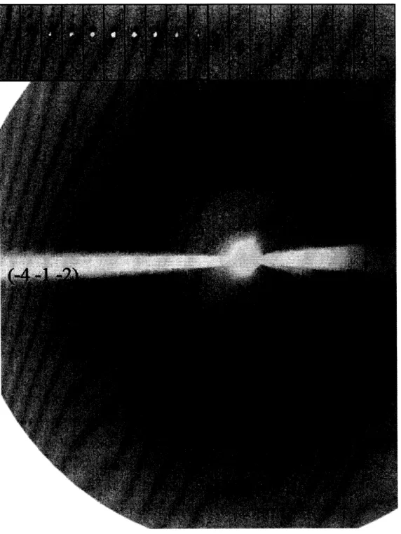
In addition to making measurements on ribbons from CDLC taken out of solution, I took measurements for a model bile ribbon in solution. For a sample in a capillary, it is difficult to aim the beam at the ribbon, because it is nearly invisible once it is sealed in the capillary, and also because the capillary has a large thickness. For these reasons, we could only take one image from the sample. Also the spot intensity was low compared to the background noise, even after subtraction, so not many spots could be resolved. Also, for a fully helical ribbon the curvature angle of the crystal is 360', so the Bragg reflections are stretched into circles instead of Bragg arc. For these reasons, the unit cell parameters could not be extracted from the raw data. Instead, I compared the diffraction image to the pattern predicted using the unit cell extracted from ribbons in CDLC, to determine if the image is consistent with the unit cell found using ribbons from CDLC out of solution.
Figure 3-6 shows the image obtained from the ribbon in model bile. The dotted line shows the axis of helical curvature. The Bragg reflections form circles around
this axis in reciprocal space, so the observed diffraction pattern will be symmetric about the axis of curvature. Half of the image on one side of the dotted line has been covered with boxes marking the location of spots predicted by the unit cell from ribbons in CDLC. As can be clearly seen, the image matches the predictions of the unit cell for ribbons in CDLC. This indicates that fully helical ribbons in model bile also have a structure similar to ChM but with superlattice modulations.
3.6
Growth Direction
The helical ribbon are much longer along one direction compared to the other two directions. If a helical ribbon is stretched out, it's length will be at least an order of magnitude larger than it's width and thickness. This indicates that the crystals grow primarily along one direction. This growth direction can be compared to the unit cell by noting the orientation of the crystal on the sample holder before it is placed into the beamline, and then comparing the orientation of the crystal to the orientation of the diffraction patterns. By doing this, we observe that the growth direction is along the b direction for low pitch helices.
The fact that the pitch angle of the helices is 110 indicates that the growth di-rection is offset from the plane perpendicular to the curvature axis by 110. In other words, the growth direction is offset from the axis of curvature by 1010, indicating that the axis of curvature is also along a crystal axis.
Figure 3-6: A diffraction image taken from a helical ribbon from model bile in solution. The dotted line indicates the axis of helical curvature. The diffraction pattern is symmetric about this axis. The top, left half of the image has been covered with boxes indicating the pattern predicted by the unit cell obtained for helical ribbons in CDLC taken out of solution. The predictions match the experimental data, indicating that ribbons in model bile in solution are consistent with the structure obtained from CDLC ribbons.
Chapter 4
Discussion
4.0.1
Superlattice Modulations
The unit cell of helical ribbon crystals is similar to that of cholesterol monohydrate (ChM) crystals. The unit cell of cholesterol monohydrate has 8 cholesterol molecules in a bilayer configuation with the molecules aligned with their long axis along the c direction. In between the two layers of cholesterol molecules, there is a plane with 8 hydrogen-bonded water molecules parallel to the ab-plane [15, 16]. The values of a, b, and 7-y for helical ribbons are very close to those for ChM. Also, the molecules in the ChM unit cell have translational pseudosymmetry in the ab-plane, which causes the structure factor to be 0 when both h and k are odd [17]. In our diffraction patterns for helical ribbons, we see the same pattern of Bragg reflections with odd h and odd k vanishing. These observations indicate that helical ribbons likely have the same configuration of cholesterol and water molecules in the ab-plane ChM.
The key difference between the helical ribbon crystals and ChM crystals is the arrangement of planes relative to each other. ChM crystals have a crystal structure that repeats every bilayer, resulting in a unit cell for which the length of c is approx-imately equal to two cholesterol molecules. However, helical ribbons have a unit cell that has a value of c three times the value for ChM. This indicates that the arrange-ment of planes in helical ribbons has a period of 3 bilayers, or 6 cholesterol molecules. We were able to determine the direction of the relative shift between planes from
our data. We observed that spots separated by c* do not appear in the (h,-h, 1) plane, which indicates that the planes are shifted relative to each other along the d|b direction.
One possible explanation for the relative shift of planes is the curvature of the helices. Due to the curvature, the length of the outer surface of the ribbon is longer than the length of the inner surface of the ribbon, so a periodic slippage of the inner and outer layers will occur. If this is the case, the direction of slippage, d'
+
b, shouldbe perpendicular to the axis of curvature.
Another possible explanation is that there is a different pattern of water molecules between layers, altering the registration of the bilayers. Such a structure is observed in the cholesterol derivative stigmasterol [18]
Recent studies of cholesterol crystals on the air-water interface [18, 19], as well as diffraction electron microscopy studies of cholesterol films in bile [20] provide insight into the pathway by which helical ribbons may be formed. Both studies show that cholesterol crystals which are only a few molecular layers thick have rectangular unit cell, with a = 10 and b = 7.5 A. As the thickness increases, the rectangular unit cell transforms into the triclinic unit cell of bulk ChM [19]. As the unit cell changes, so does the hydrogen-bonding arrangement of the water molecules interleaving the cholesterol layers. In the triclinic ChM, the mesh of the hydrogen bonds is relatively isotropic, while in the rectangular cell crystals the hydrogen bonds generate a stripe-like network, which is oriented along b [19]. As these initial rectangular strips grow thicker, the arrangement of cholesterol layers converts to the lattice of ChM, which we observe. It is conceivable that, during the growth process, the re-arrangement of water molecules between layers lags behind the rearrangement of cholesterol molecules and produces a hybrid structure showing the superlattice modulation we observe along the c direction.
4.0.2
Pitch Angle
We have demonstrated that the helical ribbons having pitch angle of 110 in CDLC and model bile are constituted of coiled single crystal strips. These strips have a crystal
structure very similar to that of cholesterol monohydrate. The essential difference between these two structures is in the tripling of the size of the unit cell along the c axis for our helices. The plane of the strip lies in the ab-plane, while the direction of preferred growth, i.e. the long edge of the strip lies along the b-axis. Since the angle between a and b-axes is 1010, the angle between the perpendicular to the edge of the ribbon and the a-axis is 110, which coincides with the observed pitch angle. Thus, it appears that the preferential bending direction in low pitch helices is along the a crystallographic axis.
Bibliography
[1] Chung DS, Benedek GB, Konikoff FM, and Donovan JM. Proceedings of the
National Academy of Sciences, 90:11341-11345, 1993.
[2] Konikoff FM, Chung DS, Donovan JM, Small DM, and Carey MC. Journal of
Clinical Investigation, 90:1155-1160, 1992.
[3] Zastavker YV, Asherie N, Lomakin A, Pande J, Donovan JM, Schnur JM, and Benedek GB. Proceedings of the National Academy of Sciences, 96:7883-7887, 1999.
[4] Yager P and Schoen PE. Molecular Crystals and Liquid Crystals, 106:371-381, 1984.
[5] Nakashima N, Asakuma S, and Kunitake T. J Am Chem Soc, 107:509-510, 1985. [6] Georfer JH, Singh A, Price RR, Schnur JM, Yager P, and Schoen PE. J Am
Chem Soc, 109:6169-6175, 1987.
[7] Fuhrhop JH, Schnieder P, Boekema E, and Helfrich W. J Am Chem Soc, 110:2861-1867, 1988.
[8] Thomas BN, Corcoran RC, Cotant CL, Lindermann CM, Kirsch JE, and Persi-chini PJ. J Am Chem Soc, 120:12178-12186, 1998.
[9] Thomas BN, Lindermann CM, and Clark NA. Physics Review E, 59:3040-3047, 1999.
[10] Servuss RM. Chem Phys Lipids, 46:37-41, 1988. 49
[11] Schnur JM. Science, 262:1669-1676, 1993.
[12] Helfrich W. Z Naturforsch, C, J Biosci, 693-703:1669-1676, 1973.
[13] Smith B, Zastavker YV, and Benedek GB. Physics Review Letters, 87:278101, 2001.
[14] Khaykovich. to be published in Proceedings of the National Academy of Sciences, 2007.
[15] Craven BM. Nature, 260:727-729, 1976.
[16] Craven BM. Handbook of Lipid Research, Vol. 4, The Physical Chemistry of Lipids, pages 149-182. Plenum Press, New York, small dm edition, 1986.
[17] Craven BM. Acta Cryst, B35:1123-1128, 1979.
[18] Rappaport H, Kuzmenko I, Lafont S, Kjaer K, Howes PB, Als-Nielsen J, Lahav M, and Leisorwitz. Biophys J, 81:2729-2736, 2001.
[19] Solomonov I, Weygand MJ, Kjaer K, Rapaport H, and Leiserowtiz L. Biophys
J, 88:1809-1817, 2005.
[20] Weihs D, Schmidt J, Goldiner I, Damino D, Rubin M, Talmon Y, and Konikoff FM. J Lipid Res, 46:942-948, 2005.
![Figure 1-1: Sequence of formation of structures seen in model bile. This image was reproduced from Reference [1].](https://thumb-eu.123doks.com/thumbv2/123doknet/14526656.532565/15.918.179.779.271.699/figure-sequence-formation-structures-model-image-reproduced-reference.webp)