HAL Id: hal-02971329
https://hal.inrae.fr/hal-02971329
Submitted on 19 Oct 2020
HAL is a multi-disciplinary open access
archive for the deposit and dissemination of
sci-entific research documents, whether they are
pub-lished or not. The documents may come from
teaching and research institutions in France or
abroad, or from public or private research centers.
L’archive ouverte pluridisciplinaire HAL, est
destinée au dépôt et à la diffusion de documents
scientifiques de niveau recherche, publiés ou non,
émanant des établissements d’enseignement et de
recherche français ou étrangers, des laboratoires
publics ou privés.
route-optimization to optimise on field yield estimation
in viticulture
Baptiste Oger, Philippe Vismara, Bruno Tisseyre
To cite this version:
Baptiste Oger, Philippe Vismara, Bruno Tisseyre. Combining target sampling with within field
route-optimization to optimise on field yield estimation in viticulture. Precision Agriculture, Springer Verlag,
In press, �10.1007/s11119-020-09744-0�. �hal-02971329�
Combining target sampling with within field
route‑optimization to optimise on field yield estimation
in viticulture
B. Oger1,2 · P. Vismara2,3 · B. Tisseyre1
© Springer Science+Business Media, LLC, part of Springer Nature 2020
Abstract
This paper describes a new approach for yield sampling in viticulture. It combines approaches based on auxiliary information and path optimization to offer more consistent sampling strategies, integrating statistical approaches with computer methods. To achieve this, groups of potential sampling points, comparable according to their auxiliary data val-ues are created. Then, an optimal path is constituted that passes through one point of each group of potential sampling points and minimizes the route distance. This part is performed using constraint programming, a programming paradigm offering tools to deal efficiently with combinatorial problems. The paper presents the formalization of the problem, as well as the tests performed on nine real fields were high resolution NDVI data and medium resolution yield data were available. In addition, tests on simulated data were performed to examine the sensitivity of the approach to field data characteristics such as the correlation between auxiliary data and yield, the spatial auto-correlation of the data among others. The approach does not alter much the results when compared to conventional approaches but greatly reduces sampling time. Results show that, for a given amount of time, combin-ing model samplcombin-ing and path optimization can give estimation error up to 30% lower for a given amount of time compared to previous methods.
Keywords Yield estimation · Sampling · NDVI · Constraint programming · Simulation · Spatial data · Viticulture
Introduction
In order to optimize harvest organization and quality management, the wine industry needs to know the yield of each vine field. Ideally, yield has to be estimated a few days before harvest with a relative error of less than 10% (Carrillo et al. 2016). Although models have
* B. Oger
1 ITAP, Univ. Montpellier, Montpellier SupAgro, INRAE, Montpellier, France 2 MISTEA, Univ. Montpellier, Montpellier SupAgro, INRAE, Montpellier, France 3 LIRMM, Univ. Montpellier, CNRS, Montpellier, France
been developed to forecast the yield at the regional level (Cristofolini and Gottardini 2000), their results were not precise enough to manage logistic issues in relation to harvest opera-tions at the farm or at the winery level. Therefore, precise estimation of vine field yield always requires fruit sampling and counting (Clingeleffer et al. 2001). This estimation must be carried out quickly (few minutes per field) at a time when the workload at harvest or for the preparation of the harvest is critical. Practical constraints, like the time available to visit all the fields before harvest, limit the number of sampled sites per field. Therefore, yield estimation is based on a low number of sites sampled (4 to 5 sites per field) where yield components (number of clusters, number of berries per cluster, mean berry weight) are manually measured by a practitioner. Due to these practical constraints and the high within-field variability of grape yield usually observed (Taylor et al. 2005), the small num-ber of observations results in high errors in yield estimation (generally around 20 to 30%).
Recent works (Carrillo et al. 2016; Uribeetxebarria et al. 2019; Arnó et al. 2017) have shown the interest of integrating auxiliary data to improve sampling strategies and yield estimation for perennial crops. Among possible auxiliary information, vegetation index derived from multispectral airborne images is of great interest since they permit to charac-terise the spatial variability of several fields; in one acquisition, with a high spatial resolu-tion (< 1 m) and at an optimal date. In viticulture, Carrillo et al. (2016) shows the poten-tial of NDVI to drive target sampling of the main grape yield components (bunch number, berry weight, etc.) to improve yield estimation. Although spatial patterns of yield and veg-etative expression, estimated by vegetation indices (i.e. NDVI) may not match systemati-cally in all the situations (Bramley et al. 2019). Carrillo et al. (2016) demonstrated, in a dry vineyard of southern France, the value of using NDVI information to determine relevant within field sampling sites selection based on the distribution of NDVI values.
Although interesting, the methodology proposed by Carrillo et al. (2016) presents a sig-nificant drawback. Indeed, it does not take into consideration the relative position of the sites to be sampled and the fact that vine fields are structured in rows. This peculiarity implies that rows cannot be crossed, leading to sampling plans optimized in terms of pre-diction but potentially unrealistic in terms sampling routes and resulting travelled distance (and time) for the operator. This paper proposes a new approach to optimally design within-field sampling routes which takes into account the spatial organisation of the crop (rows) and spatial location of sampling sites. The originality of this approach, called constrained sampling, is to combine statistical and computer methods. It can be decomposed into two steps. In the first step, potential sampling sites are sorted into different groups according to their auxiliary data value in a similar way to traditional targeted sampling. The second step finds an optimal route that passes through one sampling site from each group. A constraint programming solver is used to build an optimal route in terms of travelled distance. This kind of solver has already been used in precision viticulture to solve the differential harvest problem (Briot et al. 2015).
The objective of this work is therefore to propose the resolution of a sampling prob-lem by combining two methodologies from two very different scientific fields: a sto-chastic approach aimed at considering a large number of representative candidates (the sampling sites) with a constraint programming approach whose objective is to search for the optimal solution among a number of identified candidates. This combination is an interesting scientific question since it is necessary to simplify the exploration of possible candidates in order to be able to calculate an optimal route, while preserving the abun-dance of information provided by the variability provided high spatial resolution data. The scientific hypothesis of this work is therefore to test and validate the contribution of a combination of methods for spatial sampling in agriculture. In particular, the aim is to
verify to what extent the introduction of an optimisation approach decreases the quality of the estimates by taking conventional sampling approaches as a reference. It will also examine whether gains in sampling time compensate for decreases in the quality of the estimates. Tests are performed either on experimental data from France or on simulated plots to better characterize its performance under different spatial structures.
Materials and methods
Sampling sites and selection principles Overview
The purpose of constrained sampling (CS) is to select N sampling sites constituting a sampling route in the vine field. Accounting for classical sampling practices in viticul-ture, N will vary between 5 and 10. It is assumed that there is a finite number of sites on the plot where sampling can be carried out, these sites are called potential sampling sites. For instance, considering the plant as a potential sampling site, a one-hectare vineyard plot planted at 4000 vines/ha consists in 4000 potential sampling sites. For each potential sampling site (PSS), the method assumes that: (i) the coordinate of the PSS, (ii) the row that the PSS belongs to and (iii) the corresponding auxiliary data value are known.
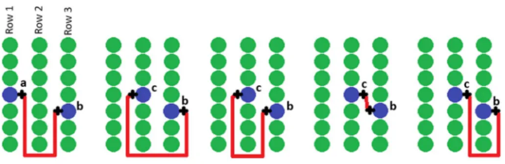
The method requires computation of a distance matrix. This matrix gives the dis-tance between each couple of PSSs. Disdis-tance must correspond to the shortest walking distance between the two PSSs. It must take into account the structure of the vineyard. Each PSS, located on one vine rows, can be accessed through two inter-rows (Fig. 1). As a result, each site appears twice in the distance matrix. If the sites are in the same inter-row, it corresponds to the classical Euclidian distance. If they belong to different inter-rows, the distance is computed considering that the practitioner has to get out the row, to reach the desired rows passing by all ends of intermediate rows and finally to reach the targeted sampling site (Fig. 1). As rows have two extremities, two different distances can be computed and the shortest one is kept.
Fig. 1 Distances across vineyards. The left illustrates how the vineyard structure affect the moving from point a to point b. The others illustrate the four different ways of going from point c to point b
Representative sampling based on auxiliary information
The same approach as Carrillo et al. (2016) was used to consider auxiliary data. It is sum-marised hereafter. The sampling approach aims at calibrating a linear regression which relates the yield (sampled) to auxiliary data. Carrillo et al. (2016) showed that yield com-ponents, especially berry weight, are linearly related to auxiliary data (NDVI) in non-irri-gated vineyard of south of France. The sampling approach aims at selecting sampling sites (SSs) representatively to build this linear model. This model is then used to estimate yield using all available high-resolution auxiliary data.
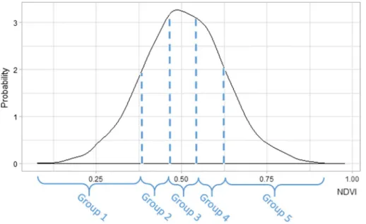
The approach proposed in this paper relies on the following principle. PSSs are split into N homogeneous groups (N corresponding to the number of samples) according to their auxiliary data values. Once groups are formed, one PSS from each group is selected in order to optimize the length of the route connecting all selected PSSs. This ensures the PSSs are representative of the field as selected points are spread across the auxiliary data distribution. Quantiles were used to make groups. Related work concluded that this approach was adapted to yield estimation (Oger et al. 2015). Quantiles method guarantees that the groups have the same number of PSS, K being the number of PSSs and N the num-ber of samples required, then each group has K
N elements (Fig. 2).
Route optimisation
The second step of the approach consists in selecting N sampling sites (one sampling site per group). These N sampling sites (SSs) must be all different and have to form the shortest possible sampling circuit. There are many possible choices to select these SSs and many ways to order them to form a circuit. It is therefore a highly combinatorial optimization problem. Constraint Programming is one of the programming paradigms
Fig. 2 NDVI values for groups with quantile approach and N = 5. Each group contains 20% (100/N) of PSS according to their NDVI values
able to deal with such problems. It aims at solving a problem expressed as a set of vari-ables and a set of constraints on these varivari-ables. Such a problem is called a Constraint Satisfaction Problem (CSP). A Constraint Solver is used to find a solution to the prob-lem that satisfies all the constraints. The efficiency of these solvers relies on the imple-mentation of many methods such as filtering, which allows a quick detection of combi-nations of values that do not lead to an optimal solution. The interest of constraint solvers lies in their ability to address many types of constraints. Without going into detail, let S = {1, … , K} be the set of PSSs and {Gi}i∈(1,…,N) the set of quantile groups
covering S, formed in the previous step from the auxiliary data. Since all these groups are disjoint subsets, {Gi}i∈(1,…,N) is a partition of S . Pi is defined as the selected site for
group Gi . Hence, set SSelected (the set sampling sites) will be equal to
{
Pi
}
i∈(1,…,N).
The first constraint imposes that all Pi must be different; because all quantile groups
are disjoint subsets, it is immediately satisfied in the case of the presented approach.
P0 represents the point of departure and arrival, it is a fixed parameter representing the
initial position of the practitioner. The length of the optimum route passing through all the Pi∈(0,…,N) must be minimum. This is a particular case of vehicle routing problem
(VRP) where the goal is not to find a Hamiltonian tour (visiting once every site) but a tour covering only a subset of sites. Recent work about the WeightedSubCircuit con-straint (Vismara and Briot 2018) has proposed a filtering algorithm that is well adapted to address this type of situation. All these constraints and variables constitute the con-straint satisfaction problem. An instance of this problem is built from each dataset and solved with the solver in order to get an ordered set of sites that form a sampling circuit. The program returns the list of sampling sites, the order in which they are visited and the associated walking distance.
Yield estimation
The aim is to estimate Y , the average yield of the field. For each selected sampling site s ( s ∈ SSelected ), GW(s) is the grape weight per vine value. A linear model linking the
aux-iliary data ( AD ) to GW is built from these sites (Eq. 1):
For a given site s , ̂GW(s) represents an estimate of GW(s) . The parameters a and b are obtained from a linear regression on the N sites selected by the sampling method.
With S = {1, … , K} being the full set of PSSs available, ̂YCS , the yield estimate with
Constrained Sampling (CS) approach, can be computed from the model using all these PSSs (Eq. 2):
Estimation error
Regardless of the method used, the estimation error is a deviation from the actual yield value ( Y ) and its estimation ( ̂Y ), expressed as a percentage (Eq. 3).
(1) ̂ GW(s) = a × AD(s) + b (2) ̂ YCS= means∈S(̂GW(s))
Reference methods
The method is compared to two references:
A conventional random sampling (RS) approach where the N sampling sites are randomly selected among all the PSSs. ̂YRS , the yield estimated with RS, is therefore directly calculated
from the mean of observed GW values. RS represents what is generally done in practice in terms of yield estimation.
The second approach is model sampling (MS) whose method principles have been described by (Carrillo et al. 2016). SSs are chosen according to NDVI values. One site is ran-domly selected for each of the N NDVI quantiles. MS uses a model based on the NDVI/yield relationship, as described in Eq. 1. Unlike constrained sampling method, the selection of SS does not consider their position on the plot.
To compare the length of the routes between the different methods, the optimal route between the selected sites was computed for both reference methods. This was done with the R TSP package (Hahsler and Hornik 2007).
Theoretical fields Methodology
Simulated data were used to study the properties and limitations of the approach. Theoretical fields are intended to compare CS to reference methods in a wide range of known situations. Each simulation aims at providing two variables for each theoretical field: auxiliary observa-tion (i.e. NDVI) and variable of interest (i.e. the yield), both spatially auto-correlated.
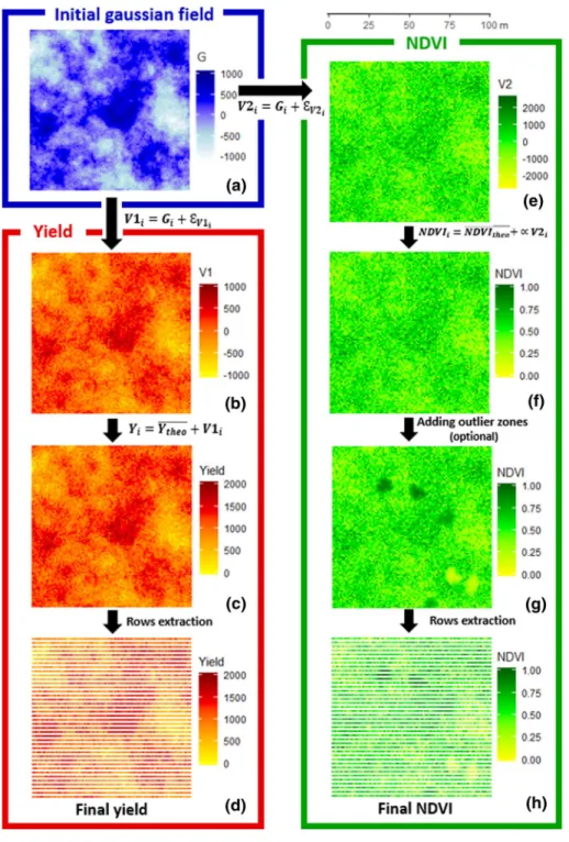
The simulation assumed that a main underlying phenomenon (i.e. environmental factors like soil, climate, elevation, etc.) drives the within field variability of the plant response. The simulation process therefore starts by generating a theoretical auto-correlated variable (noted
G ), representing the spatial variability of the underlying factor. G is simulated as a spatialized
Gaussian field with no nugget effect (Fig. 3a). Two new variables, respectively V1 (Fig. 3b) and V2 (Fig. 3e), were derived from G by adding a non-auto-correlated noise following a nor-mal centred distribution of respective variances 𝜎V1 and 𝜎V2 (Eqs. 5 and 6). V1 and V2 are
therefore intrinsically correlated with each other, the level of correlation depends on 𝜎V1 and
𝜎V2 . In the followings, V1 will be used for the variable of interest while V2 will be used for the
auxiliary variable. (3) Error(%) = ||| Y− ̂Y||| Y (4) ̂ YRS= means∈S Selected(GW(s)) (5) V1i= Gi+ 𝜀V1iwith 𝜀V1i∼ N ( 0, 𝜎2V1) (6) V2i= Gi+ 𝜀V2 i with 𝜀V2i ∼ N ( 0, 𝜎V22 )With Cor(V1, V2) 𝜖 [0,1]
Fig. 3 Workflow of the theoretical fields simulation process. a Variable G is generated as a fully spatial-ized Gaussian field. b Variable V1 derived from G by adding a random noise. c Yield variable derived from V1(linear transformation). d Final theoretical yield data after row extraction. e Variable V2 derived from G by adding a random noise. f Variable NDVI derived from V2 (linear transformation). g NDVI variable com-plemented with outlier zones. h Final NDVI data after row extraction
Four parameters were considered to vary across the theoretical dataset: (i) the distance of auto-correlation of G, V1 and V2, defined by the range of the semi-variogram of each variable; (ii) the ratio of nugget effect/sill of the V1 variable; (iii) the degree of correla-tion between V1 and V2 and (iv) the number of outliers on V2. These parameters fit the diversity of theoretical data by controlling the link between the two variables and their semi-variograms. Hereafter is described the process used to set up these parameters during the simulation process:
𝜎2
V1 , the variance of the noise added to V1 was chosen to obtain the expected nugget
effect/sill ratio on V1. G having no nugget effect, 𝜎2
V1 is therefore directly equal to the
nug-get effect of V1 . It can be directly deduced from the ratio and 𝜎2 s (Eq. 7):
𝜎2
V2 , the variance of the noise added to V2 was used to calibrate the degree of correlation
between V1 and V2 . This was deduced from the covariance and Pearson correlation formu-las (Eqs. 8 and 9).
Hence:
G , 𝜀V1 and 𝜀V2 being independent random variables, their covariance are equal to zero.
Finally:
With the Pearson correlation formula:
it results in:
And finally:
The variable of interest will be the yield and the auxiliary data, the NDVI. They were respectively derived from V1 and V2 by a linear change of scale ( 𝛼) to be centred around (7)
Ratio= nugget(Y)
sill(Y) = 𝜎2 V1 𝜎2 G ⇒ 𝜎2 V1= Ratio × 𝜎 2 G (8) Cov(V1, V2) = Cov(G+ 𝜀V1, G+ 𝜀V2)
Cov(V1, V2) = Cov(G, G) + Cov(G, 𝜀V1
)
+ Cov(G, 𝜀V2
)
+ Cov(𝜀V1, 𝜀V2)
Cov(V1, V2) = Cov(G, G) = Var(G) = 𝜎2G
Cor(V1, V2) =√ Cov(V1, V2) Var(V1) ×√Var(V2) (9) Cor(V1, V2) = 𝜎2 G √ 𝜎2 sG+ 𝜎 2 V1× √ 𝜎2 G+ 𝜎 2 V2 𝜎2 V2= ⎛ ⎜ ⎜ ⎜ ⎝ 𝜎2 G � 𝜎2 G+ 𝜎 2 V1× Cor(V1, V2) ⎞ ⎟ ⎟ ⎟ ⎠ 2 − 𝜎2G
the desired average yield ( Ytheo ) and the desired average NDVI ( NDVItheo ) with the
appro-priate dispersion (Eqs. 10 and 11) This transformation does not affect the correlation or any of the three other parameters. (Fig. 3c, f and Eqs. 10 and 11):
An optional step consists of adding outlier zones on the NDVI simulated maps. Outlier zones intended to represent abnormal phenomenon like weed patches (abnormally strong NDVI) or local diseased vines (abnormally low NDVI) who may locally alter the correla-tion between yield and NDVI.
The number of outlier zones will vary from 0 to 6 (Table 1). The Location of each outlier zones was randomly chosen. Their size varies from 10 to 30 pixels and all these pixels have the same NDVI value taken from [0.1,0.25] ∪ [0.75,0.9] . All these parameters are drawn randomly for each desired outlier zones. Pixels around the outlier zone were smoothed in order to simulate a short gradient with “normal” surrounding NDVI values (Fig. 3g). Introduction of outlier zones may lead to a slight decrease for the correlation parameter.
The final step consisted in extracting the values of both information (Yield and NDVI) corresponding to the rows of the vine. The rows take the values of the nearest pixel. (Fig. 3d and h).
Implementation
Theoretical fields were designed with an area of one hectare (100 m × 100 m) with a 2.5 m distance between rows which corresponds more or less to typical fields area and plantation density of 4000 vines/ha found in south of France. The resolution was 1 pixel/m2. For
theo-retical yield data, parameters of the simulation were defined so that average yield corre-sponds to common average yield of the region ( Ytheo− = 1000g∕vine) and Coefficient of
Vari-ation (CV) to previous works: CV = 30%; 𝜎2
G= (1000 × 0.3)
2 (Krstic et al. 1998, Dunn and
Martin 2000). For theoretical NDVI, the average value was set at NDVI−theo= 1∕2 , and the 𝛼
factor in Eq. 11 at 1
18𝜎G to ensure that all the NDVI values lay within the range of [0,1].
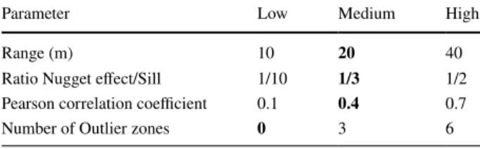
The choice of the different possible values for the four parameters (Table 1) was based on observations from literature in precision viticulture (Bramley et al. 2019, Bramley and Hamilton 2004, Hall et al. 2010, Li et al. 2017, Taylor et al. 2005, Tisseyre et al. 2008). For each parameter, three possible levels were defined (Table 1), encompassing a range of vari-ability allowing to account for the existing diversity in vineyard fields. Each parameter will
(10)
Yi= Ytheo+ V1i
(11)
NDVIi= NDVItheo+ V2i× 𝛼
Table 1 Values for theoretical field parameters
Default values are in bold font
Parameter Low Medium High
Range (m) 10 20 40
Ratio Nugget effect/Sill 1/10 1/3 1/2
Pearson correlation coefficient 0.1 0.4 0.7
vary individually by setting the others to their default values, indicated in bold in Table 1. This procedure will ensure to test the effect of each parameter on the sampling results.
Real data
Real fields used to test the method come from INRA Pech-Rouge (Narbonne, France). The experiment and the data base was detailed by Carrillo et al. (2016). It is briefly summarised hereafter. NDVI values from nine different vine fields were considered. All of them are non-irrigated and exposed to Mediterranean climate with precipitation occurring during spring with hot and dry summer. The characteristics of each plot are shown in Table 2. NDVI values were derived from a 1 m. resolution multi-spectral image taken the 31th of August 2008 by Avion Jaune (Montpellier, Hérault, France). The spectral regions captured in the images were: blue (445–520 nm) green (510–600 nm), red (632–695 nm) and near-infrared (757–853 nm). From these 1 m square image pixels, aggregation method described in (Acevedo-Opazo et al. 2008) was used to obtain 9 m square image pixels reducing the effect of canopy discontinuity and bare soil on measured values. NDVI was finally com-puted from processed images according to Rouse et al. (1973). Mechanical or chemical weeding was performed over the inter-row spacing; therefore, row cover crop did not affect much NDVI values.
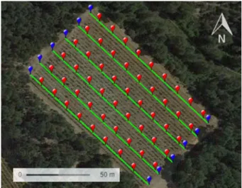
PSSs were selected regularly over the fields with measurement made on each node of a 15 m2 width sampling grid (Fig. 4). At each node, yield was measured on five consecutive
vines in the row and average yield was affected to the location corresponding to the central vine. The final data base was a set of 313 sites over the nine different fields. It is notewor-thy that, unlike simulated fields, the number of PSSs is reduced for real fields. Indeed, since it was not practically possible to measure the yield on each vine stock, the conse-quence is that the number of PSSs depends on the number of available measurement sites, therefore PSSs per site varied from 19 to 45. Each PSS was then characterized by a Grape Weight per vine value (GW) and a NDVI value.
For each field, the average of all available measured GW values was used to estimate the average yield of the field ( Y).
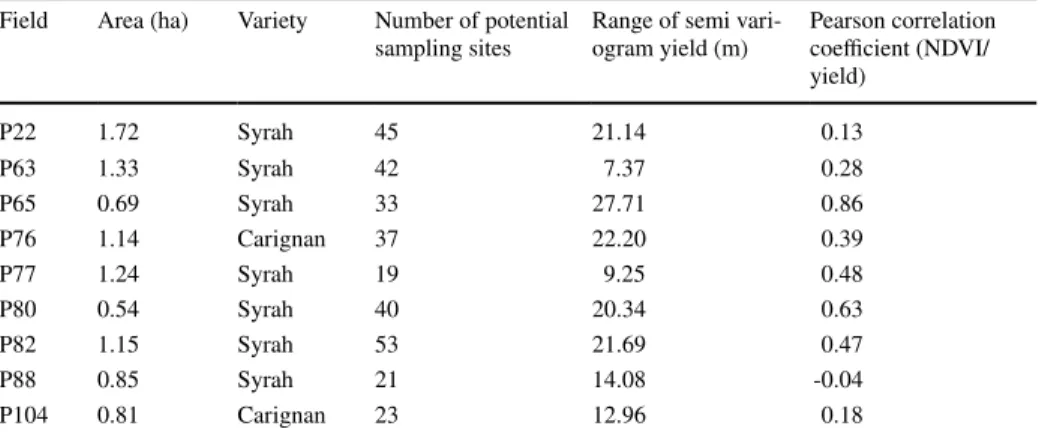
Table 2 Description of the experimental fields
Nugget effect could not be estimated because of the resolution of yield data Field Area (ha) Variety Number of potential
sampling sites Range of semi vari-ogram yield (m) Pearson correlation coefficient (NDVI/ yield) P22 1.72 Syrah 45 21.14 0.13 P63 1.33 Syrah 42 7.37 0.28 P65 0.69 Syrah 33 27.71 0.86 P76 1.14 Carignan 37 22.20 0.39 P77 1.24 Syrah 19 9.25 0.48 P80 0.54 Syrah 40 20.34 0.63 P82 1.15 Syrah 53 21.69 0.47 P88 0.85 Syrah 21 14.08 -0.04 P104 0.81 Carignan 23 12.96 0.18
Implementation
The core of the sampling approach was written in Java, the program used the Choco solver (Prud’homme et al. 2014). The calculations to obtain the distance matrix are made with Python. Theoretical fields, quantile classification according to their value for auxiliary data, estimation errors, and route distance were computed with R. Packages “gstats” and “sp” were used to generate Gaussian fields for the G variable.
As explained in the description of the constraints, the approach presented here takes into account the starting site of the practitioner to include it in the sampling circuit. Var-ying the starting site thus changes the result that will be obtained. In order to increase the number of situations tested for real data, this starting site is positioned on different ends of row across the vineyards. The approach was then applied to 86 different situa-tions instead of 9. Results for the different starting sites were averaged for each field. For theoretical data, thirty simulations per set of parameters are tested (270 in total). CS was applied once to each simulated plot. The starting site is located on one of the corners of the plot. The two outer rows on each side and the first three vines of each row cannot be selected as, in practice, they are subject to border effects. For both theoreti-cal and experimental data, RS and MS were applied 1000 times. These repetitions were possible as they rely on random or partially random selection of SSs. The following figures are based on the average of the results obtained on each field, the result of each field being the average across repetitions with different starting site.
Fig. 4 INRA Pech Rouge plot with row edges in blue and potential sampling sites in red (Color figure online)
Results and discussion
Sampling and vine diversity Number of sampling sites
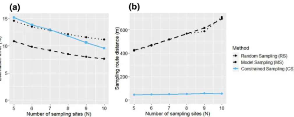
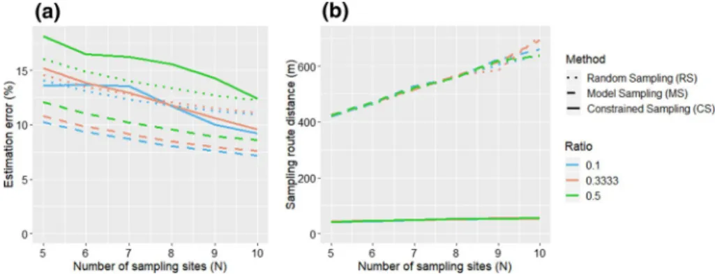
Figure 5 presents the results obtained for the three sampling approaches, constrained sampling (CS), model sampling (MS) and random sampling (RS) for simulated fields with parameters set at their default values (Table 1). The different sampling approaches were tested on each simulated plot with a number of measurement sites ranging from N = 5 to N = 10. Results represent the averages obtained with thirty simulated plots.
All the sampling methods follow the same trend with a decreasing error as the num-ber of sampled sites increases. This result is logical, and consistent with the literature. As Carrillo et al. (2016) have already shown, taking into account auxiliary data, MS approach slightly improves the quality of yield estimation compared to a RS (Fig. 5a). With default values, it seems that the MS approach proposed by Carrillo et al. (2016) gives the best results in terms of estimation error. CS and RS both present similar errors whatever the number of SSs. Observed errors with CS are higher than for MS (i.e. with-out constraints). This result may be logical considering that the addition of the con-straints may limit possibilities when choosing among the PSS.
Figure 5b clearly illustrates the gains brought by CS in terms of travel distance across the vineyard. Logically, the travelled distance within the plot increases linearly with N, the number of SSs. Travel distances with CS are at least 85% better than with other sampling methods. Distances are also less sensitive to the increase in the number of SSs with CS. This is explained by the gain brought by considering this criterion when selecting SSs. In view of these first results, CS offers a compromise between MS and distance criterion optimization, with a higher estimation error in favour of a significant reduction in distance.
With the hypothesis of a walking speed of 0.9 m/s and 60 s needed per SS, Table 3
shows that MS and CS perform better than RS. For a given amount of time, CS allows a higher number of observations to be made compared to other sampling approaches and therefore the lowest estimation error.
Fig. 5 Results for theoretical data with default parameters in function of the number of sampling sites; a estimation error, b sampling route distance
Impact of the semi‑variogram range
Figure 6 shows the estimation error and the distance results obtained with the 3 sampling approaches tested on theoretical fields with varying range (10 m, 20 m, 40 m) of semi-var-iograms. Varying the range does not affect significantly the estimation error in function of the number of SSs compared to previous results. MS still presents the best estimation error compared to CS and RS (Fig. 6a). For a range of 40 m, CS seems more erratic with the highest error for a low number of SSs (N > 8) and an estimation error which tends to the error observed with MS for a higher number of SSs (N > 8) As for estimation error, results of distances associated with RS and MS do not seem to be affected by the range parameter either (Fig. 6b). The increase in range is nevertheless associated with a slight increase in distance with CS.
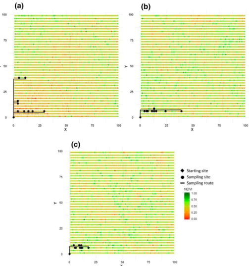
Figure 7 gives an illustration of the sampling route obtained with the method for plots with different ranges (10, 20 and 40 m).
The method always promotes the measurement sites in the immediate vicinity of the starting site (0.0 coordinates). This is expected as the method aims to minimize travel time. A robustness study (result not shown) showed that the results were similar regardless of the starting site, the method always promote measurement sites close to the starting point whatever the plot characteristics. Figure 7 shows that the average distance between sam-pling sites tends to increase with the plot range. On these plots, the maximum distance
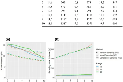
Table 3 Sampling time and estimation error for RS, MS and CS on simulated data
N Random sampling
(RS) Model sampling (MS) Constrained sam-pling (CS) Error (%) Time (s) Error (%) Time (s) Error (%) Time (s)
5 14,6 767 10,8 773 15,2 347 6 13,5 877 9,8 881 13,9 411 7 12,8 993 9,1 994 12,9 474 8 12,1 1111 8,5 1111 11,8 537 9 11,5 1192 7,9 1223 10,6 603 10 11,1 1387 7,6 1371 9,5 660
Fig. 6 Effect of the semi-variogram range on sampling strategies. a Estimation error & b sampling route distance
between sampling points corresponds approximately to the range of the plot; it is of 40 m, 30 m and 10 m respectively for plot range of 40 m, 20 m and 10 m. This result is expected since as the range increases, the distance to find a higher diversity of values also increases leading to longer sampling routes for larger ranges. This result is consistent with that of Fig. 6b.
One surprising aspect, at first glance, is the close proximity of the sampling points. This characteristic is related to the nugget effect, which introduces erratic variance and high variability over short distances. This erratic variance makes it possible to find a high var-iability of values in the immediate vicinity of the starting point and other measurement sites. The sampling method takes advantage of this variability to minimize travel time. It should be remembered that in these simulations, the nugget effect was defined according to literature figures in precision viticulture. It is rather high since it represents more than 30% of the plot variability.
Fig. 7 Illustration of sampling routes for N = 9 and three different ranges: a range = 40 m; b range = 20 m; c range = 10 m
A decrease in this nugget effect leads to longer sampling route. For example, if the nug-get effect is set to 0 (no erratic variability), then the sampling distance is longer since the distance needed to find representative values necessarily increases. Conversely in the case of no spatial autocorrelation, the method chooses contiguous independent measurement sites on a same row and the sampling distance is in this case very short (result no shown). Figure 7 therefore represents the result of optimal sampling that takes into account the combined effect of the nugget effect and the range considering realistic figures of spatial variability in viticulture.
Impact of the ratio nugget/sill
Figure 8 shows the impact of the ratio for the three sampling strategies. Whatever the sam-pling method and the number of samsam-pling points, an increasing ratio affect the estima-tion error (Fig. 8a). This result is logical since the increase in the ratio corresponds to an increase in the proportion of erratic (non-autocorrelated) variance in the total variance of the NDVI. Thus, sampling methods tend to select SSs whose NDVI value is not necessarily correlated to the expected yield value. Note that for a high ratio (ratio = 0.5), the estimation error with CS is more affected compared to other approaches. CS approach appears to be more sensitive to high ratio values. Indeed, the short-range variability introduced by higher erratic variance increase the chance to have sites in different quantile groups close to each other. The CS approach that minimizes the route from the starting site might select close SSs. Close SSs often provide redundant information, which leads to an increase in estima-tion error. On the other hand, the ratio does not seem to have any significant influence on the length of the sampling circuits (Fig. 8b).
Impact of the correlation level with auxiliary data
As expected, RS is not affected by a low level of correlation since SSs selection is not based on the NDVI data (Fig. 9a). This is not the case for MS and CS which both show lowest estimation errors when correlation between yield and NDVI is high while they show high estimation errors decreases when the correlation decreases. Since, MS and CS use the relationship between the two variables, it was expected that the quality of prediction decreases when this relationship is weakened. When the correlation is close to 0, MS tends
Fig. 8 Effect of the proportion of the ratio nugget/sill on sampling strategies. a Estimation error & b sam-pling route distance
to have the same results as RS while CS presents the worst estimation error. For the theo-retical dataset, a very low correlation corresponds to a strongly noisy NDVI (Eq. 9). The resulting short range erratic variability in NDVI could explain this result for CS. It follows the same phenomenon as already observed in the previous section for an increasing ratio. These results highlight the sensitivity of CS to noise in NDVI for the selection of SSs aim-ing at optimisaim-ing the distance. As for previous result, samplaim-ing distance does not seem much affected by the correlation, apart for CS for which it seems to slightly decrease with the correlation (Fig. 9b). This result supports the idea of a decreasing correlation allowing the CS approach to find SSs closer to each other.
Impact of outlier zones
The addition of local outlier (Fig. 10a) seems to slightly affect all methods, including the RS which should not be affected by changes in auxiliary data. The effect of outlier zones is still more important on the CS. It is difficult to draw conclusions as the effect is not propor-tional to the number of outlier zones. As it could be expected, the length of the sampling circuits is not affected by these local outlier zones (Fig. 10b).
Fig. 9 Effect of the correlation between NDVI and yield on sampling strategies. a Estimation error & b sampling route distance
Evaluation of sampling strategies on real data
Figure 11 shows the averaged result of the three sampling methods on real fields. The same logical decrease in error as the number of sampled sites increases is observed (Fig. 11a.) The irregularity of the curves associated with CS can be explained by a smaller number of experiments compared to results obtained with theoretical fields. With N = 6 put aside, CS estimation errors are just halfway between those of RS and MS. Considering the characteristic of real fields in terms of ratio and corre-lation between yield and NDVI (Table 1), these results are consistent with the results obtained on the simulated data. CS has been shown to be sensitive to the correlation between yield and NDVI and noise in NDVI values. The average correlation between yield and NDVI being quite large for real data (0.38 on average, Table 1) and NDVI values being smoothed, real fields present average characteristics close to the default values for theoretical fields. The reduction of erratic local variability in NDVI may have favoured results observed with real fields with CS. Figure 11b illustrates the gains in terms of travel distance across the vineyard when using CS compared to other sampling approaches. Distance is reduced by approx. 50% with CS compared to MS and RS. This result is again consistent with those observed with theoretical data. However, the gain here is much smaller than with theoretical data because of the lower number of PSSs available for real fields Considering the minimum distance between two PSSs is 15 m, the distance required to travel through the selected SS is necessarily higher for real fields because of the impossibility for the algorithm to find SSs closer than 15 m to each
Fig. 11 Results on real data. a Estimation error & b sampling route distance
Table 4 Sampling time and estimation error for RS, MS and CS on real data
N Random sampling
(RS) Model sampling (MS) Constrained sam-pling (CS) Error (%) Time (s) Error (%) Time (s) Error (%) Time (s)
5 24,4 755 19,2 761 22,7 506 6 22,3 855 17,9 863 27,2 611 7 20,5 949 15,5 961 18,7 696 8 18,9 1042 14,3 1052 15,8 797 9 17,8 1129 12,9 1144 13,9 892 10 16,8 1214 12 1225 14,7 981
other, while this was possible for theoretical fields. Overall, this method offers a good compromise between the quality of the estimate and the travel constraint on the plot.
Table 4 compares the performance of the different approaches on sampling time and estimation error for real data. Walking speed is set at 0.9 m/s and 60 s are required for each SS. As for simulated data, CS perform better (up to 30%) than other approaches for a given amount of time.
Further reflections
The method presented in this paper aims to select SSs accounting for variability high-lighted by auxiliary data and the practitioner constraints simultaneously. It is intended to be general enough to be applicable to various combinations of auxiliary data and variable of interest. This type of strategy could be applied to any type of crop where the travel route of operators is constrained by the organization of the crop (trellised structure). It may be necessary to keep in mind the assumptions on which the approach is based on: the fact that there is a correlation between the variable of interest and the auxiliary variable and the rel-evant auxiliary variable is available with a high spatial resolution.
The choice of the auxiliary variable depends on the variable of interest to be estimated and the pedo-climatic context of the crop. Returning to the application case presented in this paper, it is based on preliminary studies that indicate that the NDVI measured at verai-son was a relevant auxiliary variable to guide yield sampling in the specific context of non-irrigated Mediterranean vineyard. However, this same auxiliary variable may not be relevant in other soil and climatic contexts. As a result, the choice of the variables used requires prior knowledge and expertise for the correct implementation of the approach.
Overall, it seems that CS offers a strategy with relevant compromise between estimation error and sampling distance. It significantly improves the performance of the latter crite-rion for a small increase of the estimation error. For a given amount of time, CS presents better results than reference methods. For a given number of SSs, the gap for the average error between CS and MS, which also uses a model for estimating the variable of interest, could be explained by two points. First, the optimization of the distance tends to regroup the SSs around the starting point (Fig. 6), and it has been shown that this could be a dis-advantage when the auxiliary data is noisy, indeed in this case, CS favours the choice of different NDVI values very close to each other and not necessarily correlated with the vari-able of interest. Conversely, the other methods can be more representative as they are more likely to choose SSs anywhere over the plot. The second reason is that choosing points close to each other reduces the distance of the circuit but might increase the autocorrelation between measurements. Two close sites will provide more or less redundant information depending on the distance between them. It should be noted that on the plot, practition-ers generally rely on a random sampling limited to a fraction of the plot (often a pair of rows) as they cannot cover the whole field. The results obtained would then correspond to a degraded version of the random sampling due to the same auto-correlation problem.
A potential solution to minimize the gap between MS and CS would be to set a min-imum distance between two SSs. This minmin-imum distance could be derived from spatial auto-correlation of available auxiliary data or historical yield maps. This distance would be determined with the range of the experimental semi-variogram obtained with the auxiliary data. Depending on the value, this could make it possible to avoid or limit the autocorrela-tion issue between the SSs and to better results of CS for slightly longer sampling times. Another practical option when the auxiliary data is particularly noisy (ratio > 0.33), would
be to smooth the data using, for example, a moving window average. This was done on real fields of this study and gave particularly interesting results. The methodology proposed by Tisseyre et al. (2018) could be used to decide on the size of the smoothing window to be used according to the erratic variance that is to be eliminated. Each of these areas for consideration could improve the sampling method presented here with reduced estimation errors and more widely spaced measurement sites.
Other areas for improvement are possible, such as, for example, the ability to integrate multiple auxiliary data or to use more complex models.
Conclusion
The methodology presented in this paper describes a new approach, Constrained Sam-pling (CS), for yield samSam-pling in viticulture. The originality of the approach comes from the association of method from Carrillo et al. based on auxiliary data and optimisation algorithms to propose relevant sampling routes in term of estimation error and travelled distance. While the model sampling principle guides sampling points choice considering auxiliary information, optimisation through constraint programming ensures the relevancy of the chosen route in term of walking distance for the practitioner. CS appears however sensitive to unfavourable situations (low correlation, poor spatial structure, erratic variance of the auxiliary data) while other methods relying on random aspect may fare better. In favourable situations (good correlation between auxiliary data and yield and strong spatial structure), CS gives very good results. The estimation error is close to what is proposed by Carrillo et al. However, CS makes it possible to obtain much shorter sampling in distances and times. This saved time can then be used to increase the number of measurements and the reliability of the estimation.
Acknowledgements This work was supported by the French National Research Agency under the Invest-ments for the Future Program, referred as ANR-16-CONV-0004 (#Digitag).
References
Acevedo-Opazo, C., Tisseyre, B., Guillaume, S., & Ojeda, H. (2008). The potential of high spatial resolu-tion informaresolu-tion to define within-vineyard zones related to vine water status. Precision Agriculture, 9, 285–302.
Arnó, J., Martínez-Casasnovas, J. A., Uribeetxebarria, A., & Rosell-Polo, J. R. (2017). Comparing efficiency of different sampling schemes to estimate yield and quality parameters in fruit orchards. Advances in
Animal Biosciences, 8(2), 471–476.
Bramley, R. G. V., & Hamilton, R. P. (2004). Understanding variability in winegrape production systems. 1. Within vineyard variation in yield over several vintages. Australian Journal of Grape and Wine
Research, 10, 32–45.
Bramley, R. G. V., Ouzman, J., Trought, M. C. T., Neal, S. M., & Bennett, J. S. (2019). Spatio-temporal variability in vine vigour and yield in a Marlborough Sauvignon Blanc vineyard. Australian Journal of
Grape and Wine Research, 25(4), 430–438.
Briot, N., Bessiere, C., Tisseyre, B. & Vismara, P. (2015). Integration of Operational Constraints to Opti-mize Differential Harvest in Viticulture. In Proceed. 10th European conference on precision
agricul-ture (ECPA 2015), pp. 487–494.
Carrillo, E., Matese, A., Rousseau, J., & Tisseyre, B. (2016). Use of multi-spectral airborne imagery to improve yield sampling in viticulture. Precision Agriculture, 17(1), 74–92.
Cristofolini, F., & Gottardini, E. (2000). Concentration of airborne pollen of Vitisvinifera L. and yield fore-cast: A case study at S.Michele all’Adige, Trento, Italy. Aerobiologia, 16(1), 125–129.
Clingeleffer, P. R., Martin, S., Krstic, M., & Dunn, G. M. (2001). Crop development, crop estimation and
crop control to secure quality and production of major wine grape varieties. A national approach: Final report to grape and wine research & development corporation. Adelaide: Grape and Wine
Research & Development Corporation.
Dunn, G. M., & Martin, S. R. (2000). Spatial and temporal variation in vineyard yields. In Proceedings of
the fifth international symposium on cool climate viticulture & oenology. Precision management work-shop (pp. 1–4). Romsey: Cope Williams Winery.
Hall, A., Lamb, D. W., Holzapfel, B. P., & Louis, J. P. (2010). Within-season temporal variation in correla-tions between vineyard canopy and winegrape composition and yield. Precision Agriculture, 12(1), 103–117.
Hahsler, M., & Hornik, K. (2007). TSP—infrastructure for the traveling salesperson problem. Journal of
Statistical Software, 23(2), 1–21.
Krstic, M. P., Welsh, M. A., & Clingeleffe, P. R. (1998). Variation in chardonnay yield components between vineyards in a warm irrigated region. In R. J. Blair, A. N. Sas, P. F. Hayes, & P. B. Hoj (Eds.),
Preci-sion agriculture (pp. 269–270). Urrbrae, SA, Sydney Australia: AWRI.
Li, T., Hao, X., Kang, S., & Leng, D. (2017). Spatial variation of winegrape yield and berry composition and their relationships to spatiotemporal distribution of soil water content. American Journal of
Enol-ogy and Viticulture, 68(3), 369–377.
Oger, B., Vismara, P., & Tisseyre, B. (2015). Combining target sampling with route-optimization to opti-mise yield estimation in viticulture. In proceed. 12th European conference on precision agriculture
(ECPA 2019), pp. 487–494.
Prud’homme, C., Fages, J. G., & Lorca, X. (2014). Choco documentation. TASC, INRIA Rennes, LINA CNRS UMR 6241, COSLING S.A.S, https ://perso .ensta -paris .fr/~diam/jorla b/onlin e/choco /user_ guide -3.3.0.pdf.
Rouse, J. W. Jr., Haas, R. H., Schell, J. A., & Deering, D. W. (1973). Monitoring vegetation systems in the great plains with ERTS. In S. C. Freden, E. P. Mercanti, & M. A. Becker (Eds.), Proceedings of the
Third ERTS Symposium, NASA SP-351 1, pp. 309–317
Taylor J., Tisseyre B., Bramley R. & Reid A. (2005). A comparison of the spatial variability of vineyard yield in European and Australian production systems. In Proceed. 5th European conference on
preci-sion agriculture (ECPA 2005), pp. 907–914.
Tisseyre, B., Leroux, C., Pichon, L., Geraudie, V., & Sari, T. (2018). How to define the optimal grid size to map high resolution spatial data? Precision Agriculture, 19(5), 957–971.
Uribeetxebarria, A., Martínez-Casasnovas, J. A., Tisseyre, B., Guillaume, S., Escolà, A., Rosell-Polo, J. R., et al. (2019). Assessing ranked set sampling and ancillary data to improve fruit load estimates in peach orchards. Computers and Electronics in Agriculture, 164, 104931.
Vismara, P. & Briot, N. (2018). A circuit constraint for multiple tours problems. In proceed. 24th
interna-tional conference on principles and practice of constraint programming (CP 2018). Lecture Notes in Computer Science. (Vol. 11008, pp. 389–402).
Publisher’s Note Springer Nature remains neutral with regard to jurisdictional claims in published maps and institutional affiliations.