HAL Id: hal-01744505
https://hal.archives-ouvertes.fr/hal-01744505v3
Submitted on 28 Jun 2019
HAL is a multi-disciplinary open access
archive for the deposit and dissemination of
sci-entific research documents, whether they are
pub-lished or not. The documents may come from
teaching and research institutions in France or
abroad, or from public or private research centers.
L’archive ouverte pluridisciplinaire HAL, est
destinée au dépôt et à la diffusion de documents
scientifiques de niveau recherche, publiés ou non,
émanant des établissements d’enseignement et de
recherche français ou étrangers, des laboratoires
publics ou privés.
Tail expectile process and risk assessment
Abdelaati Daouia, Stephane Girard, Gilles Stupfler
To cite this version:
Abdelaati Daouia, Stephane Girard, Gilles Stupfler.
Tail expectile process and risk assessment.
Bernoulli, Bernoulli Society for Mathematical Statistics and Probability, 2020, 26 (1), pp.531-556.
�10.3150/19-BEJ1137�. �hal-01744505v3�
Tail expectile process and risk assessment
ABDELAATI DAOUIA1,* ST ´EPHANE GIRARD2,** and GILLES STUPFLER3,†
1
Toulouse School of Economics, University of Toulouse Capitole, France E-mail:*[email protected]
2
Universit´e Grenoble Alpes, INRIA, CNRS, Grenoble INP, LJK, 38000 Grenoble, France E-mail:**[email protected]
3School of Mathematical Sciences, University of Nottingham, Nottingham NG7 2RD, UK E-mail:†[email protected]
Expectiles define a least squares analogue of quantiles. They are determined by tail expectations rather than tail probabilities. For this reason and many other theoretical and practical merits, expectiles have recently received a lot of attention, especially in actuarial and financial risk man-agement. Their estimation, however, typically requires to consider non-explicit asymmetric least squares estimates rather than the traditional order statistics used for quantile estimation. This makes the study of the tail expectile process a lot harder than that of the standard tail quantile process. Under the challenging model of heavy-tailed distributions, we derive joint weighted Gaussian approximations of the tail empirical expectile and quantile processes. We then use this powerful result to introduce and study new estimators of extreme expectiles and the standard quantile-based expected shortfall, as well as a novel expectile-based form of expected shortfall. Our estimators are built on general weighted combinations of both top order statistics and asymmetric least squares estimates. Some numerical simulations and applications to actuarial and financial data are provided.
Keywords: Asymmetric least squares, Coherent risk measures, Expected shortfall, Expectile, Extrapolation, Extremes, Heavy tails, Tail index.
1. Introduction
Least asymmetrically weighted squares estimation, borrowed from the econometrics lit-erature, is one of the basic tools in statistical applications. This method often involves Newey and Powell’s [34] concept of expectiles, a least squares analogue of traditional quantiles. Given an order τ P p0, 1q, Koenker and Bassett [29] elaborated an absolute er-ror loss minimization to define the τ th quantile of the distribution of a random variable Y as the minimizer
qτP arg min θPR E tρ
τpY ´ θq ´ ρτpY qu ,
with equality if the distribution function of Y is increasing, where ρτpyq “ |τ ´ 1Ipy ď
0q| |y| and 1Ip¨q is the indicator function. This successfully extends the conventional def-inition of quantiles as left-continuous inverse functions. Newey and Powell [34] replaced
the absolute deviations in the asymmetric loss function ρτ with squared deviations to
obtain the τ th expectile of a random variable Y with finite first moment as ξτ “ arg min
θPR E tη
τpY ´ θq ´ ητpY qu , (1)
with ητpyq “ |τ ´ 1Ipy ď 0q| y2. Both quantiles and expectiles are M-quantiles as the
min-imizers of asymmetric convex loss functions (Breckling and Chambers [8]), but expectiles are determined by tail expectations rather than tail probabilities. Accordingly, expectiles have been receiving a lot of attention as risk measures in statistical finance and actuarial science since the pioneering paper of Kuan et al. [31]. As established very recently in this literature of risk management (see, for instance [6, 7, 13, 44]), expectiles are excellent alternatives to quantiles in different aspects relevant to this kind of applications. They depend on both the tail realizations and their probability, while quantiles only depend on the frequency of tail realizations and not on their values (Kuan et al. [31]). Expectiles, contrary to quantiles, thus allow to measure extreme risk based on both the frequency of tail losses and their severity. More generally, altering the shape of the upper or lower tail of Y does not change the quantiles of the other tail, but it does impact all the expectiles (Taylor [39]). This high sensitivity of expectiles to tail behavior allows for more prudent and reactive risk management. Another substantial difference is that expectiles rely on the distance to observations, whereas quantiles only use the information on whether an observation is below or above the predictor (Sobotka and Kneib [38]). Also, inference on expectiles is much easier than inference on quantiles (Abdous and Remillard [1]). Using expectiles avoids distributional assumptions (Taylor [39]) without recourse to regularity assumptions as can be seen by comparing, e.g., Holzmann and Klar [27] with Zwing-mann and HolzZwing-mann [45]. Most importantly, expectiles are the only M-quantiles that define a coherent risk measure in the sense of Artzner et al. [4] (see Bellini et al. [6]), and the only coherent risk measure that is elicitable (Ziegel [44]). Many other theoretical and numerical results motivate the adoption of expectiles in actuarial and financial risk management, including those of Ehm et al. [20] and Bellini and Di Bernardino [7].
Yet, tail expectile theory is, in comparison to tail quantile theory, relatively unexplored and still in full development. At the population level, only Bellini et al. [6], Mao et al. [32], Mao and Yang [33] and Bellini and Di Bernardino [7] have initiated the study of the connection between ξτ and qτ, as τ Ñ 1, when Y belongs to the domain of attraction of
a Generalized Extreme Value distribution. Also, for heavy-tailed distributions, Daouia et al. [13] have obtained an asymptotic expansion of ξτ{qτ with a precise quantification of
the remainder term. At the sample level, attention has been mainly restricted to ordinary expectiles of fixed asymmetry level τ staying away from the distribution tails; see, e.g., Holzmann and Klar [27] and Kr¨atschmer and Z¨ahle [30] for recent advanced theoretical developments. The extreme value analysis of asymmetric least squares estimators is a lot harder than for order statistics, mainly due to the absence of a closed form expression for expectiles. In an earlier paper, we partially solved this difficulty by proving the pointwise asymptotic normality of sample expectiles for ‘intermediate’ levels τ “ τn Ñ 1 such that
np1´τnq Ñ 8 as the sample size n Ñ 8; see Theorem 2 of Daouia et al. [13]. Such a result
expectiles. By contrast, Gaussian approximations of the tail empirical quantile process have been known for at least three decades; see, among others, Cs¨org˝o and Horv´ath [10] and Einmahl and Mason [21] as well as their more modern formulations in Drees [18] and Theorem 2.4.8 in de Haan and Ferreira [15]. These powerful asymptotic results, and their later generalizations, have been successfully used in the analysis of a number of complex statistical functionals, such as test statistics aimed at checking extreme value conditions (Dietrich et al. [17], Drees et al. [19], H¨usler and Li [28]), bias-corrected extreme value index estimators (de Haan et al. [16]) and estimators of extreme Wang distortion risk measures (El Methni and Stupfler [23,24]).
The present paper tries to fill this gap in the current understanding of sample inter-mediate expectiles, under Pareto-type models that accurately describe the tail structure of most actuarial and financial data [see, e.g., Embrechts et al. ([25], p.9) and Resnick ([35], p.1)]. In Section2, we show that the aforementioned convergence result on single intermediate sample expectiles can be generalized to the tail empirical expectile process. We first prove in Theorem 1 that the tail expectile process can be approximated by a sequence of Gaussian processes with drift and we derive its joint asymptotic behavior with the tail quantile process. Then, we analyze in Theorem 2 the difference between the tail empirical expectile process and its population counterpart. These two results constitute the major contribution of the paper; they open the door to the theoretical analysis of a wide range of functionals of the tail expectile process. Even more strongly, our joint weighted approximations of the tail empirical expectile and quantile processes make it possible to consider complex functionals of both processes.
We shall discuss below a number of applications of our main results. Section3applies the analysis of the tail expectile process in Theorem1 to extreme expectile estimation. We first construct a general class of weighted estimators for intermediate expectiles ξτn,
by combining nonparametric asymmetric least squares estimates with semiparametric quantile-based estimates. The latter involve the traditional Hill estimator of the tail in-dex (Hill [26]). Thanks to the joint convergence result on the tail expectile and quantile processes, in Theorem1, we derive the joint asymptotic normality of both empirical inter-mediate expectile and quantile estimators with Hill’s tail index estimator in Theorem3. Built on this theorem, we obtain the asymptotic normality of the generalized weighted ξτn estimators in Theorem 4. Based on the ideas of Daouia et al. [13], our weighted
intermediate expectile estimators are then extrapolated to the very extreme expectile levels that may approach one at an arbitrarily fast rate. The asymptotic properties of the extrapolated estimators are established in Theorem5.
Theorem2 is particularly important in tail risk estimation using Expected Shortfall (ES) measures. In Section4, we show first that the expectile-based form XTCEτ of ES
introduced by Taylor [39] is not a coherent risk measure. Instead, we define a coherent alternative form that we call XESτ. It is simply an average of tail expectiles, which is
in addition asymptotically equivalent to XTCEτ. Asymptotic connections of XESτ to
other tail quantities, such as high quantiles qτ and expectiles ξτ, are also provided in
Proposition 3 before moving on to the extreme value estimation problem. XESτ being
an average of tail expectiles, it is readily estimated at an intermediate level τ “ τn
XESτn can be unraveled thanks to Theorem 2. This intermediate estimator, like our
generalized expectile estimators, can then be extrapolated to the very far tails of the distribution of Y where few or no data lie. Financial institutions and insurance companies are typically interested in the extreme region τ “ τ1
n Ò 1 such that np1 ´ τn1q Ñ c ă 8,
as n Ñ 8 (see, for example, Cai et al. [9] and Daouia et al. [13]). In Theorems 7
and 8 we provide the asymptotic properties of the resulting extrapolated estimator, along with those of alternative plug-in estimators built on the asymptotic properties of XESτ in Proposition 3. We conclude this section by using XES estimators as the
basis for estimating the more traditional quantile-based ES (QES) itself. We derive three composite expectile-based estimators for QES, at extreme levels τ1
n, whose asymptotic
properties are established in Theorem9.
Section 5 contains a simulation study of the estimators introduced hereafter. Appli-cations to medical insurance data and financial returns data are presented in Section6. Section7concludes. The Supplementary Material document contains all proofs and aux-iliary results along with further simulation results.
2. Tail empirical expectile process
Suppose we observe independent copies tY1, . . . , Ynu of a random variable Y and denote
by Y1,n ď Y2,n ď ¨ ¨ ¨ ď Yn,n their nth order statistics. A high expectile ξτn of order
τn Ñ 1, as n Ñ 8, can be estimated by its empirical counterpart
r ξτn“ arg min uPR 1 n n ÿ i“1 rητnpYi´ uq ´ ητnpYiqs “ arg min uPR n ÿ i“1 ητnpYi´ uq. (2)
Here the expectile level τn approaches one at an ‘intermediate’ rate in the sense that
np1 ´ τnq Ñ 8 as n Ñ 8. By analogy to the well-known tail empirical quantile process
(see Definition 2.4.3 in de Haan and Ferreira [15])
p0, 1s Ñ R, s ÞÑpq1´ks{n :“ Yn´tksu,n,
where t¨u stands for the floor function and k “ kpnq Ñ 8 is a sequence of integers with k{n Ñ 0, we define the tail empirical expectile process to be the stochastic process
p0, 1s Ñ R, s ÞÑ rξ1´p1´τnqs.
Note that the tail quantile process is nothing but tqp1´p1´τnqsu0ăsď1 with τn “ 1 ´ k{n.
Our main objective in this section is to provide general asymptotic approximations of the tail expectile process by Gaussian processes, under the model assumption of heavy-tailed distributions. To this end, some preparatory remarks and work are necessary.
2.1. Statistical model and preliminary results
We focus on the maximum domain of attraction of Pareto-type distributions with tail index 0 ă γ ă 1. The survival functions of these heavy-tailed distributions can be
expressed as
F pyq :“ 1 ´ F pyq “ y´1{γLpyq, (3)
for y ą 0 large enough, where L is a slowly varying function at infinity, i.e., a positive function on the positive half-line satisfying Lptyq{Lptq Ñ 1 as t Ñ 8 for any y ą 0. Equivalently, by Corollary 1.2.10 in de Haan and Ferreira [15], the tail quantile function of Y , defined as U ptq :“ q1´t´1” infty P R | 1{F pyq ě tu, satisfies
lim tÑ8 U ptxq U ptq “ x γ for all x ą 0. (4)
The index γ tunes the tail heaviness of F : the larger the index, the heavier the right tail. Let Y´ “ minpY, 0q denote the negative part of Y . Then, together with condition
E|Y´| ă 8, the assumption γ ă 1 ensures that the first moment of Y exists, and hence
expectiles of Y are well-defined. It has also been found under (3) or equivalently (4) that ξτ
qτ
„ pγ´1´ 1q´γ as τ Ñ 1 (5)
(Bellini and Di Bernardino [7]). An asymptotic expansion of ξτ{qτ with a precise
quantifi-cation of the bias term is obtained in Corollary 1 of Daouia et al. [13] under the following standard second-order extreme value condition:
C2pγ, ρ, Aq For all x ą 0, lim tÑ8 1 Aptq „ U ptxq U ptq ´ x γ “ xγx ρ ´ 1 ρ
where ρ ď 0 and A is a function converging to 0 at infinity and having ultimately constant sign. Hereafter, pxρ´ 1q{ρ is to be read as log x when ρ “ 0.
The meaning and the rationale behind this second-order extension of the regular vari-ation condition (4) are extensively discussed in Beirlant et al. [5] and de Haan and Ferreira [15], along with abundant examples of commonly used continuous distributions satisfying C2pγ, ρ, Aq. The asymptotic expansion in Daouia et al. [13] can actually be
further strengthened to match our purposes, as follows.
Proposition 1. Assume that E|Y´| ă 8 and condition C2pγ, ρ, Aq holds, with 0 ă γ ă 1.
(i) We have, as τ Ñ 1, ξτ qτ “ pγ´1´ 1q´γ ˆ 1 ` γpγ ´1´ 1qγ qτ pEpY q ` op1qq ` ˆ pγ´1´ 1q´ρ 1 ´ γ ´ ρ ` pγ´1´ 1q´ρ´ 1 ρ ` op1q ˙ App1 ´ τ q´1 q ˙ .
(ii) Let τn Ñ 1 be such that np1 ´ τnq Ñ 8, and pick s P p0, 1s. Then ξ1´p1´τnqs ξτn “ s´γ ˆ 1 ` psγ´ 1qγpγ ´1´ 1qγ qτn pEpY q ` op1qq ` p1 ´ γqpγ ´1´ 1q´ρ 1 ´ γ ´ ρ ˆ s´ρ´ 1 ρ App1 ´ τnq ´1 qp1 ` op1qq ˙ .
Part (i) of this proposition relaxes the conditions in Corollary 1 of Daouia et al. [13] by removing their unnecessary assumption of strict monotonicity of F . Part (ii) gives the asymptotic expansion of intermediate expectiles akin to condition C2pγ, ρ, Aq for
intermediate quantiles, which also reads as q1´p1´τnqs qτn “ s´γ ˆ 1 `s ´ρ´ 1 ρ App1 ´ τnq ´1 qp1 ` op1qq ˙ .
2.2. Main results
It is well-known that, under condition C2pγ, ρ, Aq, the tail quantile process can be
approx-imated by a sequence of scaled Brownian motions with drift. Namely, one can construct a sequence Wn of standard Brownian motions and a suitable measurable function A0
such that sγ`1{2`ε ˇ ˇ ˇ ˇ ? k ˆ p q1´ks{n q1´k{n ´ s ´γ ˙ ´ γs´γ´1Wnpsq ´ ? kA0pn{kqs´γ s´ρ´ 1 ρ ˇ ˇ ˇ ˇ
converges in probability to 0 uniformly in s P p0, 1s for any sufficiently small ε ą 0 (see Theorem 2.4.8 in de Haan and Ferreira [15]). In addition to satisfying k Ñ 8 and k{n Ñ 0, the sequence of integers k “ kpnq should also satisfy?kA0pn{kq “ Op1q. The proof
of this approximation result reveals that it is valid for a suitable version of the quantile process, equal to the original one in distribution, on a rich enough probability space (potentially different from the original space on which the Yi’s are defined). We will work
in the sequel with this version of the quantile process and thus with the associated Yi’s.
Our weak convergence results in Sections3and4are of course unaffected by this choice. Full details of where this suitable choice of process has to be made can be found in the Supplementary Material document. Besides, the function A0 is actually asymptotically
equivalent to A, see Theorem 2.3.9 in de Haan and Ferreira [15]. We may therefore write:
p q1´p1´τnqs qτn “ s´γ ˜ 1 ` a 1 np1 ´ τnq γs´1Wnpsq ` s´ρ´ 1 ρ App1 ´ τnq ´1 q ` oP ˜ s´1{2´ε a np1 ´ τnq ¸¸ uniformly in s P p0, 1s, (6)
where we set k “ np1 ´ τnq, with τn Ñ 1 and np1 ´ τnq Ñ 8. As regards the tail
expectile process, it is known from Theorem 2 of Daouia et al. [13] that rξτn is, under
certain conditions, an asymptotically normal estimator of ξτn. Similarly to the uniform
approximation (6) of the tail quantile process, this result can be generalized to a uniform approximation of the tail expectile process s ÞÑ rξ1´p1´τnqs. This is the first main result of the paper.
Theorem 1. Suppose that E|Y´|2ă 8. Assume further that condition C2pγ, ρ, Aq holds,
with 0 ă γ ă 1{2. Let τn Ñ 1 be such that np1´τnq Ñ 8 and
a
np1 ´ τnqApp1´τnq´1q “
Op1q. Then there exists a sequence Wn of standard Brownian motions such that, for any
ε ą 0 sufficiently small, p q1´p1´τnqs qτn “ s´γ ˜ 1 `a 1 np1 ´ τnq γaγ´1´ 1 s´1W n ˆ s γ´1´ 1 ˙ `s ´ρ´ 1 ρ App1 ´ τnq ´1 q ` oP ˜ s´1{2´ε a np1 ´ τnq ¸¸ and ξr1´p1´τnqs ξτn “ s´γ ˆ 1 ` psγ´ 1qγpγ ´1´ 1qγ qτn pEpY q ` oPp1qq ` a 1 np1 ´ τnq γ2aγ´1´ 1 sγ´1 żs 0 Wnptq t´γ´1dt ` p1 ´ γqpγ ´1´ 1q´ρ 1 ´ γ ´ ρ ˆ s´ρ´ 1 ρ App1 ´ τnq ´1q ` oP ˜ s´1{2´ε a np1 ´ τnq ¸¸ uniformly in s P p0, 1s.
In the particular case s “ 1, Theorem1 entails a np1 ´ τnq ˜ r ξτn ξτn ´ 1 ¸ d ÝÑ γ2aγ´1´ 1 ż1 0 W ptq t´γ´1dt
where W denotes a standard Brownian motion. The right-hand side is a centered Gaus-sian random variable, whose variance is
γ3p1 ´ γq ż1 0 ż1 0 minps, tqpstq´γ´1ds dt “ 2γ 3 1 ´ 2γ.
We do therefore recover Theorem 2 of Daouia et al. [13], subject to the additional conditionanp1 ´ τnqApp1 ´ τnq´1q “ Op1q, but under the reduced moment condition
E|Y´|2 ă 8. Note that the bias condition
a
np1 ´ τnqApp1 ´ τnq´1q “ Op1q is also
re-quired in order to establish the desired approximation (6) for the tail quantile process. The latter approximation in the quantile case does not require, however, the extra as-sumptions that γ P p0, 1{2q and E|Y´|2ă 8. These conditions essentially guarantee that
the loss variable has a finite variance. This is not likely to be restrictive in practice, since in most studies on actuarial and financial data, the realized values of γ have been found to lie well below 1{2; see, e.g., the R package ‘CASdatasets’, Cai et al. [9], Daouia et al. [13] and the references therein.
Nevertheless, Theorem1does not compare directly the tail expectile process with its population counterpart s ÞÑ ξ1´p1´τnqs. Our second main result analyzes the discrepancy
between these two quantities. Such a comparison is particularly relevant when developing the asymptotic theory for integrals of the tail expectile process, as discussed below in Section 4. This result cannot be obtained as a direct corollary of Theorem 1, because Proposition1(ii) is not a uniform result.
Theorem 2. If the conditions of Theorem1hold with ρ ă 0, then there exists a sequence Wn of standard Brownian motions such that, for any ε ą 0 sufficiently small,
r ξ1´p1´τnqs ξ1´p1´τnqs “ 1 ` 1 a np1 ´ τnq γ2aγ´1´ 1 sγ´1 żs 0 Wnptq t´γ´1dt ` oP ˜ s´1{2´ε a np1 ´ τnq ¸ uniformly in s P p0, 1s.
Note that the Gaussian term appearing in Theorem 2 is exactly the same as in the approximation of the tail expectile process in Theorem1. Both theorems open the door to the analysis of the asymptotic properties of a vast array of functionals of the tail expectile and quantile processes. We discuss in the next sections particular examples where these results can be used to construct general weighted estimators of extreme expectiles and of an expectile-based analogue for the Expected Shortfall risk measure. Theorems1and2will be the key tools when it comes to unravel the asymptotic behavior of these estimators.
3. Extreme expectile estimation
In this section, we first return to intermediate expectile estimation by combining nonpara-metric asymnonpara-metric least squares estimates with semiparanonpara-metric quantile-based estimates to construct a more general class of estimators for high expectiles ξτn such that τn Ñ 1
and np1 ´ τnq Ñ 8 as n Ñ 8. Then we extrapolate the obtained estimators to the very
high expectile levels that may approach one at an arbitrarily fast rate.
Alternatively to the direct nonparametric estimator rξτn defined in (2), one may use
the asymptotic connection ξτn „ pγ
´1´ 1q´γq
quantile qτn, described in (5), to define the following indirect semiparametric estimator of ξτn: p ξτn :“ ` p γ´1 τn ´ 1 ˘´pγτn p qτn,
whereγpτn is a suitable estimator of the tail index γ. We will consider in the sequel the
Hill estimator (Hill [26])
p γτn“ 1 tnp1 ´ τnqu tnp1´τnqu ÿ i“1 log ˆ p q1´pi´1q{n p q1´tnp1´τnqu{n ˙ , (7)
which enjoys a high degree of popularity thanks to its simplicity and advantageous variance properties. Beirlant et al. [5] and de Haan and Ferreira [15] give an extensive overview of the asymptotic theory for this popular estimator.
More generally, one may also combine the two estimators pξτn and rξτn to define, for
β P R, the weighted estimator ξτ
npβq :“ β pξτn` p1 ´ βq rξτn.
The two special cases β “ 1 and β “ 0 correspond to the unique existing intermediate expectile estimators in the literature, namely, the estimators pξτn and rξτn first introduced
in Daouia et al. [13]. These were coined, respectively, “indirect estimator” and “direct estimator” to reflect the pure asymmetric least squares nature of the latter and the reliance of the former on quantiles. The limit distribution of their linear combination ξτ
npβq crucially relies on the asymptotic dependence structure between the tail expectile
and quantile processes established in Theorem 1, since ξτ
npβq is built on both of these
processes. More specifically, it relies on the following asymptotic dependence structure between the Hill estimatorpγτn and the intermediate sample quantile pqτn and expectile
r ξτn.
Theorem 3. Suppose that E|Y´|2ă 8. Assume further that condition C2pγ, ρ, Aq holds,
with 0 ă γ ă 1{2. Let τn Ñ 1 be such that np1 ´ τnq Ñ 8, and suppose that the bias
conditionanp1 ´ τnqApp1 ´ τnq´1q Ñ λ1P R is satisfied. Then,
a np1 ´ τnq ˜ p γτn´ γ, p qτn qτn ´ 1,ξrτn ξτn ´ 1 ¸ d ÝÑ N pm, Vq where m is the 1 ˆ 3 vector
m:“ ˆ λ1 1 ´ ρ, 0, 0 ˙ , and V is the 3 ˆ 3 symmetric matrix with entries
Vp1, 1q “ γ2, Vp1, 2q “ 0, Vp1, 3q “ γ 3 p1 ´ γq2pγ ´1 ´ 1qγ, Vp2, 2q “ γ2, Vp2, 3q “ γ2 ˆ pγ´1´ 1qγ 1 ´ γ ´ 1 ˙ , Vp3, 3q “ 2γ 3 1 ´ 2γ.
Based on the joint asymptotic normality in Theorem3, we obtain the following limit distribution of the weighted estimator ξτ
npβq.
Theorem 4. Suppose that the conditions of Theorem3 hold with the additional bias conditionanp1 ´ τnq{qτnÑ λ2P R. Then, for any β P R,
a np1 ´ τnq ˜ ξτnpβq ξτn ´ 1 ¸ d ÝÑ β`b ` rp1 ´ γq´1´ logpγ´1´ 1qsΨ ` Θ˘` p1 ´ βqΞ where the bias component b is b “ λ1b1` λ2b2 with
b1 “ p1 ´ γq´1´ logpγ´1´ 1q 1 ´ ρ ´ pγ´1´ 1q´ρ 1 ´ γ ´ ρ ´ pγ´1´ 1q´ρ´ 1 ρ , b2 “ ´γpγ´1´ 1qγEpY q,
and pΨ, Θ, Ξq is a trivariate Gaussian centered random vector with covariance matrix V as in Theorem3.
Remark 1. The same second-order conditions involving the auxiliary function A in Theorems 3and 4 are also required to derive the marginal asymptotic normality of the conventional Hill estimatorpγτn, with asymptotic bias λ1{p1 ´ ρq and asymptotic variance
γ2[see Theorem 3.2.5 in de Haan and Ferreira ([15], p.74)]. Theorem4features, however, a further bias condition involving the quantile function q; this was to be expected in view of Proposition1(ii), of which a consequence is that the remainder term in the approximation ξ1´p1´τnqs{ξτn« s
´γ depends on both A and q.
Remark 2. When β “ 1, we recover the convergence of the ‘indirect’ estimator pξτn
obtained in Corollary 2 of Daouia et al. [13]. When β “ 0, we get the convergence of the ‘direct’ estimator rξτn stated in Theorem 2 of [13].
The use of the weighted estimator ξτnpβq is, by construction, most appropriate when it comes to deal with intermediate expectile levels τ “ τnÑ 1 such that np1 ´ τnq Ñ 8.
In the very far tails where the expectile level τ “ τ1
n Ñ 1 is such that np1 ´ τn1q Ñ
c P r0, 8q, this estimator becomes unstable and inconsistent due to data sparsity. To estimate an extreme expectile ξτ1
n, Daouia et al. [13] propose to extrapolate any consistent
intermediate expectile estimator, say qξτn, to the very high level τ
1
n by considering the
generic class of estimators q ξ‹ τ1 n:“ ˆ 1 ´ τ1 n 1 ´ τn ˙´qγn q ξτn,
where qγn is a suitable estimator of γ. Here, we choose to use the general weighted
in-termediate estimator ξτnpβq in conjunction with the Hill estimator pγτn to define the
following class of extreme expectile estimators: ξ‹τ1 npβq :“ ˆ 1 ´ τ1 n 1 ´ τn ˙´pγτn ξτnpβq. (8)
The two special cases β “ 1 and β “ 0 correspond to the unique existing extreme expectile estimators in the literature, namely, the extrapolated indirect and direct ex-pectile estimators suggested in Daouia et al. [13]. The next theorem gives the asymptotic behavior of the generalized extreme expectile estimators ξ‹τ1
npβq.
Theorem 5. Suppose that the conditions of Theorem 4hold. Assume also that ρ ă 0 and np1 ´ τ1
nq Ñ c ă 8 with
a
np1 ´ τnq{ logrp1 ´ τnq{p1 ´ τn1qs Ñ 8. Then, for any
β P R, a np1 ´ τnq logrp1 ´ τnq{p1 ´ τn1qs ˜ ξ‹τ1 npβq ξτ1 n ´ 1 ¸ d ÝÑ N ˆ λ1 1 ´ ρ, γ 2 ˙ .
One can observe that the limiting distribution of ξ‹τ1
npβq is controlled by the asymptotic
distribution of pγτn. In particular, in the cases β “ 1 and β “ 0, we exactly recover
Corollaries 3 and 4 of Daouia et al. [13] on the convergence of the extrapolated indirect and direct expectile estimators.
4. Estimation of tail Expected Shortfall
4.1. Background
The risk of a financial position Y is usually summarized by a risk measure %pY q, where % is a mapping from a space of random variables to the real line. Value at Risk (VaR) is arguably the most common risk measure used in practice. It is given at probability level τ P p0, 1q by the τ -quantile VaRτpY q :“ qτ. Hereafter, we adopt the convention that Y
is a real-valued random variable whose values are the negative of financial returns. The right-tail of the distribution of Y , for levels τ close to one, then corresponds to extreme losses.
One of the main criticisms of VaRτ is that it does not account for the size of losses
beyond the level τ , since it only depends on the frequency of tail losses and not on their values (Dan´ıelsson et al. [11]). Furthermore, VaRτ fails to be subadditive, since the
inequality VaRτpY1` Y2q ď VaRτpY1q ` VaRτpY2q does not hold in general (Acerbi [2]).
It is therefore not a coherent risk measure in the sense of Artzner et al. [4], which is problematic in risk management.
An important alternative to VaRτ is Expected Shortfall at level τ . This risk measure
is defined as (Acerbi [2]) QESτ:“ 1 1 ´ τ ż1 τ qtdt. (9)
When Y is continuous, QESτ is identical to the Conditional Value at Risk (Rockafellar and Uryasev [36, 37]), known also as Tail Conditional Expectation (TCE), defined as QTCEτ :“ ErY |Y ą qτs. Both QESτ and QTCEτ can then be interpreted as the average
a coherent risk measure but QTCEτ does not in general (see Wirch and Hardy [43] and Acerbi and Tasche [3]).
4.2. Expectile-based Expected Shortfall
Motivated by the merits and good properties of expectiles, Taylor [39] has introduced an expectile-based form of Expected Shortfall (ES) as the expectation XTCEτ :“ ErY |Y ą
ξτs of exceedances beyond the τ th expectile ξτ of the distribution of Y . This
expectile-based TCE was actually implemented by Taylor [39] only as an intermediate instrument for the ultimate interest in estimating the conventional quantile-based form QTCEτ, or equivalently, the coherent version QESτ under the continuity assumption on Y . Al-though the interpretability of XTCEτ is straightforward, its coherence as a proper risk
measure has been an open question so far. This is now elucidated below in Proposition2, showing the failure of XTCEτ to fulfill the coherence property in general. It would then
be awkward to use this non-coherent measure as the basis for estimating the coherent quantile-based version QESτ. Instead, by analogy to QESτ itself, we propose to use the new expectile-based form of ES
XESτ:“ 1 1 ´ τ ż1 τ ξtdt, (10)
obtained by substituting the expectile ξt in place of the quantile qt in the standard
form (9) of ES. It turns out that, in contrast to XTCEτ, the new risk measure XESτ is
coherent in general.
Proposition 2. For all τ ě 1{2,
(i) XESτ induces a coherent risk measure;
(ii) XTCEτ is neither monotonic nor subadditive in general, and hence does not induce
a coherent risk measure.
The coherence property of XESτ, contrary to that of QESτ, is actually a
straightfor-ward consequence of the coherence of the expectile-based risk measure ξτ, for τ ě 1{2.
Next, we show under the model assumption (3) that XESτ is asymptotically equivalent
to XTCEτ as τ Ñ 1, and hence inherits its direct meaning as the conditional expectation
ErY |Y ą ξτs for all τ large enough.
Proposition 3. Assume that E|Y´| ă 8 and that Y has a Pareto-type distribution (3)
with tail index 0 ă γ ă 1. Then XESτ QESτ „ξτ qτ „ XTCEτ QTCEτ and XESτ ξτ „ 1 1 ´ γ „ XTCEτ ξτ as τ Ñ 1.
Propositions 2 and 3 then afford arguments to justify that the new form XESτ of
measure, but also as an intermediate tool for estimating the classical quantile-based version QESτ. Indeed, XESτ is coherent and keeps the intuitive meaning of XTCEτ as
a conditional expectation when τ Ñ 1, since XESτ „ XTCEτ. Most importantly, XESτ
may be adopted as a reasonable alternative to QESτitself. As is the case in the duality (5) between the expectile ξτ and the VaR qτ, the choice in any risk analysis between the
expectile-based form XESτ and its quantile-based analogue QESτ will then depend on
the value at hand of γ ž 12. More precisely, the quantity XESτ will be more (respectively,
less) extreme than QESτ and hence more (respectively, less) pessimistic or conservative in practice, for all τ large enough, if γ ą 12 (respectively, γ ă12).
The connections in Proposition3 are very useful when it comes to interpreting and proposing estimators for XESτ. Also, by considering the second-order regular variation
condition C2pγ, ρ, Aq, one may establish a precise control of the remainder term which
arises in the asymptotic equivalent XESτ{ξτ„ p1 ´ γq´1.
Proposition 4. Assume that E|Y´| ă 8. Assume further that condition C2pγ, ρ, Aq
holds, with 0 ă γ ă 1. Then, as τ Ñ 1, XESτ ξτ “ 1 1 ´ γ ˆ 1 ´ γ 2 pγ´1´ 1qγ qτ pEpY q ` op1qq ` 1 ´ γ p1 ´ γ ´ ρq2pγ ´1 ´ 1q´ρApp1 ´ τ q´1 qp1 ` op1qq ˙ .
This result will prove instrumental when examining the asymptotic properties of our tail expectile-based ES estimators in the next section.
4.3. Estimation and asymptotics
Propositions1(i) and4 indicate that the expectile-based ES satisfies a regular variation property in the same way as quantiles and expectiles do. To estimate an extreme value XESτ1
n, where τ
1
n Ñ 1 and np1 ´ τn1q Ñ c ă 8, we may therefore start by estimating
XESτn, with τn being an intermediate level, before extrapolating this estimator to the
far tail using an estimator of the tail index γ. A natural estimator of XESτn is its direct
empirical counterpart: Ć XESτn :“ 1 1 ´ τn ż1 τn r ξtdt,
obtained simply by replacing ξtin (10) with its sample version rξtdescribed in (2). Since
this estimator is a linear functional of the tail empirical expectile process, Theorem2 is more adapted than Theorem1 for the analysis of its asymptotic distribution.
Theorem 6. Under the conditions of Theorem 2, a np1 ´ τnq ˜ Ć XESτn XESτn ´ 1 ¸ d ÝÑ N ˆ 0,2γ 3 p1 ´ γqp3 ´ 4γq p1 ´ 2γq3 ˙ .
On the basis of Proposition1(ii) and then Proposition 3, we have for τn ă τn1 Ñ 1 that XESτ1 n XESτn „ξτ 1 n ξτn «ˆ 1 ´ τ 1 n 1 ´ τn ˙´γ . Therefore, to estimate XESτ1
n at an arbitrary extreme level τ
1
n, we replace γ by the Hill
estimatorpγτn and XESτn at an intermediate level τn by the estimator ĆXESτn to get
Ć XES‹τ1 n:“ ˆ 1 ´ τ1 n 1 ´ τn ˙´pγτn Ć XESτn. (11)
The next result analyzes the convergence of this Weissman-type estimator. Theorem 7. Assume that the conditions of Theorem 5hold. Then
a np1 ´ τnq logrp1 ´ τnq{p1 ´ τn1qs ˜ Ć XES‹τ1 n XESτ1 n ´ 1 ¸ d ÝÑ N ˆ λ1 1 ´ ρ, γ 2 ˙ .
One can also design alternative options for estimating XESτ1
n by using the
asymp-totic connections in Proposition 3. For example, the asymptotic equivalence XESτ1 n „
p1 ´ γq´1ξτ1
n, established therein, suggests that XESτn1 can be estimated consistently by
substituting the tail quantities γ and ξτ1
nwith their consistent estimatorspγτnand ξ
‹ τ1
npβq
described in (7) and (8), respectively. This yields the extrapolated estimator XES‹τ1
npβq :“ r1 ´pγτns
´1ξ‹ τ1
npβq, (12)
with a weight β P R, whose asymptotic normality is established in the following. Theorem 8. Assume that the conditions of Theorem 5hold. Then, for any β P R,
a np1 ´ τnq logrp1 ´ τnq{p1 ´ τn1qs ˜ XES‹τ1 npβq XESτ1 n ´ 1 ¸ d ÝÑ N ˆ λ1 1 ´ ρ, γ 2 ˙ .
Theorems 7 and8 are, like Theorem5, derived by noticing that, on the one hand, the asymptotic behaviors of ĆXES‹τ1
n and ξ
‹ τ1
npβq are controlled by the asymptotic behavior
of tp1 ´ τ1
nq{p1 ´ τnqu´p
γτn, which is itself governed by that of
p
γτn only. This is why, in
Theorems 7 and 8, the asymptotic distributions of ĆXES‹τ1
n and XES
‹ τ1
npβq coincide. On
the other hand, the nonrandom remainder term coming from the use of Proposition 3
can be controlled thanks to Proposition4.
4.4. Extreme level selection
A major practical question that remains to be addressed is the choice of the extreme level τ1
n in the tail risk measure XESτ1
n. Since XESτn1 „ ErY |Y ą ξτn1s, this problem translates
into choosing ξτ1 n itself.
When moving from the conventional VaR qpn, for a pre-specified tail probability
pn Ñ 1 with np1 ´ pnq Ñ c ă 8, to the expectile ξτ1
n, Bellini and Di Bernardino [7]
have suggested to pick out τ1
n so that ξτ1
n ” qpn. The expectile ξτn1 then inherits the same
intuitive probabilistic interpretation as the quantile qpn while keeping its coherence. This
idea was, however, implemented for a normally distributed Y . Instead, Daouia et al. [13] have suggested to estimate nonparametrically the level τ1
n that satisfies ξτ1
n“ qpn,
with-out recourse to any a priori distributional specification apart from the standard assump-tion (3) of heavy tails. By taking the derivative with respect to θ in the L2 criterion (1) and setting it to zero, we get
τ “ E t|Y ´ ξτ|1IpY ď ξτqu E |Y ´ ξτ|
for all τ P p0, 1q. The extreme expectile level τ1
nppnq :“ τn1 such that ξτ1 n ” qpn then satisfies 1 ´ τ1 nppnq “ E t|Y ´ q pn| 1I pY ą qpnqu E |Y ´ qpn| . Under the model assumption of Pareto-type tails (3), it turns out that
1 ´ τ1
nppnq „ p1 ´ pnq
γ
1 ´ γ as n Ñ 8.
The proof of this result can be found in Daouia et al. ([13], Proposition 3). Built on the Hill estimatorpγτn of γ, we can then define a natural estimator of τ
1 nppnq as p τ1 nppnq :“ 1 ´ p1 ´ pnq p γτn 1 ´γpτn . (13)
By substituting this estimated value in place of τ1
n” τn1ppnq in the extrapolated
estima-tors ĆXES‹τ1
n and XES
‹ τ1
npβq described in (11) and (12), we obtain composite estimators
that estimate XESτ1
nppnq„ QESpn, by Proposition 3. The convergence results in
Theo-rems7and8of the extrapolated estimators ĆXES‹τ1
nand XES
‹ τ1
npβq still hold true for their
composite versions as estimators of QESpn, with the same technical conditions.
Theorem 9. Suppose the conditions of Theorem5 hold with pn in place of τn1. Then,
for any β P R, a np1 ´ τnq logrp1 ´ τnq{p1 ´ pnqs ˜ Ć XES‹ p τ1 nppnq QESpn ´ 1 ¸ d ÝÑ N ˆ λ1 1 ´ ρ, γ 2 ˙ , and a np1 ´ τnq logrp1 ´ τnq{p1 ´ pnqs ˜ XES‹ p τ1 nppnqpβq QESpn ´ 1 ¸ d ÝÑ N ˆ λ1 1 ´ ρ, γ 2 ˙ .
5. Numerical simulations
In order to illustrate the behavior of the presented estimation procedures of the two expected shortfall forms XESτ1
nand QESpn, we consider the Student t-distribution with
degree of freedom 1{γ, the Fr´echet distribution F pxq “ e´x´1{γ, x ą 0, and the Pareto
distribution F pxq “ 1 ´ x´1{γ, x ą 1. The finite-sample performance of the
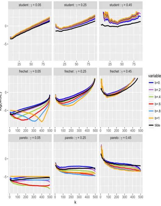
differ-ent estimators is evaluated through their relative Mean-Squared Error (MSE) and bias, computed over 200 replications. The accuracy of the weighted estimators is investigated for various values of the weight β P t0, 0.2, 0.4, 0.6, 0.8, 1u. All the experiments have sam-ple size n “ 500 and tail index γ P t0.05, 0.25, 0.45u. In our simulations we used the extreme levels τ1
n“ pn “ 1 ´n1 and the intermediate level τn“ 1 ´kn, where the integer
k can be viewed as the effective sample size for tail extrapolation.
5.1. Estimates of XES
τ1 nWe evaluated the finite-sample performance of ĆXES‹τ1
n and XES
‹ τ1
npβq, described in (11)
and (12), as estimators of XESτ1
n, for the different chosen scenarios and values of β.
Figures1and2give, respectively, the MSE (on a logarithmic scale) and bias estimates of XES‹τ1
npβq{XESτ 1
n, as functions of the sample fraction k (each curve corresponds to a
value of β as indicated by the colour-scheme). The Monte-Carlo estimates obtained for Ć
XES‹τ1
n{XESτn1 are superimposed in black curves. In the case of Student distribution (top
panels), the latter estimates perform clearly better in terms of both MSE and bias, for all values of γ. In the case of Fr´echet distribution (panels in the middle), it may be seen that the orange curves pβ “ 1q behave quite well in terms of MSE and bias, for the three values of γ. In the case of Pareto distribution (bottom panels), it may be seen from left to right that the green pβ “ 0.4q, blue pβ “ 0.8q and orange pβ “ 1q curves are superior, respectively, for γ “ 0.05, 0.25, 0.45.
To summarize, ĆXES‹τ1
n is the winner in the case of the real-valued Student
distribu-tion, while XES‹τ1
npβq appears to be the most efficient in the case of the non-negative
Fr´echet and Pareto distributions. The best choice of the weight β in the case of Fr´echet distribution is globally β “ 1. By contrast, the best choice of β in the case of Pareto distribution seems to increase with γ.
5.2. Estimates of QES
pnWe have also undertaken simulation experiments to evaluate the finite-sample perfor-mance of the composite versions ĆXES‹
p τ1 nppnqand XES ‹ p τ1
nppnqpβq studied in Theorem9, with
p τ1
nppnq being described in (13). These composite expectile-based estimators estimate the
same conventional expected shortfall QESp
n as the direct quantile-based estimator
z QES‹p n:“ ˆ 1 ´ pn 1 ´ τn ˙´γpτn 1 tnp1 ´ τnqu tnp1´τnqu ÿ i“1 Yn´i`1,n (14)
pareto : γ = 0.05 pareto : γ = 0.25 pareto : γ = 0.45 frechet : γ = 0.05 frechet : γ = 0.25 frechet : γ = 0.45 student : γ = 0.05 student : γ = 0.25 student : γ = 0.45
0 100 200 300 400 500 0 100 200 300 400 500 0 100 200 300 400 500 0 100 200 300 400 500 0 100 200 300 400 500 0 100 200 300 400 500 25 50 75 25 50 75 25 50 75 -5 0 -5 0 -5 0 k lo g (MSE) variable b=0 b=.2 b=.4 b=.6 b=.8 b=1 tilde
Figure 1. MSE estimates (in log scale) of ĆXES‹τ1
n{XESτn1 (black) and XES
‹ τ1
npβq{XESτn1
(colour-scheme), against k, for Student (top), Fr´echet (middle) and Pareto (bottom) distributions, with γ “ 0.05
pareto : γ = 0.05 pareto : γ = 0.25 pareto : γ = 0.45 frechet : γ = 0.05 frechet : γ = 0.25 frechet : γ = 0.45 student : γ = 0.05 student : γ = 0.25 student : γ = 0.45
0 100 200 300 400 500 0 100 200 300 400 500 0 100 200 300 400 500 0 100 200 300 400 500 0 100 200 300 400 500 0 100 200 300 400 500 25 50 75 25 50 75 25 50 75 -0.5 0.0 0.5 1.0 1.5 2.0 -0.5 0.0 0.5 1.0 1.5 2.0 -0.5 0.0 0.5 1.0 1.5 2.0 k Bi a s variable b=0 b=.2 b=.4 b=.6 b=.8 b=1 tilde
Figure 2. Bias estimates of ĆXES‹τ1
n{XESτn1 (black) and XES
‹ τ1
introduced by El Methni et al. [22]. To save space, all figures illustrating our simulation results here are deferred to the Supplementary Material document. In Supplement A, we arrive at the following tentative conclusions:
• In the case of the (real-valued) Student distribution, the best estimator seems to be ĆXES‹
p τ1
nppnq;
• In the cases of Fr´echet and Pareto distributions (both positive), the best estimators seem to be XES‹ p τ1 nppnqpβ “ 1q and/or zQES ‹ pn.
6. Applications
6.1. Application to medical insurance data
The Society of Actuaries (SOA) group Medical Insurance large claims database contains 75,789 claim amounts exceeding 25,000 USD, collected over the year 1991 from 26 in-surers. The full database which records about 3 million claims over the period 1991-92 is available at http://www.soa.org. The scatterplot and histogram of the 1991 log-claim amounts, displayed in Figure3(a), exhibit a considerable right-skewness. Beirlant et al. ([5], p.123) have argued that the underlying distribution is heavy-tailed with a γ estimate around 0.35. A traditional instrument to assess the magnitude of future unex-pected higher claim amounts is the exunex-pected shortfall QESpndescribed in (9). Insurance companies typically are interested in an extremely low exceedance probability of the or-der of 1{n, say, 1 ´ pn“ 1{100,000 for the sample size n “ 75,789. This corresponds to
rare events that happen on average only once in 100,000 cases.
In this situation of non-negative data with heavy right tail, our experience with sim-ulated data indicates that XES‹
p τ1
nppnqpβ “ 1q and zQES ‹
pn provide the best extrapolated
pointwise estimates of the extreme value QESpn in terms of MSE and bias. As such, these are the estimates we adopt here. For the sake of simplicity, XES‹
p τ1
nppnqpβ “ 1q will
be denoted in the sequel by XES‹
p τ1
nppnq.
The path of the composite expectile-based estimator XES‹
p τ1
nppnq against the sample
fraction k is shown in Figure3(b) as rainbow curve, for the selected range of intermediate values of k “ 10, 11, . . . , 700. The effect of the Hill estimate pγ1´k{n on XES
‹ p τ1
nppnq is
highlighted by a colour-scheme, ranging from dark red (lowpγ1´k{n) to dark violet (high p
γ1´k{n). This γ estimate seems to mainly vary within the interval r0.35, 0.36s, which corresponds to the stable (blue-green) part of the plot over k P r150, 500s. The curve k ÞÑ XES‹
p τ1
nppnq exceeds overall the sample maximum Yn,n “ 4.51 million (indicated by
the horizontal pink dashed line). To select a reasonable pointwise estimate, we applied a simple automatic data-driven device similar to that of El Methni et al. [23]. This consists first in computing the standard deviations of XES‹
p τ1
nppnq over a moving window large
enough to cover 20% of the possible values of k in the selected range 10 ď k ď 700. Then one selects the first window over which the standard deviation has a local minimum, and is less than the average standard deviation across all windows. The desired sample
fraction is finally defined as the value of k for which XES‹
p τ1
nppnq is the median estimate
within this window. The resulting estimate XES‹
p τ1
nppnq“ 6.42 million is obtained for the
value k “ 222 in the window r119, 259s.
The path of the direct quantile-based estimator zQES‹pn against k is graphed in the same figure as dashed black curve. It is very similar to that of XES‹
p τ1
nppnq. The pointwise
estimate zQES‹pn“ 6.37 million is indicated by the minimal standard deviation achieved at k “ 222 over the window r119, 259s. By Theorem9 we have
? k logrk{np1 ´ pnqs ˜ XES‹ p τ1 nppnq QESpn ´ 1 ¸ d ÝÑ N ˆ λ1 1 ´ ρ, γ 2 ˙ .
Under the bias condition λ1 “ 0 in Theorem 3, the asymptotic bias reduces to zero.
With this condition, the (symmetric) expectile-based asymptotic confidence interval with confidence level 100ϑ% has the form CIϑpkq “ XES
‹ p τ1
nppnqˆ I, where I stands for the
interval I :“ „ 1 ˘ zp1`ϑq{2 log ˆ k np1 ´ pnq ˙ p γ1´k{n ? k , (15)
with zp1`ϑq{2 being the p1 ` ϑq{2´quantile of the standard Gaussian distribution. The confidence interval derived from the asymptotic normality of zQES‹pn in [22] can be ex-pressed as xCIϑpkq “ zQES
‹ pnˆ I.
The two asymptotic 95% confidence intervals CI0.95pkq and xCI0.95pkq are superimposed
in Figure3(b) as well, respectively, in dotted blue and solid grey lines. Clearly, they point towards similar conclusions. In particular, the stable parts of their lower boundaries (around k P r100, 500s) remain quite conservative as they are very close to the maximum recorded claim amount.
Finally, we would like to comment on the estimator pτ1
nppnq of the extreme expectile
level τ1
nppnq which ensures that XES ‹ p τ1
nppnq estimates XESτn1ppnq „ QESpn. The plot of
p τ1
nppnq versus k is graphed in Figure3(c) as rainbow curve, and the corresponding optimal
pointwise estimate is indicated by the horizontal dashed black line. This selected optimal levelτp1
nppnq “ 0.9999941 is higher than the pre-specified relative frequency pn“ 0.99999
indicated by the horizontal dashed pink line. This is actually in line with our theoretical findings in Proposition3 that lead in conjunction with (5) to
XESpn
QESpn „ ξpn
qpn
„ pγ´1´ 1q´γ as pnÑ 1.
Since γ ă 1{2, it follows that XESpn is less extreme than QESpn„ XESτn1ppnq, for all pn
large enough. Therefore pnă τn1ppnq by monotonicity of τ ÞÑ XESτ, which follows from
the fact that XESτ“ p1 ´ τ q´1
ş1
τξtdt, where the expectile function t ÞÑ ξtis continuous
6.2. Application to financial data
In this section, we apply our method to estimate the ES for three large US financial institutions. We consider the same investment banks as in the study of Cai et al. [9], namely Goldman Sachs, Morgan Stanley and T. Rowe Price. All of these banks had a market capitalization greater than 5 billion USD at the end of June 2007. The dataset consists of the negative log-returns pYiq on their equity prices at a weekly frequency
during 10 years from July 3rd, 2000, to June 30th, 2010. The choice of the frequency of data and time horizon follows the same set-up as in Cai et al. [9] and Daouia et al. [13]. Our theorems being derived under the assumption that the data Y1, . . . , Yn
are independent and identically distributed, we use here weekly rather than daily loss returns to reduce substantially the potential serial dependence. This results in the sample size n “ 522. We use our composite expectile-based method to estimate the standard quantile-based expected shortfall QESp
n, or equivalently the expectile-based expected
shortfall XESτ1
nppnq, with an extreme relative frequency pn“ 1 ´
1
n that corresponds to
a once-per-decade rare event.
In this situation of real-valued profit-loss distributions, our experience with simulated data indicates that the composite estimator ĆXES‹
p τ1
nppnqprovides the best QESpnestimates
in terms of MSE and bias. In the estimation, we employ the intermediate sequence τn “ 1 ´ k{n as before, for the selected range of values k “ 1, . . . , 80. The confidence
interval with confidence level 100ϑ% derived from the asymptotic normality of ĆXES‹
p τ1
nppnq,
in Theorem9, has the form ĂCIϑpkq “ ĆXES ‹ p τ1
nppnqˆ I, where I is described in (15). For our
comparison purposes, we use as a benchmark the direct quantile-based estimator zQES‹p
n
of El Methni et al. [22], along with the corresponding asymptotic confidence interval x
CIϑpkq.
For each bank, we superimpose in Figure4 the plots of the two competing estimates Ć XES‹ p τ1 nppnq and zQES ‹
pn against k, as rainbow and dashed black curves respectively, along
with their associated 95% confidence intervals ĂCI0.95pkq in dotted blue lines and xCI0.95pkq
in solid grey lines. The effect of the Hill estimatepγ1´k{n on ĆXES‹
p τ1
nppnqis highlighted by
a colour-scheme, ranging from dark red (lowpγ1´k{n) to dark violet (highpγ1´k{n). We have already provided Monte Carlo evidence that the composite expectile-based estimator ĆXES‹
p τ1
nppnq is efficient relative to the pure quantile-based estimator zQES
‹ pn.
Its superiority in terms of plots’ stability, including confidence intervals, can clearly be visualized in Figure 4 for the three banks. The final ES levels based on the selection criterion of Section 6.1, computed over a moving window covering 20% of the possible values of k, are reported in Table1, along with the asymptotic 95% confidence intervals of the ES. Based on the ĆXES‹
p τ1
nppnq estimates (in the second column), the ES levels for
Goldman Sachs and T. Rowe Price seem to be close (around ´38% to ´44%), whereas the ES level for Morgan Stanley is almost twice higher (around ´81%). It is worth noticing that the difference between the ĆXES‹
p τ1
nppnqlevels for Goldman Sachs and T. Rowe Price is
very close to the difference between their respective maxima Yn,n. The zQES ‹
(in the fourth column) point towards slightly more pessimistic risk measures for the three banks. Bank XESĆ ‹ p τ1 nppnq CIĂ0.95 QESz ‹ pn CIx0.95 Yn,n Goldman Sachs 0.445 (0.194, 0.620) 0.495 (0.226, 0.680) 0.365 Morgan Stanley 0.817 (0.384, 1.305) 0.883 (0.366, 1.478) 0.904 T. Rowe Price 0.386 (0.213, 0.511) 0.407 (0.216, 0.548) 0.305
Table 1. ES levels of the three investment banks, with the 95% confidence intervals and the sample
maxima. Results based on weekly loss returns, with n “ 522 and pn“ 1 ´n1.
Our two applications with real data seem to indicate that the more accurate composite expectile-based estimates tend to be less (respectively, more) conservative than the pure quantile-based estimates zQES‹pn in the case of real-valued profit-loss (respectively, non-negative loss) distributions.
7. Concluding remarks
Originally introduced in Newey and Powell [34], expectiles have found recently an increas-ing usage in finance and actuarial science as alternative instruments of risk protection to quantiles. Their estimation via the method of asymmetric least squares is still in full de-velopment in the areas of risk management and extreme value statistics. Our general joint theory for tail empirical expectile and quantile processes opens new horizons for a wide variety of tail risk estimation problems. This is illustrated through a fruitful estimation of Expected Shortfall (ES), based on general weighted combinations of both top order statistics and high expectiles. Interestingly, pure asymmetric least squares estimators are particularly advantageous in the case of real-valued profit-loss distributions.
In our motivating application we focus on both quantile and expectile-based forms of ES, but our weighted approximation theorems can be applied to other complex risk functionals of both expectile and quantile processes. This includes the wider class of co-herent spectral risk measures (Acerbi [2]), but also the very recent concept of extremiles (Daouia et al. [12]). The latter concept defines a new least squares analogue of quantiles, which is motivated via several angles and includes the family of expected minima and expected maxima. Its characterization as weighted average of all quantiles, as well as its specific merits and strengths, raise the question of extending this concept by replacing quantiles with expectiles. The class of Wang [41] distortion risk measures with concave distortion functions is another concrete example of genuine interest for future research. The formulation and estimation of extreme versions of these coherent risk measures, tack-led for instance in Vandewalle and Beirlant [40] and El Methni and Stupfler [23,24], can also be adapted and extended by substituting expectiles in place of quantiles and apply-ing our general theory. Yet another example of generalized quantile-based risk measures where similar considerations may be relevant is the family of so-called Lp-quantile risk
Supplementary Material
The supplement to this article contains simulation results along with technical lemmas and the proofs of all our theoretical results.
Acknowledgements
The authors would like to thank the referees, the Associate Editor and the Editor-in-Chief for their valuable suggestions which have improved the presentation of the paper. The research of A. Daouia was supported by the Toulouse School of Economics Individual Research Fund (IRF/Daouia-20125). S. Girard gratefully acknowledges the support of the Chair Stress Test, Risk Management and Financial Steering, led by the French Ecole Polytechnique and its Foundation and sponsored by BNP Paribas, as well as the support of the French National Research Agency in the framework of the Investissements d’Avenir program (ANR-15-IDEX-02).
References
[1] Abdous, B. and Remillard, B. (1995). Relating quantiles and expectiles under weighted-symmetry, Ann. Inst. Statist. Math., 47, 371–384.
[2] Acerbi, C. (2002). Spectral measures of risk: A coherent representation of subjective risk aversion, Journal of Banking and Finance, 26, 1505–1518.
[3] Acerbi, C. and Tasche, D. (2002). On the coherence of expected shortfall, Journal of Banking and Finance, 26, 1487–1503.
[4] Artzner, P., Delbaen, F., Eber, J.-M. and Heath, D. (1999). Coherent Measures of Risk, Math. Finance, 9, 203–228.
[5] Beirlant, J., Goegebeur, Y., Segers, J. and Teugels, J. (2004). Statistics of Extremes: Theory and Applications, Wiley.
[6] Bellini, F., Klar, B., M¨uller, A. and Gianina, E.R. (2014). Generalized quantiles as risk measures, Insurance Math. Econom., 54, 41–48.
[7] Bellini, F. and Di Bernardino, E. (2017). Risk management with expectiles, The European Journal of Finance, 23, 487–506.
[8] Breckling, J. and Chambers, R. (1988). M-quantiles, Biometrika, 75, 761–772. [9] Cai, J.J., Einmahl, J.H.J., de Haan, L. and Zhou, C. (2015). Estimation of the
marginal expected shortfall: the mean when a related variable is extreme, J. R. Stat. Soc. Ser. B, 77, 417–442.
[10] Cs¨org˝o, M. and Horv´ath, L. (1987). Approximation of intermediate quantile pro-cesses, J. Multivariate Anal., 21, 250–262.
[11] Dan´ıelsson, J., Embrechts, P., Goodhart, C., Keating, C., Muennich, F., Renault, O. and Shin, H.S. (2001). An Academic Response to Basel II. Special paper no. 130, Financial Markets Group, London School of Economics.
[12] Daouia, A., Gijbels, I. and Stupfler, G. (2018). Extremiles: A new perspective on asymmetric least squares, J. Amer. Statist. Assoc., to appear. Available at
https://www.tandfonline.com/doi/full/10.1080/01621459.2018.1498348. [13] Daouia, A., Girard, S. and Stupfler, G. (2018). Estimation of tail risk based on
extreme expectiles, J. R. Stat. Soc. Ser. B, 80, 263–292.
[14] Daouia, A., Girard, S. and Stupfler, G. (2019). Extreme M-quantiles as risk mea-sures: From L1to Lp optimization, Bernoulli, 25, 264–309.
[15] de Haan, L. and Ferreira, A. (2006). Extreme Value Theory: An Introduction, Springer-Verlag, New York.
[16] de Haan, L., Mercadier, C. and Zhou, C. (2016). Adapting extreme value statistics to financial time series: dealing with bias and serial dependence, Finance Stoch., 20, 321–354.
[17] Dietrich, D., de Haan, L. and H¨usler, J. (2002). Testing extreme value conditions, Extremes, 5, 71–85.
[18] Drees, H. (1998). On smooth statistical tail functionals, Scand. J. Stat., 25, 187–210. [19] Drees, H., de Haan, L. and Li, D. (2006). Approximations to the tail empirical distribution function with application to testing extreme value conditions, J. Statist. Plann. Inference, 136, 3498–3538.
[20] Ehm, W., Gneiting, T., Jordan, A. and Kr¨uger, F. (2016). Of quantiles and expec-tiles: consistent scoring functions, Choquet representations, and forecast rankings (with discussion), J. R. Stat. Soc. Ser. B, 78, 505–562.
[21] Einmahl, J.H.J. and Mason, D.M. (1988). Strong limit theorems for weighted quan-tile processes, Ann. Probab., 16, 1623–1643.
[22] El Methni, J., Gardes, L. and Girard, S. (2014). Nonparametric estimation of ex-treme risks from conditional heavy-tailed distributions, Scand. J. Stat., 41, 988– 1012.
[23] El Methni, J. and Stupfler, G. (2017). Extreme versions of Wang risk measures and their estimation for heavy-tailed distributions, Statist. Sinica, 27, 907–930.
[24] El Methni, J. and Stupfler, G. (2018). Improved estimators of extreme Wang distor-tion risk measures for very heavy-tailed distribudistor-tions, Econometrics and Statistics, 6, 129–148.
[25] Embrechts, P., Kl¨uppelberg, C. and Mikosch, T. (1997). Modelling Extremal Events for Insurance and Finance, Springer.
[26] Hill, B.M. (1975). A simple general approach to inference about the tail of a distri-bution, Ann. Statist., 3, 1163–1174.
[27] Holzmann, H. and Klar, B. (2016). Expectile asymptotics, Electron. J. Stat., 10, 2355–2371.
[28] H¨usler, J. and Li, D. (2006). On testing extreme value conditions, Extremes, 9, 69–86.
[29] Koenker, R. and Bassett, G.S. (1978). Regression quantiles, Econometrica, 46, 33– 50.
[30] Kr¨atschmer, V. and Z¨ahle, H. (2017). Statistical inference for expectile-based risk measures, Scand. J. Stat., 44, 425–454.
the Conditional Autoregressive Expectile models, J. Econometrics, 2, 261–270. [32] Mao, T., Ng, K. and Hu, T. (2015). Asymptotic expansions of generalized quantiles
and expectiles for extreme risks, Probab. Engrg. Inform. Sci., 29, 309–327.
[33] Mao, T. and Yang, F. (2015). Risk concentration based on expectiles for extreme risks under FGM copula, Insurance Math. Econom., 64, 429–439.
[34] Newey, W.K. and Powell, J.L. (1987). Asymmetric least squares estimation and testing, Econometrica, 55, 819–847.
[35] Resnick, S. (2007). Heavy-Tail Phenomena: Probabilistic and Statistical Modeling, Springer.
[36] Rockafellar, R.T. and Uryasev, S. (2000). Optimization of Conditional Value-at-Risk, Journal of Risk, 2, 21–42.
[37] Rockafellar, R.T. and Uryasev, S. (2002). Conditional Value-at-Risk for General Loss Distributions, Journal of Banking and Finance, 26, 1443–1471.
[38] Sobotka, F. and Kneib, T. (2012). Geoadditive expectile regression, Comput. Statist. Data Anal., 56, 755–767.
[39] Taylor, J. (2008). Estimating value at risk and expected shortfall using expectiles, Journal of Financial Econometrics, 6, 231–252.
[40] Vandewalle, B. and Beirlant, J. (2006). On univariate extreme value statistics and the estimation of reinsurance premiums, Insurance Math. Econom., 38, 441–459. [41] Wang, S.S. (1996). Premium calculation by transforming the layer premium density,
ASTIN Bull., 26, 71–92.
[42] Weissman, I. (1978). Estimation of parameters and large quantiles based on the k largest observations, J. Amer. Statist. Assoc., 73, 812–815.
[43] Wirch, J.L. and Hardy, M.R. (1999). A synthesis of risk measures for capital ade-quacy, Insurance Math. Econom., 25, 337–347.
[44] Ziegel, J.F. (2016). Coherence and elicitability, Math. Finance, 26, 901–918. [45] Zwingmann, T. and Holzmann, H. (2016). Asymptotics for the expected shortfall,
0 5000 10000 15000 10 12 14 log(Claims) co u n t 0 4000 8000 12000 16000 Count
(a) Histogram
2500000 5000000 7500000 10000000 12500000 0 200 400 600 Sample fraction k Pa th s 0.30 0.33 0.36 0.39 γ^1−k n(b) ES plots
0.999990 0.999992 0.999994 0.999996 0 200 400 600 Sample fraction k τ^n 0.30 0.33 0.36 0.39 γ^1−k n(c) Expectile level
Figure 3. (a) Scatterplot and histogram of the log-claim amounts. (b) The ES plots k ÞÑ XES‹
p τ1
nppnqpβ “
1q as rainbow curve, and k ÞÑ zQES‹pn in dashed black, along with the constant sample maximum Yn,n
in horizontal dashed pink. The confidence intervals CI0.95pkq in dotted blue lines and xCI0.95pkq in solid
grey lines. (c) The plot of k ÞÑ τp
1
nppnq as rainbow curve, along with the selected optimal pointwise
0.3 0.6 0.9 1.2 0 20 40 60 80 k ES 0.30 0.35 0.40 0.45 0.50 γ^1−k n
(a) Goldman Sachs
0.5 1.0 1.5 0 20 40 60 80 k ES 0.6 0.8 1.0 γ^1−k n
(b) Morgan Stanley
0.25 0.50 0.75 1.00 1.25 0 20 40 60 80 k ES 0.2 0.3 0.4 0.5 γ^1−k n(c) T. Rowe Price
Figure 4. Results based on weekly loss returns of the three investment banks: (a) Goldman Sachs, (b)
Morgan Stanley, and (c) T. Rowe Price, with n “ 522 and pn“ 1 ´ 1{n. The estimates ĆXES‹
p τ1
nppnq as
rainbow curve and zQES‹pn as dashed black curve, along with the asymptotic 95% confidence intervals
Ă
CI0.95pkq in dotted blue lines and xCI0.95pkq in solid grey lines. The sample maximum Yn,n indicated in