The coupled development of terrain and vegetation : the case of semiarid grasslands

The Coupled Development of Terrain and

Vegetation: The Case of Semiarid Grasslands

by

Javier Homero Flores Cervantes

C.E., Universidad Nacional Aut6noma de Mexico (2001) S.M., Massachusetts Institute of Technology (2004)

Submitted to the Department of Civil and Environmental Engineering in partial fulfillment of the requirements for the degree of

Doctor of Philosophy

at the

Massachusetts Institute of Technology

February 2010

ARCHNES

MASSACHUSETS INSTrfUTE OF TECHNOLOGY

MAR 2

3

2010

LIBRARIES

@

2010 Massachusetts Institute of Technology. All rights reserved.

Author...

...

...

Department of Civil and Environmental Engineering

January 8, 2010

Certified by...

Pr ssor

Rafael L. Bras

of Civil and Environmental Engineering

Thesis Supervisor

A ccepted by ...

...

Daniele Veneziano

Chairman, Departmental Committee for Graduate Students

The Coupled Development of Terrain and Vegetation: The

Case of Semiarid Grasslands

by

Javier Homero Flores Cervantes

Submitted to the Department of Civil and Environmental Engineering on January 8, 2010, in partial fulfillment of the

requirements for the degree of

Doctor of Philosophy in the Field of Hydrology

ABSTRACT

The distribution of vegetation in semiarid landscapes organizes as a function of mois-ture availability, which is often mediated by the form of the land surface. Simultane-ously the processes that shape the land surface are influenced by vegetation, mainly because vegetation reduces fluvial erosion. This thesis presents the study of the bidi-rectional interaction between vegetation and the land form in semiarid grasslands.

Remotely sensed data and digital elevation maps are used to infer the relationship between vegetation cover and topographic attributes at two field sites in the semiarid southwestern United States. A positive relationship between drainage area (a proxy for water accumulation) and vegetation, and a negative relationship between solar radiation incidence and vegetation, are identified.

The Channel-Hillslope Integrated Landscape Development (CHILD) model is mod-ified to include a detailed representation of soil moisture dynamics, vegetation dy-namics, seasonality of the solar forcing and rainfall, spatial variability of the incidence angle of solar radiation, and intrastorm variability of rainfall intensity. The soil mois-ture and vegetation dynamics components of the model are calibrated and compared to observations from a small catchment in southeastern Arizona. The representation of the evolution in time of evapotranspiration, soil moisture and above ground vege-tation, and of the spatial distribution of vegetation with the model, are satisfactory. CHILD was used to simulate the evolution of the landscape under bare surface, uniform and stationary vegetation, and dynamic vegetation conditions to evaluate the effects of a dynamic vegetation cover in ten thousand years. In these simulations the emergence of bedrock outcrops that lead to significant runoff, erosion, and the accumulation of sediments and moisture downstream of the bedrock-regolith interface, had the most significant impact in the landscape. Erosion was greatest in the bedrock outcrops, and bands of sediment and moisture accumulation in their downstream ends lead to the development of bands of vegetation that augmented the accumulation of sediment and runoff infiltration.

Thesis Supervisor: Rafael L. Bras

Acknowledgments

I gratefully acknowledge the support provided by the Department of Civil and En-vironmental Engineering through the Schoettler Fellowship, the support provided by the U. S. Army Research Office (agreement DAAD 19-01-1-0513), and NSF for the support provided through a biocomplexity grant (EAR 0642550).

I thank David Goodrich, Lainie Levick, Chandra Holifield and Susan Moran from the Southwest Watershed Research Center, for the LIDAR derived DEM, Landsat TM images and soil and hydrometeorological data provided for the grassland site in southeastern Arizona; and The Sevilleta Long Term Ecological Research (LTER) Program, for the DEM and grass biomass maps of the central New Mexico site made available on the internet.

I am grateful to my advisor for giving me the opportunity to work with him and be here surrounded by so many opportunities, brilliant and hardworking people, and resources. I feel privileged to be here.

I am grateful to my thesis committee members other than Rafael: Elfatih Eltahir, Erkan Istanbulluoglu, Ignacio Rodriguez Iturbe, and Kelin Whipple. Some of them came from distant cities to the thesis committee meetings, or constantly provided me with input by e-mail, to help me guide my research. Thank you.

I also wish to thank all the help from professors and colleagues through my years at MIT. Some that I want to mention are Kelin, Jack, Ole, Dara, Kris, Cynthia, Jeanette, Jim, Sheila, Gayle, Vicky and Elaine. Many thanks to current and past Bras team members, for moral and other types of support and friendship: Fred, Daniel, Nicole, Erkan, Enrique, Ola, Giacomo, Miguel, Lejo, Gaj, Gautam, Ryan, Chiara, Tony, Jingfeng, Valeri, Ujjwal, Vanessa and Fernando. Also many thanks to the parsonites, that make of this building a fine community to live in. To my friends and girlfriends, family, grandparents, sisters and parents, I want to thank you for all the love and support while I worked on this long project. You brought and bring light to my journey. Maya, Flo, Craig, Suzuko, Douglas, Janelle, Hanke, Susan, Carlos, Aiste, Heather, Ruta, Daiva, Saskia, Elena, Emily, Rebeca, Cepi, Matt, Kim, Jeanne, Shane, Ana, Daniel V., Adnan, Elsa, Sylvain, Matea, Feli, Daniel D., Ale, Thomas, Helene, Caitlin, Aidita, Marc, Juan Manuel, Tempe, Pauline, Claudia, Shinu, Victor, Paola, Mike, Lisette, Jackeline, Carolyn, Arlene, Arlyn, Francisco and Joanna, at one point or another through all my years in Cambridge you have helped me in one way

(or many ways) or another. I want to thank you.

I know I wouldn't have arrived here in the first place without the help and work of many other people in Mexico before I came to Cambridge, I also want to thank them all.

TABLE OF CONTENTS

1 Introduction and Background 21

1.1 Introduction . . . . 21

1.2 Background . . . . 22

1.2.1 Interdependence of topographic features and hydrology . . . . 22

1.2.2 Interdependence of vegetation and hydrology . . . . 23

1.2.3 Interdependence of topographic features and vegetation . . . . 23

1.2.4 Modeling of landscape evolution . . . . 25

1.3 Thesis outline . . . . 27

2 Feedback between vegetation distribution and land surface form 29 2.1 Introduction . . . . 29

2.2 Field sites and data . . . . 31

2.2.1 Kendall site, southeastern Arizona . . . . 31

2.2.2 SNWR site, central New Mexico . . . . 31

2.2.3 D ata . . . . 32

2.3 Results and discussion . . . . 34

2.3.1 Control of the drainage structure on the spatial distribution of vegetation.... . . . . . . . 34

2.3.2 Control of the terrain-modulated radiation on the spatial dis-tribution of vegetation . . . . 38

2.4 Conclusions.. . . . . . . . 43

3 A model of landscape evolution 45 3.1 Introduction . . . . 45

3.1.1 The system represented with CHILD . . . . 45

3.2.1 The Poisson Pulse model . . . . . 3.2.2 The Barlett-Lewis model . . . . . 3.2.3 Insolation and PET . . . . .... 3.3 Geomorphic Processes . . . .

3.3.1 Uplift and Weathering . . . . 3.3.2 Erosion and sediment transport . 3.3.3 Fluvial erosion . . . . 3.3.4 Shear stress . . . . 3.3.5 Diffusion . . . . 3.3.6 Values of the parameters for the e equations for soils . . . . 3.4 Hydrologic (water fluxes) processes . . . 3.4.1 Surface runoff processes . . . . . 3.4.2 Soil moisture dynamics . . . . 3.5 Vegetation dynamics . . . . 3.5.1 Water Use Efficiency . . . . 3.5.2 Gross Primary Productivity . . . 3.5.3

3.5.4

Biomass of green leaves, roots and A coupled model . . . .

mpirica l detachment limited

. . . . 61 . . . . 62 . . . . 67 . . . . 68 . . . . 71 . . . . 72 . . . . 73 death biomass . . . . 73 . . . . 80

4 Temporal and spatial dynamics of grass in semiarid environments 81 4.1 Introduction . . . . 81

4.1.1 Factors affecting the moisture and vegetation dynamics of grass-lands... ... ... 81

4.1.2 Grassland dynamics under the semi-arid American Southwest clim ate . . . . 84

4.2 Meteorological, soil moisture, soil properties, and NDVI data . . . . . 85

4.3 Simulated time series of soil moisture, grass cover, evaporation and transpiration . . . . 97

4.3.1 Estimation of biomass from NDVI . . . . 97

4.3.2 M odel outputs . . . . 98

4.3.3 Spatial analysis . . . . 104

4.4 Discussion... . . . . . . . 110

4.4.1 Representation of the vegetation dynamics implemented in CHILD 110 4.4.2 Controls on vegetation dynamics . . . . 110

5 Coupled evolution of terrain and vegetation distribution 119

5.1 Introduction... . . . . . . 119

5.2 Experimental setup... . . . . . . 121

5.2.1 Rainfall and climate variability . . . . 123

5.2.2 Water use efficiency as a function of temperature . . . . 125

5.2.3 Feedback mechanism between ecosystem productivity and frac-tion of precipitafrac-tion used by plants . . . . 128

5.3 Results and discussion . . . . 129

5.3.1 Surface heterogeneity . . . . 133

5.3.2 Vegetation bands . . . . 145

5.3.3 Effects of the vegetation cover at the basin scale . . . . 146

5.3.4 Relationships between vegetation, slope, aspect and drainage area . . . . 150

5.4 Conclusions . . . . 154

6 Conclusions 159 6.1 Spatial organization of vegetation as a function of the form of the terrain: remotely sensed observations . . . . 159

6.2 A landscape evolution model . . . . 160

6.3 Validation of the soil moisture and vegetation dynamics: observation and numerical simulations of a semiarid grassland . . . . 160

6.4 The coupled development of land form and vegetation: a case of semi-arid grasslands . . . . 161

6.5 M otivation questions . . . . 162

LIST OF FIGURES

2-1 Map of the New Mexico site showing the DEM extracted drainage network with red lines, and the distribution of grassland, non-grassland

covered terrain, and 'water' (the ephemeral Rio Salado). . . . . 32 2-2 Annually integrated direct solar radiation at latitude 340 N for different

aspects and slopes. Latitude 34' N corresponds to the New Mexico site

(SNWR). Larger circles indicate steeper terrain. The range of slopes

in the figure is representative of those observed at the study site. . . . 35 2-3 Map of NDVI on July 24 1999 at the Arizona site (Kendall, at the

WGEW). The drainage network overlays the NDVI map. . . . . 35 2-4 Control of the drainage structure and terrain orientation on grass

growth at the Arizona site: a) and b) provide the NDVI and rela-tive NDVI as a function of drainage area, while c) and d) provide the the NDVI and relative NDVI as a function of aspect. . . . . 36 2-5 Control of the drainage structure and terrain orientation on vegetation

at the Arizona (WGEW) and New Mexico (SNWR) sites: a) rela-tive NDVI/biomass as a function of drainage area, and b) slope-area diagram. In the slope-area diagram circle diameters indicate the mag-nitude of the time-averaged relative NDVI/Biomass. For the Arizona site data, the smallest and largest circles correspond to values of 1 and 1.2, respectively, whereas for the New Mexico site, they correspond to values of 0.874 and 1.245, respectively. . . . . 37 2-6 Control of the drainage structure and terrain orientation on grass

growth at the New Mexico site: a) and c) provide the biomass and relative biomass as a function of drainage area, while b) and d)

pro-vide the the biomass and relative biomass as a function of aspect. . . 38 2-7 Controls of the terrain-modulated radiation on the spatial

distribu-tion of vegetadistribu-tion and slope. The figure shows the distribudistribu-tion of a) vegetation and b) slope as a function of aspect at the two field sites. NDVI is used as a proxy for ecosystem productivity at the Arizona site (WGEW), whereas biomass is used to quantify ecosystem productivity at the New Mexico site (SNWR). . . . . 39

2-8 Time-averaged relative NDVI/biomass as a function of slope, for south and north aspects, at the a) Arizona and b) New Mexico sites. For reference, the relative radiation is indicated with circles. Relative ra-diation is the annual rara-diation normalized by the annual rara-diation on flat terrain. ... . . . . . . . 41 2-9 Mean distance to the drainage network from pixels with different slopes

at the field sites. The drainage network is defined as terrain with a drainage area larger than 3000 m2. . . . 42 2-10 Daily direct solar radiation in south and north aspects as a function of

slope, at the New Mexico site (34'N), for every day of the year. . . . 42

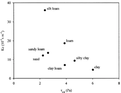
3-1 System elements (in circles) and processes (in rectangles) of the land-scape considered in this work. The forcings are represented with rounded corners boxes. . . . . 46 3-2 Parameter values of ra and Tc for different textures, assuming Pd = 1,

from Knapen et al. [2007] . . . . 62 3-3 Schematic representation of the bi-directional interaction between

ge-omorphological and hydrological processes, shown by thick dashed ar-rows, and the schematic representation of the bi-directional interac-tion between vegetainterac-tion dynamics and hydrological processes, shown by thick dotted arrows. . . . . 65 3-4 Impacts of vegetation on the bi-directional interaction between

geo-morphological and hydrological processes (see Figure 3-3), represented with thick solid arrows, and impacts of the land surface form and soil depth on the bi-directional interaction between vegetation dynam-ics and hydrological processes (see Figure 3-3), represented with thick dotted arrow s. . . . . 66 3-5 Soil moisture loss rates as a function of soil moisture for typical soil

and vegetation characteristics of semiarid ecosystems [Collins, 2006]. 69 3-6 Daily average of Th, Td, as a function of daily temperature. Hourly

temperature data used corresponds to the Kendall site, between 1997 and 2007. ... ... .... 80 4-1 The red square is the area within the WGEW considered in the

esti-mation of the NDVI time series presented in Figure 4-5 . . . . 87

4-2 Measurements at the Kendall meteorological station, 1997-2006 . . . 88 4-3 Moisture measurements at 5 cm, 1990-2007 . . . . 89 4-4 Runoff at subwatershed 112 of WGEW, 1999-2008 . . . . 89 4-5 NDVI from MODIS Terra, 2000-2006 . . . . 89

4-6 Minimum (pink) and maximum (red) temperatures during each day of 1999 at Kendall. A blue line represents the mean daily temperature, and a black line the representation of daily temperature used in CHILD. 90 4-7 Annual precipitation at Kendall and Lucky Hills, WGEW, 1997-2005 90 4-8 Location of the moisture measurements and soil sampling sites at

Kendall. The figure schematically represents a cross section of a small catchment in the Kendall site, with the north facing hillslope on the

right side of the figure and the south facing hillslope on the left. . . . 93 4-9 Vertical profile of soil at the Kendall site: a) vertical profile of soil

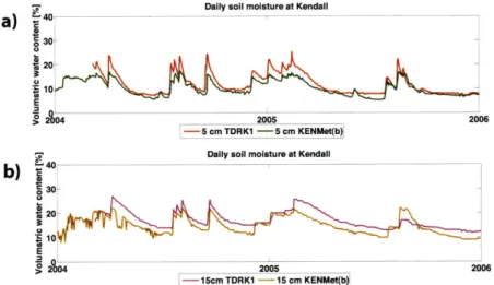
texture measured at two soil sampling pits, and location of soil moisture measurements; soil texture corresponding to different depths of the pits in b) the hillslope and c) the ridge is indicated with colored dots in a soil texture classification triangle. Dot colors correspond to colors of layers in a). . . . . 94 4-10 Moisture measurements at KENMet and TDRK1 between 2004 and

2005 at (a) 5 and (b) 15 cm depths. . . . . 95 4-11 Moisture measurements at KNTrench (a and b) and KSTrench (c) at

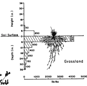
various depths (1991-1999). . . . . 96 4-12 Root distribution of grasses measured in the region of study, extracted

from Cox et al. [1986]. . . . . 97 4-13 Biomass estimated from NDVI at Kendall (2000-2006). The first

es-timation assumes that the maximum NDVI observed in the period of record corresponds to a full vegetation cover, which is assumed to be

0.2 kgDM/m 2. The second estimation assumes that an NDVI of 0.6

corresponds to a full vegetation cover. This figure also shows the to-tal precipitation of each year illustrating that biomass is not directly correlated to annual precipitation. . . . . 98 4-14 Above ground and below ground biomass estimated with the model

and that estimated from NDVI. . . . . 99 4-15 Comparison of simulated and measured moisture (measurements at 5

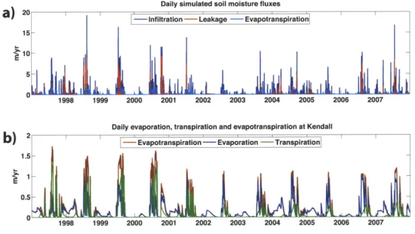
and 15 cm depths from a) TDRK1 (2004-2007) and b) KENMet (1997-2007)), c) evapotranspiration (measurements between 1997 and 2005), and d) runoff (measurements between 1999 and 2007). . . . . 100 4-16 Simulated soil moisture fluxes: a) shows infiltration, leakage and

evapo-transpiration; and b) the two components of evapotranspiration, namely evaporation and transpiration. . . . . 101 4-17 Comparison of simulated and measured a) moisture (at 5 and 15 cm

depths from KENMet) and b) evapotranspiration, at Kendall (2003). 102 4-18 Comparison of simulated and measured a) moisture (at 5 and 15 cm

4-19 11 years time averaged relative biomass as a function of drainage area, for the modeling results. Four different times of the year were sampled for this analysis: January 1, April 1, July 1 and October 1. . . . 105 4-20 11 years time averaged relative biomass as a function of aspect, for the

modeling results. Four different times of the year were sampled for this analysis: January 1, April 1, July 1 and October 1. . . . . 106 4-21 11 years time averaged relative biomass as a function of slope, for

ter-rain facing south, west, north and east, corresponding to the modeling output. Four different times of the year were sampled for this analysis: January 1, April 1, July 1 and October 1. . . . . 107 4-22 Map of drainage area of the watershed used in the simulation. The

values are of the logio of the drainage area, so that dark blue represents approximately 1000 000 m2 _{and green 1000 m}2_{. . . . . 108}

4-23 Map of aspect of the watershed used in the simulation. . . . . 109 4-24 Map of slopes of the watershed used in the simulation, the slope is in

degrees. ... ... 109 4-25 Moisture fluxes in and out of the soil in simulations of Kendall

con-ditions (1997-2007) under different soil textures: sand, clay and silty loam ... ... . . . .. ... .... . . . .. .. ... 117 4-26 a) Moisture and b) evapotranspiration in simulations of Kendall

con-ditions (1997-2007) under different soil textures: sand, clay and silty loam .. . . . .. . . .. . . ... .. . . .. .. 118 4-27 a) Above ground biomass and b) runoff in simulations of Kendall

con-ditions (1997-2007) under different soil textures: sand, clay and silty loam . . . . 118 5-1 Scheme of the landscape system represented with CHILD. In the figure

arrows indicate the direction of interaction among the various system components (elements and processes). Different colors indicate distinct feedback loops as labeled and described further in Table 5.1. Various arrows in one direction from one system component to another indicate that that connection forms part of more than one feedback loop, and not various connections. . . . . 120 5-2 Scheme of the landscape system represented by former landscape

evo-lution m odels. . . . . 121 5-3 Maps of the properties of Topo2: a) drainage area (the values are of the

log1O of the drainage area, so that dark blue represents approximately 10 000 m2 _{and yellow 25 m}2

), b) aspect, and c) slope in degrees. . . . 122

5-4 Scheme of the landscape system represented with CHILD in the static vegetation scenario. . . . . 124

5-5 Scheme of the landscape system represented with CHILD in the bare surface scenario. . . . . 124 5-6 Rainfall used to force CHILD in a 33 year simulation: a) historical

and b) Barlett-Lewis (BL) generated rainfall. The BL rainfall shown corresponds to individual storms. In the BL generated rainfall, within each storm, rainfall intensity varies (not shown). . . . . 125 5-7 Time series of above ground and root biomass for two simulations, one

using historical rainfall, and the other one using BL generated rain-fall (1997-2007). The above ground biomass shown corresponds to the basin averaged biomass for each time step. Root biomass shown

corre-sponds to the mean north facing terrain root biomass every 0.25 years. In these simulations mean north and south facing terrain biomass is sim ilar. . . . . 126 5-8 Annual accumulation of precipitation, infiltration, evaporation,

tran-spiration and leakage in the basin in meters: a) using daily observed rainfall and b) using the BL algorithm. The initial topography in this

simulation corresponds to the Kendall basin DEM with a 30 m resolution. 127 5-9 Above ground (AG) biomass in north and south facing terrain

through-out 33 three years of simulation in CHILD, corresponding to current cli-matic conditions at the Kendall site: a) using a constant WUE and b) using a WUE that changes with temperature. The initial topography in this simulation corresponds to the synthetic field Topo2 described below in the experimental set up. . . . . 128 5-10 Time averaged vegetation cover fraction in the synthetic field Topo2

(see the experimental set up section below) for the 33 year simulation in CHILD, corresponding to current climatic conditions at the Kendall site using a WUE that changes with temperature, at the beginning of a) spring, b) summer, c) fall and d) winter. . . . . 129 5-11 Precipitation and the ratio between annual evaporation and

transpi-ration (E:T) corresponding to a) the same simulation depicted in Fig-ure 5-8b, and b) the same simulation, but with a static or constant vegetation equal to the average AG vegetation cover of a). . . . . 130 5-12 Time series representing the root and leaf biomass in the a) dynamic

vegetation and b) revegetation scenarios of the simulations correspond-ing to Topol. The figure shows the north and south aspect averaged root and leaf biomass at 0.25 year intervals, and the basin averaged leaf biomass at every time step of the simulation. The root and leaf biomass are presented in separate graphs of different scales in the y

5-13 Time series representing the root and leaf biomass in the a) dynamic vegetation and b) revegetation scenarios of the simulations correspond-ing to Topo2. The figure shows the north and south aspect averaged root and leaf biomass at 0.25 year intervals, and the basin averaged leaf biomass at every time step of the simulation. The root and leaf biomass are presented in separate graphs of different scales in the y

axis because their. magnitudes differ by one order of magnitude. . . . 132 5-14 Regolith depth after 5 000 and 10 000 years for 5 different scenarios

corresponding to Topol.. . . . . . . . . 134 5-15 Total erosion and deposition (net changes in elevation) during 5 000

years for four different scenarios starting with Topol. Positive values (warm hues) indicate erosion, and negative values (cool hues) deposition. 135 5-16 Bedrock erosion in 5 000 years corresponding to four different scenarios

starting with Topol. . . . . 136 5-17 Regolith depth after 5 000 and 10 000 years of simulation for the 5

different scenarios considered in Table 5.2 starting with Topo2. . . . . 137 5-18 Changes in elevation in 5 000 years for the different scenarios starting

with Topo2. Positive values (warm hues) indicate erosion, and negative values (cool hues) deposition. . . . . 138 5-19 Bedrock erosion in 5 000 years for the different simulation cases starting

w ith Topo2. . . . . 139 5-20 Root biomass distribution corresponding to Topol dynamic vegetation

scenario at year 10 000, in kg/m 2. The color bar in a) shows the total

range of root biomass values, where as the color bar in b) shows a narrower range of values to make clearer the difference among north and south facing hillslopes. . . . . 140 5-21 Root biomass distribution corresponding to the Topol revegetation

scenario at year 10 000, in kg/rm2 . . . . . . . . . . . . . 141 5-22 Root biomass distribution corresponding to the Topo2 dynamic

vege-tation scenario at various times along the simulation, in kg/rm2. The

top panels are top views of the simulation, where as the bottom panels are views from the east into the simulation domain. The color scale of the bottom panels shows a reduced range in root biomass values to highlight differences in vegetation values within that range. . . . . 142 5-23 Root biomass distribution corresponding to the Topo2 revegetation

scenario at various times along the simulation, in kg/rm2_{. The top}

panels are top views of the simulation, where as the bottom panels are views from the east into the simulation domain. The color scale of the bottom panels shows a reduced range in root biomass values to highlight differences in vegetation values within that range. . . . . 143

5-24 Bedrock erosion distribution corresponding to the last 5 000 years of the Topol bare surface scenario, in meters. . . . . 144 5-25 Maps of erosion and sedimentation corresponding to the last 5 000

years of the Topol revegetation scenario, in meters. Positive values mean erosion, and negative values deposition. a) Absolute erosion and deposition , b) bedrock erosion only. . . . . 145 5-26 Slope area diagram for each scenario starting with Topol. The light

blue and dark blue dots represent the initial and final conditions of each mesh element of the model, respectively. Yellow and red circles linked with lines correspond to the mean slope for different drainage areas of the initial and final conditions, respectively... . . . ... 148 5-27 Slope area diagram for each scenario starting with the Topo2. The

light blue and dark blue dots represent the initial and final conditions of each mesh element of the model, respectively. Yellow and red circles linked with lines correspond to the mean slope for different drainage

areas of the initial and final conditions, respectively. . . . . 149 5-28 Differences in elevation after 10 000 years of simulation between the

dynamic vegetation and static vegetation scenarios that start with Topol. 150 5-29 Relative below ground biomass as a function of aspect at different times

during the dynamic vegetation scenario for Topol. . . . . 152 5-30 Relative below ground biomass as a function of slope at different times

during the dynamic vegetation scenario for Topol. . . . . 153 5-31 Relative below ground biomass as a function of drainage area at

dif-ferent times during the dynamic vegetation scenario for Topol. . . . . 154 5-32 Slope as a function of aspect for all scenarios (dynamic vegetation,

static vegetation, bare surface, degradation, revegetation) correspond-ing to a) Topol and b) Topo2. . . . . 155

LIST OF TABLES

3.1 Summary of the Barlett-Lewis parameters... . . . . . . . . 50

3.2 Range of values of Iid and r, for soils from different studies . . . . 63

3.3 Values of kd when Pd is different from 1 for the Lucky Hills site in W alnut Gulch, AZ . . . . 63

3.4 Differences between laboratory and field conditions in Kd . . . . 64

3.5 Measured values of water use efficiency (WUE) for grasses and grass communities [Scholes and Walker, 1993] . . . . 73

3.6 Parameters for the vegetation model from various sources . . . . 78

4.1 Meteorological, soil moisture and NDVI data sets . . . . 86

4.2 Summary of soil properties from two soil pits at Kendall . . . . 92

4.3 Summary of soil properties for sand, clay and silty loam, used in the sim ulations . . . . 116

5.1 Feedback loops described in Figure 5-1 . . . . 120

5.2 Set of experimental runs carried out with CHILD . . . . 123

A.1 Model parameters, solar forcing . . . . 165

A.2 Model parameters, geomorphic processes . . . . 166

A.3 Model parameters, hydrologic processes . . . . 166

A.4 Model parameters, vegetation dynamics, Chapter 4 . . . . 167

A.5 Model parameters, vegetation dynamics, Chapter 5 . . . . 167

CHAPTER 1

INTRODUCTION

AND BACKGROUND

1.1

Introduction

Vegetation modifies the hydrologic and geomorphic properties of the land surface and as a result geomorphic processes modify the surface at different rates under differ-ent vegetation covers. Plant developmdiffer-ent, in turn, largely depends on topographic organization. This dependency is shown in the fact that different plant communities develop across different topographic settings. Thus, the evolution of land features such as mountains, rivers, and valleys is intimately related to the development of plants.

Despite the evident interdependence between vegetation and topography, little is known about how vegetation and topography co-evolve to produce the landscapes we observe today, if indeed they do, and to what extent the interplay between topography and vegetation affects the evolution of a landscape. The development and use of a physically based model that represents the topography-vegetation interaction during their simultaneous evolution can greatly improve our understanding of this matter. Such a model would allow a more realistic representation of both, topographic evo-lution and vegetation community development.

This thesis investigates the interdependence between the evolution of topography and vegetation in water-limited ecosystems by means of physically based numerical simulation. The numerical model considers the following factors: vegetation controls on water flux on a basin and on erosion-deposition processes, topography controls on moisture fluxes, and soil moisture controls on vegetation dynamics. The above factors are analyzed under a dynamic topography framework.

The spatial scale addressed in this study is that of small drainage basins, between 0.01 to 4 km2. The temporal scales addressed are two. The evolution of topography

is analyzed in thousands of years; the evolution of vegetation is analyzed in more detail at yearly time scales.

The Channel-Hilllsope Integrated Landscape Development (CHILD) model was modified to enable the representation of the interaction of vegetation and topography. The model additions of moisture and vegetation dynamics are tested by comparing its outputs to observations. Digital maps of topography and vegetation are also analyzed to search for correlations between the spatial distribution of vegetation and topographic attributes of the land surface. These correlations serve as a basis of comparison for the modeling.

The objective of this work is to evaluate the effects of the interplay between vegetation and topography in the evolution of a small drainage basin. Quantitative answers to the following questions are investigated:

1. Do current landforms result from the topography-vegetation interaction, or would landforms have evolved to their present condition without this interaction?

2. Have current vegetation communities in a landscape adapted to the present topographic conditions and reached a steady state (which corresponds to the contem-porary topography and climate)? Is this steady state dependent upon or independent of the history of the topography-vegetation interaction?

3. Assuming a topography-vegetation interaction, how sensitive are the processes acting on a landscape to external disturbances in climate and land cover? How sensitive is the steady state of a landscape to these external disturbances?

1.2

Background

Ridges, hillslopes and streams are topographic elements that together with plants and soil properties constantly interact through hydrologic processes within a system enclosed in a drainage basin. Strong interdependencies exist between these topo-graphic elements and basin hydrology, between plants and basin hydrology, and as a consequence of these first two, there is an interdependence between basin topog-raphy and plants. The above interdependencies have been extensively studied and documented, and below a brief review is presented to emphasize the relevance of each of the elements considered in the modeling work and to justify the modeling considerations.

1.2.1

Interdependence of topographic features and hydrology

Changes in landforms significantly depend on the amount and direction of water flow across a basin (basin hydrology). Conversely, flow on a basin is predominately controlled by topography [Huang et al., 2002; Rodriguez-Iturbe and Valdes, 1979].

Rates of topographic denudation are commonly considered proportional to the shear stress that flowing water (or wind) exerts on a surface. Thus, geomorphic processes are most intense where the largest amounts of water discharge concentrate, and where flow velocities are highest (i.e., where the slope is steepest and smooth).

It is along those areas where the most rapid changes in landforms occur.

Topography directs the surface water fluxes and affects the concentrations, velocity and distribution of flow in time and space across a basin. Concave hillslopes cause convergence of flow while convex hillslopes induce divergence. Water flow velocity increases with hillslope and channel steepness. The distribution of a basins outflow in time depends on the shape of the basin and on the distribution of its channel network. For example, in elongated basins flow will be more uniformly distributed than on rounded basins [Surkan, 1969].

1.2.2

Interdependence of vegetation and hydrology

The establishment of vegetation on the landscape is determined in more than one way by the fluxes of water [Rodriguez-Iturbe and Porporato, 2005]. The availability of water in the land surface is a limiting factor in plant development, as either excess or scarcity can prevent their existence. Water availability, thus, is responsible for the variety of plant communities found on terrestrial landscapes (e.g., Shmida and

Burgess [1988]). Fluxes of water also affect plant development. Large amounts of flux

through the soil can decrease nutrient availability through leaching, thus limiting plant growth. Large amounts of flow on the surface can damage plants. As a consequence, only the few plants that survive floods or that rapidly regenerate can develop in zones where floods frequently damage vegetation [Sigafoos, 1961; Scatena and Lugo, 1995]. Evidence of this interdependence has been observed where man has altered the natural state of a basin. For example, changes in the hydrologic response of a basin due to dam control result in changes in vegetation over the course of years [Johnson

et al., 1976].

The fluxes of water in a basin are affected in various ways by vegetation. On a lo-cal slo-cale vegetation affects the roughness of the surface, thus, horizontal water fluxes across the land are slower on vegetated surfaces [Abrahams et al., 1995]. Vegetation also affects the vertical fluxes of water on the land by canopy interception, enhance-ment of the surface's infiltration capacity and water store capacity, and transpiration (e.g., Selby [1970]; Wistendahl [1958]; Mosley [1982]; Aldrige and Jackson [1968]). Because of the transformations described above, changes in vegetation immediately after fires, for example, result in new hydrologic basin responses

[

Wistendahl, 1958; Gurnell et al., 1990; Francis and Thornes, 1990; Moody and Martin, 2001; Benavides-Solorio and MacDonald, 2001].

1.2.3

Interdependence of topographic features and vegetation

Topography can control the development and spatial distribution of vegetation, while vegetation influences erosion and deposition of soil and hence may exert a feedback on topography. As is shown below, the signals between topographic development and plant development are transmitted through the hydrologic processes of the basin.

Topographic controls on vegetation development

Vegetation development is largely controlled by the amount and distribution in time of water available to plants. Water availability is often responsible for differences among plant community (e.g., grasslands, savannas, forests) [Rodri'guez-Iturbe and

Porporato, 2005]. Therefore, vegetation development is often considered mainly a

function of water stored in the soil. The amount of water stored in the soil is mea-sured as soil moisture. Soil moisture is the percentage, in volume, of soil pores filled with water. The amount of water stored in the soil depends on climate, soil character-istics, vegetation, and topography. In relation to climate, Shmida and Burgess [1988] show a general link between precipitation and ecosystem type, biomass and biodi-versity. Several studies have shown an increase in plant recruitment with holding capacity [Lauenroth et al., 1994]. Soil depth and texture have been recognized as key factors in soil water holding capacity and vegetation development [Porporato et al., 2001; Lazo et al., 2001a]. Vegetation affects the inputs and outputs of water from soil in several ways, for example, it significantly modulates infiltration rates [Selby, 1970], intercepts rainfall [Lull, 1964], and regulates rates of evapotranspiration (e.g., Molchanov [1971]). Topography affects soil moisture distribution on the hillslope scale [Ridolfi et al., 2003] and on the basin scale [Hack and Goodlett, 1960]. Concave and topographically convergent regions are generally moister than convex and diver-gent regions. Aspect, the orientation of a hillslope with respect to the geographic north, is a characteristic of topography that often has been related to vegetation and soil development [Hack and Goodlett, 1960; Kirkby et al., 1990; Hidalgo et al., 1990]. Vegetation development is also controlled by erosion. Frequency of damaging floods in different sections of the landscape affect the distribution of vegetation species and age distribution of plants across a basin. Scatena and Lugo [1995] and Basnet [1992] describe species and age distribution of trees in a tropical basin in Puerto Rico, where ridges have older trees than valleys. Valleys are frequently disturbed by floods and have trees and species that reproduce rapidly. Hack and Goodlett [1960] and

Teversham and Slaymaker [1976] describe patterns of plant community distribution

in a basin that are correlated to the frequency of flood disturbances.

Vegetation controls on geomorphic processes

Experiments and measurements in flumes and plots have shown the impact of vege-tation cover on runoff and sediment yield, where sediment yield is not only a function of the runoff produced shear stress, but also a function of the erodibility of the soil and of the deposition of soil where vegetation acts as a barrier against flow (e.g.,

Abrahams et al. [1995]; Vacca et al. [2000]; Rey [2003]; Trimble [1990]; Sorriso-Valvo et al. [1995]). Vegetation reduces soil erodibility [Reid, 1989; Prosser and Dietrich, 1995; Prosser and Slade, 1994] and is responsible for altering soil chemistry leading to enhanced resistance to erosion [Angers and Caron, 1998; Viles, 1990]. Plants also provide soil with cohesive strength by means of their roots [Greenway, 1990;

rain splash protection and rainfall interception [Abrahams et al., 1995; Aldrige and

Jackson, 1968]. Finally, plants offer resistance and protection against the flow of water or air, thus decreasing the shear stress exerted on the soil [Prosser and Slade,

1994].

In addition to the effects of vegetation on the erosion of the landscape by wa-ter flow, vegetation (together with other living organisms) enhances weathering and thus soil production. However, if the weathered material is not retained, it leads to denudation (e.g., Yair [1995]).

Because of the significant effect of vegetation on water flow, and as a consequence on geomorphic processes and landform evolution, a detailed representation of water flow is critical to capture the effects of vegetation on geomorphic processes. Impor-tant progress has recently been made in estimation of flow on small basins taking into account the heterogeneity of rainfall and surface properties, including soil moisture conditions [Ivanov et al., 2004]. Field and numerical evidence show the importance of temporal and spatial variability in precipitation and flow across a basin on geomor-phic processes [Molndr and Rami'rez, 2001; Sdlyom and Tucker, 2004]. These results reinforce the importance of resolving flow variation in time and space when modeling landscape evolution.

The interdependencies between topographic features and hydrology, plants and hydrology, and topographic features and plants, have profound implications on the evolution of a landscape. This work expands the understanding of the integration of all three in landscapes.

1.2.4 Modeling of landscape evolution

The interactions between landforms and vegetation through hydrologic and geomor-phic processes have been described qualitatively, based mostly on field observations from small scales (e.g., the size of a plant) to larger scales (e.g., the size of a basin). These interactions are numerous, they occur in a three-dimensional space and in a wide range of temporal scales. In order to elucidate the feedbacks that are most important in landscape evolution, we need to isolate variables, change initial and boundary conditions, and measure responses to these changes in a well-controlled environment. Numerical modeling has been one of the preferred tools to do so and will be the main tool of study in the proposed work. Before describing the modeling approach for this work, a brief summary of the efforts of numerical modeling in the field of landscape evolution is provided.

Development of numerical models to simulate soil erosion and landscape evolution based on water fluxes across the surface, tectonic uplift, sediment deposition, mass wasting, and even Martian geomorphic processes is highly advanced (e.g., Howard [1988, 1994]; Tucker and Bras [1998]; Tucker et al. [2001]; Willgoose et al. [1991]). A review of contemporary basin evolution models is given in Coulthard [2001]. Numeri-cal models that simulate vegetation growth by considering nutrients, climate, and in-ternal plant dynamics on various scales have provided surprising new understanding of

plant community development and response to natural and human disturbances (e.g.,

Moorcroft et al. [2001]). Others have used numerical modeling to study specifically

the interactions between vegetation growth and soil moisture (e.g., Rodriguez-Iturbe

et al. [2001]). The modeling of hydrologic processes taking into account the effects

of vegetation is constantly improving. One such model, tRIBS, considers spatial het-erogeneity and temporal variability in hydrometeorological forcing (e.g., rainfall) and land surface characteristics, which include soil moisture and vegetation cover [Ivanov

et al., 2004]. Recent developments of this hydrologic model incorporate the dynamic

development of plants. Results show that topography affects plant development by regulating soil water and energy budgets. In the model the surface and subsurface flow of water are by and large controlled by topography, and energy fluxes and wa-ter evapotranspiration are largely controlled by solar radiation, dependent on aspect

and slope of the terrain. In model simulations, for example, plants grow at different rates on opposing sides of a ridge due to differences in exposure to solar radiation, and biomass production is distinctively higher in plants growing in channels than in plants growing in hillslopes. In tRIBS, however, topography does not change in time

[Ivanov et al., 2008a].

The study of the interaction between landforms and vegetation through geomor-phic and hydrologic processes has also evolved. Some models that represent basin scale landform evolution have incorporated the effects of vegetation to a certain ex-tent. Some examples are SIBERIA and GOLEM [Willgoose et al., 1994; Tucker and Slingerland, 1996], Howard's [Howard, 1994] detachment limited model, and CHILD [Tucker et al., 2001]. The last has explored the role of vegetation on landscape

evo-lution in a simplified way, considering only the effects of vegetation on the erodibility properties of the surface. Until recently, vegetation dynamics in CHILD had been only a function of space available for growth and erosion (which kills the plants) [Collins

et al., 2004]. Coulthard et al. [2002] developed a model that represents landscape

evolution at fine spatial and temporal scales (3 m grid cells and time steps within rainfall events) in which vegetation affects the flow and where vegetation growth is a function of erosion and time of recovery only. Kirkby et al. [2002] have developed a model (MEDRUSH) designed to estimate runoff and sediment yield from Mediter-ranean landscapes on scales of 100 years. In this model, a sophisticated vegetation component that modifies the soil properties and the thus the hydrologic and geo-morphic processes has been included. This model, however, does not consider any topographic change. Istanbulluoglu and Bras [2006] devised a point model that esti-mates the erodibility of soil as a function of the state of vegetation on the surface. In their model vegetation growth and death is a function of plant stress due to water availability. Water availability is estimated through a soil water balance where the infiltration process, canopy interception and evapotranspiration are all functions of the state of vegetation. The principles employed by Istanbulluoglu and Bras [2006] to simulate the development of vegetation and vertical fluxes across the land surface are used in the modeling work proposed here. Istanbulluoglu and Bras [2005] analyzed the response of a landscape under a uniform vegetation cover under different tectonic uplift rates and rainfall. From such analysis it was concluded that the dominant

ge-omorphic process depends on the combination of the three elements: tectonic uplift, vegetation cover, and rainfall. Istanbulluoglu and Bras [2005] also simulated vegeta-tion development in a landscape under a climate characteristic of the Oregon Range Coast using a simple vegetation development model independent of soil moisture in CHILD. They compared the landscape evolving with a vegetation cover to an unveg-etated landscape. The vegunveg-etated landscape had a high and steep relief with a small drainage density that contrasted with the unvegetated landscape, which displayed low relief, gentle slopes and higher drainage density.

The modeling efforts discussed above have not captured the implications of the vegetation-topographic features interdependence described in the preceding section. This work takes advantage of all the previous modeling efforts in this area (CHILD is modified), to capture such interdependence.

1.3

Thesis outline

The thesis is comprised of 6 chapters, including this Introduction. Chapter 2 presents an analysis of the links between vegetation, radiation and topography for two sites in semi-arid grasslands, the environment that is the focus of this work. For the analysis a series of measures to quantify the distribution of vegetation as a function of topographic attributes were developed. These measures are later used to compare modeling outputs with observations in Chapters 4 and 5.

Chapter 3 presents CHILD and its new capabilities. These new capabilities in-clude a new Barlett-Lewis rainfall generation algorithm that captures intra-storm variability, a critical component for the generation of runoff in semiarid regions. The latest version of CHILD also represents the seasonality of rainfall and of solar forcing. A characteristic of the new model is that its vegetation parameters are grounded on physical measurements that can be found literature. The fine temporal scale rep-resentation of climate and vegetation dynamics (including seasonality) allows for a direct comparison of the modeling to field or remote sensing observations of vegetation dynamics.

Moisture dynamics and their link to vegetation dynamics had been previously in-corporated into the model [Collins and Bras, 2008]. In that work transpiration was proportional to vegetation fractional cover, and vegetation dynamics followed a logis-tic growth equation whose colonization rate was proportional to transpiration, and death rate was proportional to a static water stress. In this work, the links between moisture and vegetation dynamics are similar, yet the logistic equation is not used to represent the vegetation dynamics. This work uses the water use efficiency (WUE) concept, which has been frequently employed in the agricultural community and in ecological studies. In this work, furthermore, moisture and vegetation dynamics re-flect the differences in solar incidence angle due to the form of the terrain.

Chapter 4 discusses the controls of climate, topography and soil properties on vegetation dynamics, and compares the vegetation and soil moisture representations

of CHILD with measurements. The goal of the chapter is to validate the represen-tation of the vegerepresen-tation dynamics in CHILD and to acknowledge its capabilities and limitations. In Chapter 4 the duration of the simulations is a few years, and the geomorphic processes are turned off.

In Chapter 5 the evolution of the landscape over 10 000 years is simulated. Five different scenarios, and two different initial topographic settings are presented. In these simulations all the processes discussed in Chapter 3 are active on the landscape, including the geomorphic processes. The goal of this chapter is to investigate the role of vegetation dynamics on the evolution of land form, erosion and sedimentation in a basin.

Finally, Chapter 6 presents a summary and the main conclusions drawn from this work.

FEEDBACK

BETWEEN

CHAPTER 2

_VEGETATION

DISTRIBUTION

AND LAND

SURFACE FORM

ABSTRACT

The magnitude of the bidirectional interaction between landforms and vegetation is poorly understood. This work quantifies that feedback by elucidating correlations between vegetation and topographic attributes (aspect, slope, and drainage area) in two semiarid grasslands in the southwestern U.S. (one in Arizona and the other in New Mexico). Digital elevation models (DEMs), biomass maps, and Normalized Difference Vegetation Index (NDVI) maps, with data spanning several years, are used in the investigation.

Results indicate that vegetation is inversely proportional to topography-modulated radiation; vegetation is directly proportional to drainage area; and the protection pro-vided by vegetation cover results in steeper terrain.

At the Arizona site the effects of water accumulation along the drainage network conceal some of the topography-modulated radiation effects.

Finally, it is observed that the effects of topography on vegetation are relatively larger in the dry season preceding the monsoon, or early in the monsoon growing season.

2.1

Introduction

The heterogeneous distribution of vegetation in space affects the degree to which geomorphic processes act on the land surface. Given that geomorphic processes shape the land surface and distribute sediment, the above suggests that vegetation may affect landscape morphology. At a local scale, for example, grasses protect the surface against fluvial erosion [Prosser et al., 1995] and rain splash [Abrahams et al., 1995]. Furthermore, grasses increase surface roughness, reduce runoff rates [Abrahams et al., 1995; Prosser et al., 1995], allow for higher infiltration [Selby, 1993], and as a result,

diminish water erosive power. Grasses also trap sediment transported by water or wind [Abrahams et al., 1995; Lancaster and Bass, 1998]. At basin scales, vegetation removal is known to result in large changes in water fluxes and sediment [Bormann

and Liekens, 1979; Bosch and Hewlett, 1982; Selby, 1993].

Patterns of vegetation in the landscape are mainly a function of light, tempera-ture, and available soil moisture [Dick-Peddie, 1993; Bonan, 2002; Eagleson, 2002;

Larcher, 2003]. In this work it is argued that these factors are defined by climate

at a regional scale, and by landform and soil properties at a local scale. Therefore, at the local scale, vegetation and topography are likely to have a bidirectional in-teraction through biological and physical processes. Various documented examples of topographic relationships with vegetation distribution exist [Hack and Goodlett,

1960; Hidalgo et al., 1990; Basnet, 1992; Scatena and Lugo, 1995; McMahon, 1998],

as well as studies of the effects of vegetation on geomorphic and hydrologic processes

[Prosser and Slade, 1994; Abrahams et al., 1995; Prosser et al., 1995; Prosser and Dietrich, 1995; Collins et al., 2004; Istanbulluoglu and Bras, 2005; Gutierrez-Jurado

et al., 2007; Istanbulluoglu et al., 2008]. However, the magnitude of the bidirectional

interaction is not well understood.

In humid environments, light and nutrient availability are important limiting fac-tors for plant development, and in cold environments, temperature is a limiting factor. This work focuses on grasslands in a temperate semiarid region, where water availabil-ity is the main limiting factor for plant growth. Previous observations have noted that distinct vegetation establishes on north and south facing hillslopes in mid-latitudes and semiarid regions [Kennedy, 1976; Hidalgo et al., 1990; Gutiirrez-Jurado et al., 2006]. This is attributed to the effect of differences in radiation on north and south facing hillslopes, leading to differences in soil moisture and temperatures. Recently,

Ivanov et al. [2008a,b] reproduced distinct vegetation biomass distributions of grasses,

in a complex terrain mimicking semiarid central New Mexico. Their numerical model accounted for the impact of topography on vegetation establishment and growth, taking into account the effects of topography on radiation and soil moisture distri-bution. Results indicated that vegetation growth is limited on south facing hillslopes because of excessive radiation, stressing the plant by depleting soil moisture, and that north-facing hillslope conditions result in more abundant vegetation growth. Results also indicated that vegetation patterns follow the drainage network when a significant amount of rainfall runs off from hillslopes into the drainage network.

Recently, two studies of a semiarid site in central New Mexico attributed differ-ences in the geomorphic response and morphology of opposing north and south facing hillslopes to vegetation cover differences [Gutiirrez-Jurado et al., 2007; Istanbulluoglu

et al., 2008]. This work extends the previous investigations by analyzing the

rela-tionships between vegetation distribution and topographic attributes (aspect, slope and drainage area) in two grass-dominated semiarid sites, one called Kendall, within the Walnut Gulch Experimental Watershed (WGEW) in Arizona, where mean an-nual precipitation is 350 mm per year, and the other in the northwestern section of the Sevilleta National Wildlife Refuge (SNWR) in New Mexico, where mean annual

precipitation is substantially smaller, 250 mm per year. At both of these sites more than 50 % of the precipitation falls during the summer monsoon, when most of the vegetation growth takes place. Conditions previous to the monsoon are generally dry. In this study, grass species are treated as a single functional type. As a result, it identifies changes of the grass community as a single entity, not the species-specific responses of its component parts.

2.2

Field sites and data

2.2.1

Kendall site, southeastern Arizona

Kendall is a site dominated by grasses within the USDA-ARS Walnut Gulch Experi-mental Watershed (WGEW) (31'43'N, 110'41'W). The climate of this semiarid region is characterized by a mean annual precipitation of 350 mm, a mean annual temper-ature of 17.7 'C, an annual pan evaporation of 2590 mm, with a strong seasonality affecting the temporal distribution of these variables. The precipitation regime is dominated by the North American Monsoon, which occurs during the months of July through September, during which about two-thirds of the annual precipitation falls. The mean monthly temperature ranges between 8 'C in January and 27 'C in July

[Goodrich et al., 2008; Keefer et al., 2008].

Kendall is within an alluvial fan that forms part of the San Pedro River watershed, with elevations ranging between 1500 m and 1600 m AMSL. It is dominated by C4 perennial grasses, including black, blue, hairy and sideoats gramas (B. eripoda, B.

gracilis, B., hirsuta and B. curtipendula) [Nouvellon et al., 2001].

2.2.2

SNWR site, central New Mexico

The second site used in this study is the grass-dominated terrain within the rect-angular region of approximately 14 by 18 km in the northwest area of the Sevilleta National Wildlife Refuge (SNWR). The SNWR (34'24'N, 106'59'W) has a climate similar to that of Kendall, with more than 50 % of the annual precipitation falling during the North American Monsoon, and mean monthly temperatures ranging be-tween 2.5'C in January and 250C in July. However, significantly less precipitation falls in the SNWR; its mean annual precipitation is 250 mm [Milne et al., 2003].

The area selected for the study, with elevations ranging between 1450 and 2500 m AMSL, is formed by alluvial deposits, eolian sand deposits, terrace deposits, and Precambrian granite and metamorphic rocks. Most of the grass-dominated rugged terrain within this rectangle is underlain by the Sierra Ladrones, and its elevation is below 1700 m AMSL. The Sierra Ladrones is an outcrop of the Sierra Ladrones Formation east of the Loma Pelada Fault [McMahon, 1998].

woodlands and forests at the higher elevations [Dick-Peddie, 1993; Milne et al., 2003;

Muldavin et al., 1998]. The area used in this study is nevertheless dominated by

sev-eral grass species, including black (Bouteloua eripoda) and blue gramma (Bouteloua

gracilis) (Figure 2-1).

Non-grass cover Grass cover water

Figure 2-1: Map of the New Mexico site showing the DEM extracted drainage network with red lines, and the distribution of grassland, non-grassland covered terrain, and 'water' (the ephemeral Rio Salado).

2.2.3

Data

Data used in this analysis consist of Digital Elevation Models (DEMs) and maps of the spatial distribution of grasses. For the Arizona site (Kendall), a 1 m resolution DEM was used. This DEM was provided by personnel at the Tombstone Agricultural Research Service (ARS) office. For the New Mexico site, a 10 m DEM (EarthWatch Star-3i IFSAR product) of the region was used. This DEM is publicly available at http://sev.lternet.edu. Digital maps of slope, aspect and drainage area were obtained from the DEMs using Arcview.

Five digital maps of Normalized Difference Vegetation Index (NDVI) [Tucker, 1979], representative of the grass photosynthetic activity at the Kendall site, were used. These NDVI maps correspond to different dates spanning between August 24, 1990 through September 10, 1999, and have a spatial resolution of 30 m. These maps were obtained from NASA's Landsat Thematic Mapper (TM) images [Moran et al., 2008]. The images were geocorrected to subpixel accuracy, and the refined empirical line (REL) method [Moran et al., 2001] was used to convert dn to reflectance for the red and NIR spectral bands, as in Holifield et al. [2003].

Twenty-two grass biomass maps of the SNWR were used. These maps, publicly available at the SNWR website (http://sev.lternet.edu), correspond to various dates