HAL Id: hal-03049674
https://hal.archives-ouvertes.fr/hal-03049674
Submitted on 9 Dec 2020HAL is a multi-disciplinary open access archive for the deposit and dissemination of sci-entific research documents, whether they are pub-lished or not. The documents may come from teaching and research institutions in France or abroad, or from public or private research centers.
L’archive ouverte pluridisciplinaire HAL, est destinée au dépôt et à la diffusion de documents scientifiques de niveau recherche, publiés ou non, émanant des établissements d’enseignement et de recherche français ou étrangers, des laboratoires publics ou privés.
Acid/base front propagation in saturated porous media:
2D laboratory experiments and modeling
Stéphanie Lawniczak, Francois Lehmann, Philippe Ackerer
To cite this version:
Stéphanie Lawniczak, Francois Lehmann, Philippe Ackerer. Acid/base front propagation in saturated porous media: 2D laboratory experiments and modeling. Journal of Contaminant Hydrology, Elsevier, 2012, 138-139, pp.15-21. �10.1016/j.jconhyd.2012.06.005�. �hal-03049674�
Acid/base front propagation in saturated porous media: 2D laboratory
1experiments and modeling.
23
Stéphanie Loyaux-Lawniczak, François Lehmann and Philippe Ackerer*
4 5
Laboratoire d’Hydrologie et de Géochimie de Strasbourg, 6
Université de Strasbourg/EOST – CNRS, 7
1 rue de Blessig, 67000 Strasbourg, 8
France. 9
10
* Corresponding author. E-mail address: [email protected] 11 12 13 Abstract 14 15
We perform laboratory scale reactive transport experiments involving acid-basic reactions 16
between nitric acid and sodium hydroxide. A two-dimensional experimental set-up is 17
designed to provide continuous on-line measurements of physico-chemical parameters such as 18
pH, redox potential (Eh) and electrical conductivity (EC) inside the system under saturated 19
flow through conditions. The electrodes provide reliable values of pH and EC, while sharp 20
fronts associated with redox potential dynamics could not be captured. Care should be taken 21
to properly incorporate within a numerical model the mixing processes occurring inside the 22
electrodes. The available observations are modeled through a numerical code based on the 23
advection-dispersion equation. In this framework, EC is considered as a variable behaving as 24
a conservative tracer and pH and Eh requires solving the advection dispersion equation only 25
once. The agreement between the computed and measured pH and EC is good even without 1
recurring to parameters calibration on the basis of the experiments. Out findings suggest that 2
the classical advection-dispersion equation can be used to interpret these kinds of experiments 3
if mixing inside the electrodes is adequately considered. 4
5
1. Introduction
1 2
Modeling reactive transport of dissolved species in porous media is considered essential in 3
Earth sciences and has been the subject of several investigations (e.g., Steefel et al., 2005 and 4
references therein). Prediction of migrating reactive chemicals (including, e.g., heavy metals, 5
organic species from industrial solvents, products from mining, agrochemicals, 6
petrochemicals) is also of paramount concern for the protection, management and remediation 7
of groundwater resources. 8
Several numerical techniques and codes have been developed to simulate reactive transport 9
processes in natural groundwater systems (Kinzelbach et al., 1991; Yeh, & Tripathi, 1991; 10
Walter et al., 1994; Saaltink et al., 2001; Van der Lee et al., 2003; Fahs et al., 2009 among 11
others). The mechanisms involved in reactive transport processes are often strongly non-linear 12
and occur on a multiplicity of time scales, thus rendering the solution of a mathematical 13
model very challenging. Verifying and assessing the robustness of numerical models can be 14
performed by benchmarking. However, recent results have shown that different numerical 15
schemes and codes can produce different results for the same benchmark problem even under 16
apparently simple one-dimensional scenarios (Carrayrou et al., 2010). 17
Assessment of the reliability of conceptual schemes and associated computational models can 18
also be performed through controlled experimental investigations at the laboratory scale. 19
There is a vast literature devoted to analyzing experiments performed within seemingly one-20
dimensional porous systems, obtained by packing granular material within columns of 21
different length scales (Burris et al., 1996; André et al., 1998; Gandhi et al., 2002; Gramling 22
et al., 2002; Su & Puls, 2004; Grolimund & Borkovec, 2006, among many others). Two-23
dimensional set-ups have been used only recently to observe key features of reactive transport 24
experiments, with special emphasis on transverse mixing processes in the presence of fluids 25
with different water compositions. Experiments have documented the precipitation pattern of 1
a calcium carbonate solid phase (Katz et al., 2010), concentration distributions in 2
heterogeneous density-driven flow systems (Konz et al., 2009a), biodegradation of toluene 3
(Bauer et al., 2008), and transverse mixing in heterogeneous porous media (Rolle et al., 4
2009). 5
Detailed reactive transport experiments are also required to improve our understanding of the 6
main features of spreading and mixing processes affecting solutes migration at different 7
scales. Characterization of conservative or reactive transport via Fickian or non-Fickian 8
models is still an open debate. For example, the reactive transport experiments of Gramling et 9
al. (2002) involving an irreversible bimolecular reaction could be interpreted by particle 10
tracking methods relying on non-Fickian solute behavior (Edery et al., 2009, 2010) or by 11
solving a continuum model based on the standard advection-dispersion-reaction equation 12
(ADRE) with a time-dependent macro-scale kinetic term describing mixing of solutes at the 13
small scales (Sanchez-Vila et al., 2010). A review of the role of small scale concentration 14
fluctuations in the interpretation of laboratory scale experiments is presented by Edery et al. 15
(2012). 16
Solutes concentrations and/or physico-chemical variables (e.g., pH, electrical conductivity) 17
are typically measured at the outlet of the flow cell (Chiogna et al., 2010), by sampling small 18
volumes of water inside the porous material (Katz et al., 2010), or indirectly by image 19
analysis of colorimetric reactions (Zinn et al., 2004; Jones & Smith, 2005; Konz et al., 20
2009b). Monitoring at the outlet usually provides only information which is representative of 21
some cross-sectionally averaged behavior. Direct sampling within the flow cell cannot be 22
repeated too frequently without significantly perturbing the flow and transport conditions, and 23
indirect measurements based on imaging techniques are limited to some specific solutes and 24
reactions. 25
To our knowledge, protocols for extensive direct measurements of concentrations and/or 1
physico-chemical parameters inside a porous medium have not been implemented, with the 2
exception of applications related to measurements of dissolved oxygen (Chiogna et al., 2010). 3
Although such measurements are not easy to accomplish, they are required to firmly ground 4
modeling interpretations on space distributed observation dynamics. 5
A key aim of this study is to present a set of laboratory-scale experimental tools and a 6
methodological approach conducive to an improved characterization of flow and transport 7
patterns within natural systems through continuous on-line measurements of parameters such 8
as pH, redox potential (Eh) and electrical conductivity (EC). These local measurements are 9
performed inside the porous medium under imposed flow-through conditions. A user-defined 10
time resolution allows (a) obtaining detailed records of point breakthrough curve, and (b) 11
exploring a wide range of experimental time scales. 12
The two-dimensional (2D) experimental set-up, the mathematical model and the associated 13
numerical solution scheme employed to interpret the experimental evidences are presented in 14
Section 2. The main features of the three experiments performed are described in Section 3. 15
Section 4 is devoted to illustrating the modeling results. 16
17
2. Materials, Methods and Modeling
18 19
2.1. Experimental set-up 20
21
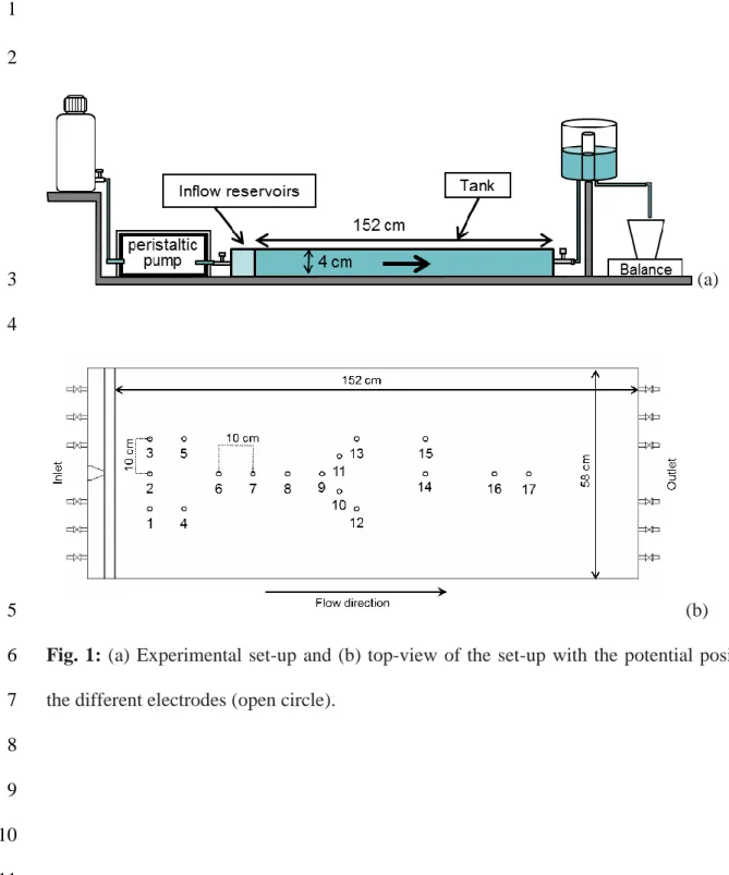
An Altuglas® flow cell (external dimensions: length 167-cm, width 68-cm, and thickness 4-22
cm) was divided into two compartments consisting of a 5-cm long inflow reservoir and a 152-23
cm long compartment containing the porous medium (hereafter termed the ‘tank’) as depicted 24
in Fig. 1. The two compartments were separated by an Altuglas® plate with porosity 0.37 25
resulting from regularly spaced 8-mm diameter holes. A 50-µm nylon filter was used to 1
prevent the porous medium from invading the inflow reservoir. This inflow reservoir was 2
divided into two identical and independent sub-reservoirs to allow the simultaneous injection 3
of two different solutions in parallel. The injection into each sub-reservoir was performed by 4
3 tubes to optimize mixing inside the sub-reservoir and a Masterflex® L/S 2-channel 5
peristaltic pump to prevent flow rate differences between the sub-reservoirs. Six tubes 6
connect the outlet side of the tank to an outflow reservoir. The flow rate was regularly 7
controlled by on-line weighing of the solutions collected at the outflow. 8
9
The tank was filled up with glass beads (SiLibeads®, Sigmund Lindner, GmbH), which had a 10
narrow size distribution and a diameter ranging from 0.5 to 0.75 mm. Glass beads were used 11
rather than natural materials because natural materials are rarely pure and the occurrence of 12
other minerals (e.g. micas, clays and iron oxy-hydroxides) even in small amounts may have a 13
high reactivity with the injected chemical elements. The glass beads are completely composed 14
of amorphous silica and have a low reactivity. The glass beads used for electrodes calibration 15
and during the experiments have been previously washed with nitric acid (0.1 mol/L) and 16
rinsed five times with demineralized water. 17
The upper plate of the tank contains seventeen holes to allocate single electrodes to provide 18
on-line measurements of pH, or Eh or EC inside the porous medium during the experiment 19
(Fig. 1). These electrodes (Schott Instruments) have a diameter of 5 mm and are usually 20
employed for measurements in laboratory test tubes. The electrodes are placed at the middle 21
of the porous medium layer after their calibration, and their impact on the flow is assumed to 22
be negligible during data interpretation. The position of the electrodes in the tank is presented 23
in Fig. 1. The pH electrodes were calibrated using glass beads (the same as those in the tank) 24
saturated with a pH 4 or pH 7 buffer solutions. The redox potential electrodes were calibrated 25
using glass beads saturated with 220 mV standard solution and the conductivity electrodes 1
with KCl 0.01 mol/L solution. The conductivity electrodes were composed of two plates of 2
platinum located inside a glass cylinder containing a small volume of solution. The EC 3
measured is directly correlated with the ability of the solution to conduct the current, which 4
depends on the ion concentration inside the volume of liquid between the two plates of 5
platinum. 6
Data acquisition is performed by a computer via 2 multi-parameter analyzers (Consort NV®). 7
The recording rate for each electrode is one measurement per minute. 8
9
The glass beads were placed in the tank under fully saturated conditions to avoid air trapping. 10
The filling was performed according to the following three steps: (i) a layer of a few 11
centimeters of water was placed at the bottom of the tank, which was placed in a vertical 12
position, (ii) wet glass beads were poured in the water until the level of the glass beads 13
reached a level close to the free surface (about 1-2 cm below), and (iii) the tank walls were 14
gently tapped with a rubber hammer to achieve tight packing of the porous medium without 15
size segregation (Lewis & Sjöstrom, 2010). The three steps are repeated until complete filling 16
of the tank. A Neoprene sheet was placed on the porous medium before closing the tank with 17
its cap to prevent preferential flow paths close to the cap. 18
19
The demineralized water, used for all experiments, was stored during 24 h in a 60-L reservoir 20
before its injection into the tank. This prevents degassing due to temperature changes and 21
allows maintaining stable pH and Eh. 22
23
2.2. Experimental procedure 24
1
A constant temperature of 22°C was maintained in the room during the experiments. The flow 2
rate was maintained as constant as possible to provide a Darcy velocity around 7.7 10-6 m/s 3
(1.8 m/d, which can be considered as representative of natural conditions). 4
The following experiments were performed (Table 1): 5
1. Experiment 1, to test the electrical conductivity electrodes for a single fluid injection. 6
A non-reactive solution of potassium chloride (0.63 g/L or 8.46 10-3 mol/L) was 7
injected into the tank initially saturated with demineralized water at EC = 0.04 mS/cm. 8
2. Experiment 2, to check the ability of the pH electrodes to respond to a wide variation 9
in pH (between 10 and 1). A nitric acid solution at pH = 1 was injected while the 10
porous medium was saturated by a sodium hydroxide solution at a concentration of 11
4
10 mol/L. 12
3. Experiment 3, with the injection of two fluids with different pH and Eh: a nitric acid 13
solution colored in red by a food coloring agent (E 124) with pH = 2 and Eh = 730 14
mV/NHE and a sodium hydroxide solution (10-2 mol/L) colored in blue by a food 15
coloring agent (E 131) with a pH equalto 12 and Eh = 260 mV/NHE. The solutions 16
had the same mass concentration of 0.63 g/L to avoid density effects. It was necessary 17
to add KCl to the sodium hydroxide solution to obtain the required mass concentration 18
and maintain a concentration of 10-2 mol/L in NaOH. It was verified that both food 19
coloring agents acted as conservative tracers. The porous medium was initially 20
saturated by a solution of potassium chloride (0.63 g/L or 8.46 10-3 mol/L) at pH 7 and 21
Eh = 595 mV/NHE. 22
23
2.3. Mathematical and numerical model 24
The computer code TRACES (Transport of RadioActive Elements in Subsurface; Hoteit & 1
Ackerer, 2004) was employed for the simulation of the experiments. TRACES is designed to 2
calculate flow and reactive transport in saturated porous media. It handles transient or steady 3
state computation in 2D or 3D heterogeneous domains and is based on mixed and 4
discontinuous finite element methods (Younes et al., 2010; Siegel et al., 1997). 5
The flow in the porous medium is described by the mass conservation equation and Darcy’s 6
law and is assumed to be confined in 2D and at steady state. 7
8
It was assumed that transport at the tank scale could be modeled by the classical advection 9
diffusion/dispersion reaction equation (ADRE) 10
i i i C . D. C qC r t 11where is the effective porosity (-),and D is the diffusion/dispersion tensor (L2/T) defined by 12
L T
x y m T ij .q .q D D q . q 13where L is the longitudinal dispersivity (L), T is the transverse dispersivity (L), Dm is the 14
molecular diffusion (L2/T), ij is he Kroenecker delta, q and x q (L/T) are the components y
15
of the average Darcy’s velocity along the x and y directions, respectively, r (mol/T) is the 16
reaction rate and Ci is the solute concentration (mol/L3) of species i. 17
18
Following the pioneering work of Sanford and Konikow (1989) or more recent work on 19
reactive transport modeling (De Simoni et al., 2007, Hoffmann et al., 2010 among others), the 20
number of transport equations to solve can be reduced to avoiding excessive computer time. 21
The electrical conductivity is given by a linear combination of species concentrations 22
i i i i
EC
C z 23where i is the ionic molar conductivity (S L2/mol) and z is the charge on the ion i. i 1
If the species which constitute the solution are non-reactive, the EC can be used as state 2
variable in the ADE to simulate the changes of EC in the porous medium, i.e., 3
EC
. D. EC q EC 0 t which is rewritten as,
4
i i i i i i i i i i i i C z . D. C z q C z 0 t
. Since the transport equation is5
linear in terms of concentration, we can write: i
i i i i i C z . D. C qC 0 t
6 7Considering pH and Eh as state variables is an over simplification since they are log-scaled 8
values of concentrations. The solutions used (nitric acid and sodium hydroxide) are strong 9
acid and base and are considered as fully dissociated. The pH variations are computed by 10
writing the mass balance for H+ and OH- as 11
e H . D. H q H r t OH . D. OH q OH r t H OH K 12where r is the rate of the reaction which is assumed to take place at equilibrium and Ke is the 13
equilibrium constant, which is the same for both ions. Following De Simoni et al. (2007), one 14 can write 15
e u . D. u qu 0 t u H OH H OH K 16Therefore, the ADE is solved only once (for the state variable u) and the concentrations of H+ 1
and OH- are computed by 2 2 e e u u 4K H 2 OH K / H 3
A similar approach is employed to compute Eh. 4
5
The domain considered for the simulation is a 1.52 m 0.58 m rectangle. The same grid of 6
10020 nodes and 20555 triangular elements is used for all the simulations. The characteristic 7
length of the grid elements is one centimeter. Some triangular elements were centered at the 8
observation points, and their surfaces can be considered as representative of the support 9
surface of the measures. Boundary and initial conditions are described in Table 1. 10
Values of effective porosity and longitudinal and transverse dispersivities were taken from 11
Konz et al. (2009a), who performed experiments at the same scale and with the same porous 12
material. The longitudinal dispersivity L was fixed to the average size of the glass beads, 13
and the transverse dispersivity was ten times lower. The value of the hydraulic conductivity 14
has no influence on the velocity field because the flow rate was prescribed for all the 15
experiments. 16
The parameters required for the simulations are summarized in Table 1. All simulations were 17
run without any further parameter calibration. 18
19
3. Experimental results, simulations and discussion
20
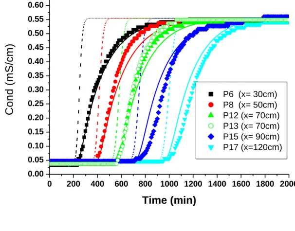
For experiment 1, electrical conductivities (EC) were measured by electrodes located at P6, 21
P8, P12, P13, P15, and P17 (see Fig. 1) at distances of 30, 50, 70, 70, 90 and 120 cm, 22
respectively, from the inlet. 23
The temporal evolution of the EC at electrodes P6, P12, P13, and P17, which are 1
representative of the EC changes in the tank, is depicted in Fig. 2. The fronts are not as sharp 2
as expected and display some tailings before reaching a constant value. The breakthrough 3
curves for the two electrodes located at the same distance (P12 and P13) from the inlet are 4
very similar, showing that the packing of the porous material was quite homogeneous. At 5
steady state conditions for all electrodes, the measured values of the EC range between 0.54 6
to 0.56 mS/cm, which is below the EC of the solution measured in the inlet reservoir (1.38 7
mS/cm). These underestimates are due to the presence of the porous medium. A linear 8
relationship between the EC in a solution with or without the presence of a given porous 9
medium was found for this kind of electrode by additional experiments. The coefficient of 10
proportionality can be estimated by comparing the EC of the injected solution and the value 11
reached in the porous material at steady state. 12
The numerical simulations were run using the parameters and initial and boundary conditions 13
described in Table 1. The arrival times were well reproduced, and the computed values 14
display a sharp front as expected (Fig. 2). However, the agreement between the measured and 15
computed EC remains quite poor. These discrepancies are assumed to be due to mixing 16
between the entering fluid and the fluid located inside the glass cylinder of the electrode. The 17
simulations also assume that mixing in this small reservoir can be considered instantaneous. 18
The solute mass balance in this reservoir is given by 19 r r C v Q(C C ) t 20
where v is the volume of water in the cylinder, Q is the flow rate through the reservoir and C r 21
is the solute concentration in the reservoir. As previously noted, since the model is linear in 22
concentration, EC can be used as a state variable and C represents the measured EC. r 23
The flow rate Q was estimated by multiplying the flow velocity in the porous medium by the 1
cross sectional area of the capture zone due to the device entrance hole. Since the glass beads 2
were filling the electrode reservoir, we assumed that the area of the capture zone coincides 3
with the hole’s area. The electrode characteristics were measured for several tested electrodes. 4
The volume of the cylinder was equal to 0.188 cm3 and the diameters of the holes ranges 5
between 0.10 and 0.12 cm. 6
The EC inside the reservoir is computed by convolution with the EC simulated by TRACES 7
as input signal, i.e. 8 t Q(t ) / v r s 0 EC (t)
EC ( ) e d 9The simulations were run with a diameter of the hole of 0.10 cm and porosity inside the 10
reservoir equal to the porosity in the porous medium. Considering mixing dynamics inside the 11
reservoir highly improves significantly the quality of the simulation results (Fig. 2). 12
13
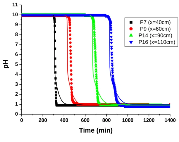
Fig. 3 shows the pH evolution during experiment 2 at the four electrodes P7, P9, P14 and P16, 14
located at 40, 60, 90 and 110 cm, respectively, from the injection (Fig. 1). Modeling of the pH 15
fronts inside the tank leads to good results without any parameter calibration (Fig. 3). 16
17
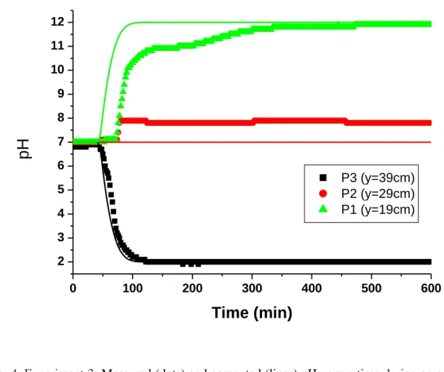
The measurements at the Eh and pH electrodes can be relevant to study the transport of 18
different solutes in porous media. Experiment 3 was aimed at studying the mixing of two 19
different fluids. Two solutions with different pH and Eh were injected in the system (see 20
Table 1). We focus on the pH values measured at 10 cm from the injection and following 21
three locations (Fig 1.): 22
- P1, located on the side in which the basic solution was injected; 23
- P2, at the middle of the tank, at the interface of both solutions; 1
- P3, positioned on the side where the acid solution was injected. 2
The changes of pH were observed simultaneously for the electrodes P1 and P3 (Fig. 4). The 3
electrode located at the interface (P2) reached a value close to neutrality, as expected. The 4
interface zone, colored in violet, is clearly visible in Fig. 5. Interestingly, the fronts do not 5
appear as sharp as those observed in experiment 2, and the pH value at the interface is not as 6
stable as the values observed at the two other electrodes. Despite the small thickness of the 7
interface, the pH electrodes we employed were able to record a pH around 7, revealing the 8
acid-base reaction between nitric acid and sodium hydroxide. 9
The simulation is in good agreement with the observed transport dynamics of the acid. The 10
tailing observed in the basic part of the tank and the pH value at the interface could not be 11
reproduced with the ADRE model. This could be due to some uncertainties in the 12
experimental conditions, such as small differences in the in-fluxes between the two inlet 13
reservoirs and/or the position of the electrode. The impact of such differences on inlet fluxes 14
on the modeling of laboratory scale scenarios has been described by Fajraoui et al. (2011) 15
through global sensitivity analyses techniques. 16
17
Electrodes of redox potential were also inserted into the porous medium during the same 18
experiment. Although the experimental conditions are not optimal for the electrodes (no redox 19
reactions), the electrodes were tested with the same solutions employed in experiment 3 20
(nitric acid and sodium hydroxide solutions), which display redox potential differences (260 21
mV/NHE for the acid solution and 730 mV/NHE for the basic solution). The results at four 22
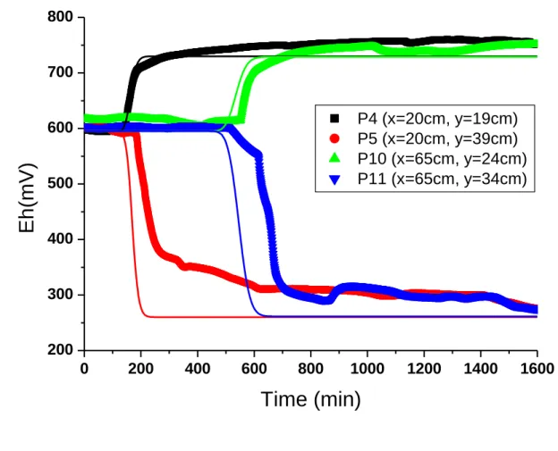
selected electrodes are presented in Fig. 6. Electrodes at P5 and P11 (resp. at P4 and P10) 23
were positioned on the side of the tank where the injection of HNO3 (resp. NaOH) at 10-2 24
mol/L was performed, at 20 and 65 cm, respectively, from the injection. 25
The changes in the Eh started approximately at the same time for the electrodes located at the 1
same distance from the inlet (P4 and P5, P10 and P11). Asymptotic values obtained in the 2
sodium hydroxide solution were close for both electrodes (258 and 264 mV/NHE) and in 3
good agreement with the value measured in the solution within the injection tank. Similar 4
results were obtained for the acid solution, and similar Eh were measured for both electrodes 5
(748 and 751 mV/NHE), which are close to the injection region. The Eh front displays 6
significant tailing effects when compared to the pH fronts. Moreover, for both pH and Eh, the 7
tailing was more significant at 0 y 29 than within other regions in the tank. 8
As expected, the simulations did not succeed in reproducing these tailings (Fig. 6). If the 9
previously mentioned uncertainties still have an effect on the results, the tailing is 10
significantly more important for the Eh than it is for pH for the same experimental conditions. 11
Two additional points can be considered to explain the behavior of Eh: (i) the design of the 12
electrodes, which did not allow the on-line measurements of the redox potential in the 13
presence of abrupt changes in time, and (ii) some additional processes, which remain 14
unknown. However, the observations were made at a considerable distance from the interface, 15
suggesting that the first assumption is the most likely. 16
17
4. Conclusions
18 19
Improved understanding of reactive transport in saturated media is a necessary step to assess 20
mathematical and numerical models. Experiments at the laboratory scale may avoid model 21
calibration, allow a good control of initial and boundary conditions and therefore provide 22
observations which are well suited for model verification. 23
New experiments in a 2D saturated porous material were presented. It was shown that 24
- 2D experimental set-ups can be used with on-line measurements of the electrical 1
conductivity and pH inside a saturated porous media. 2
- Electrodes with an internal reservoir can considerably change the apparent 3
concentration evolution due to mixing inside this reservoir, which can lead to 4
erroneous interpretation of the transport phenomena. 5
- EC can be considered as a state variable obeying the conservative transport equation. 6
Simulating evolution of pH requires solving a classical ADE, as detailed in section 7
2.3. 8
- The evolution of the redox potential displayed some tailing, probably due to the 9
characteristic time required by the electrode to obtain a stable value. Therefore, with 10
the electrodes used in this set-up, it was not possible to characterize the sharp redox 11 fronts. 12 13 14 Acknowledgement: 15
The authors gratefully acknowledge the financial support of the High Council for 16
Scientific and Technological Cooperation between France-Israel (Project Research 17
Networks Program in Water Science, Resources Management) and Prof. A. Guadagnini, 18
Politcnico di Milano for helpful discussions. 19
The described data set can be obtained by simple request. 20
21 22 23
1
5. References
2 3
André, C., Sardin, M., Vitorge, P., Faure, M-H., 1998. Analysis of breakthrough curves of 4
Np_V/ in clayey sand packed column in terms of mass transfer kinetics. J. Contam. Hydrol., 5
35, 161–173.
6
Bauer, R.D., Maloszewski, P., Zhang, Y., Meckenstock, R.U., Griebler, C., 2008. Mixing-7
controlled biodegradation in a toluene plume - Results from two-dimensional laboratory 8
experiments. J. Contam. Hydrol., 96, 150-168. 9
Burris, D.R., Hatfield, K., Wolfe, N.L., 1996. Laboratory experiments with heterogeneous 10
reactions in mixed porous media. J. Environ. Eng., 122, (8), 685-691. 11
Carrayrou, J., Hoffmann, J., Knabner, P., Kräutle, S., De Dieuleveult, C., Erhel, J., Van der 12
Lee, J., Lagneau, V., Mayer, U., MacQuarrie, K., 2010. Comparison of numerical methods for 13
simulating strongly nonlinear and heterogeneous reactive transport problems—the MoMaS 14
benchmark case. Computat. Geosci., 14, (3), 483-502. 15
Chiogna, G., Eberhardt, C., Grathwohl, P., Cirpka, O.A., Rolle, M., 2010. Evidence of 16
Compound-Dependent Hydrodynamic and Mechanical Transverse Dispersion by Multitracer 17
Laboratory Experiments. Environ. Sci. Technol., 44, (2), 688-693. 18
De Simoni, M., Carrera, J., Sanchez-Vila, X., Guadagnini, A., 2007. A procedure for the 19
solution of multicomponent reactive transport problems. Water Resour. Res., 41, 1-16. 20
Edery, Y., Scher, H., Berkowitz, B., 2009. Modeling bimolecular reactions and transport in 21
porous media. Geophys. Res. Lett., 36, L02407, doi:10.1029/2008GL036381. 22
Edery, Y., Scher, H., Berkowitz, B., 2010. Particle tracking model of bimolecular reactive 23
transport in porous media. Water Resour. Res., 46, W07524, doi:10.1029/2009WR009017. 24
Edery, Y., Guadagnini, A., Sher, H. Berkowitz, B., 2012. Reactive transport in disordered 1
media: role of fluctuations in interpretation of laboratory experiments. Adv. Water Resour., 2
doi:10.1016/j.advwatres.2011.12.008. 3
Fahs, M., Younes, A., Delay, F., 2009. On the use of large time steps with ELLAM for 4
transport with kinetic reactions over heterogeneous domains. AIChE J., 55, (5), 1121-1126. 5
Fajraoui N., Ramasomanana F., Younes A., Mara T., Ackerer P., Guadagnini A., 2011. Use of 6
Global Sensitivity Analysis and Polynomial Chaos Expansion for Interpretation of Non-7
reactive Transport Experiments in Laboratory-Scale Porous Media. Water Resour. Res., 47, 8
W02521, doi: 10.1029/2010WR009639. 9
Gramling, C.M., Harvey, C.F., Meigs, L.C., 2002. Reactive transport in porous media: A 10
comparison of model prediction with laboratory visualization. Environ. Sci. Technol., 36, 11
(11), 2508-2514. 12
Gandhi, S., Oh, B-T., Schnoor, J.L., Alvarez, P.J.J., 2002. Degradation of TCE, Cr(VI), 13
sulfate, and nitrate mixtures by granular iron in flow-through columns under different 14
microbial conditions. Water Res., 36, 1973-1982. 15
Grolimund, D., Borkovec, M., 2006. Release of colloidal particles in natural porous media by 16
monovalent and divalent cations. J. Contam. Hydrol., 87, 155-175. 17
Hoffmann J., Kräutle S., Knabner P., 2010, A parallel global-implicit 2-D solver for reactive 18
transport problems in porous media based on a reduction scheme and its application to the 19
MoMaS benchmark problem. Comput Geosci (2010) 14:421–433, doi 10.1007/s10596-009-20
9173-7 21
Hoteit, H., Ackerer, P., 2004. TRACES Transport of RadioActive Elements in Subsurface, 22
User’s guide v1.20, 70 p. 23
Jones, E.H., Smith, C.C., 2005. Non-equilibrium partitioning tracer transport in porous media: 1
2-D physical modelling and imaging using a partitioning fluorescent dye. Water Res., 39, 2
5099-5111. 3
Katz, G.E., Berkowitz, B., Guadagnini, A., Saaltink, M.W., 2010. Experimental and modeling 4
investigation of multicomponent reactive transport in porous media. J. Contam. Hydrol., 5
doi:10.1016/j.jconhyd.2009.11.002. 6
Kinzelbach, W., Schafer, W., Herzer, J., 1991. Numerical modeling of natural and enhanced 7
denitrification processes in aquifers. Water Resour. Res., 27, (6), 1123-1135. 8
Konz, M., Ackerer, P., Younes, A., Huggenberger, P., Zechner, E., 2009a. 2D stable layered 9
laboratory-scale experiments for testing density-coupled flow models. Water Resour. Res., 10
45, doi:10.1029/2008WR007118. 11
Konz, M., Ackerer, P., Huggenberger, P., Veit, C., 2009b. Comparison of light transmission 12
and reflection techniques to determine concentrations in flow tank experiments. Exp. Fluids., 13
47, 85-93. 14
Lewis, J., Sjöstrom, J., 2010. Optimizing the experimental design of soil columns in saturated 15
and unsaturated transport experiments. J. Contam. Hydrol., 115, 1-13. 16
Rolle, M., Eberhardt, C., Chiogna, G., Cirpka, O.A., Grathwohl, P., 2009. Enhancement of 17
dilution and transverse reactive mixing in porous media: Experiments and model-based 18
interpretation. J. Contam. Hydrol., 110, 130-142. 19
Saaltink, M.W., Carrera, J., Ayora, C., 2001. On the behavior of approaches to simulate 20
reactive transport. J. Contam. Hydrol., 48, 213–235. 21
Sanchez-Vila X., Fernàndez-Garcia, D., Guadagnini, A., 2010. Interpretation of column 22
experiments of transport of solutes undergoing an irreversible bimolecular reaction using a 23
continuum approximation. Water Resour. Res., 46, W12510, doi:10.1029/2010WR009539. 24
Sanford, W., Konikow, L., 1989. Simulation of calcite dissolution and porosity changes in 1
saltwater mixing zones in coastal aquifers. Water Resour. Res., 25, (4), 655-667. 2
Siegel, P., Mosé, R., Ackerer, P., Jaffre, J., 1997. Solution of the advection-diffusion equation 3
using a combination of discontinuous and mixed finite elements. Int. J. Num. Methods in 4
Fluids, 24, (6), 595-613. 5
Su, C., Puls, R.W., 2004. Significance of Iron (II,III) Hydroxycarbonate Green Rust in 6
Arsenic Remediation Using Zerovalent Iron in Laboratory Column Tests. Environ. Sci. 7
Technol., 38, 5224-5231. 8
Steefel, C., DePaolo, D., Lichtner, P., 2005. Reactive transport modeling: An essential tool 9
and a new research approach for the Earth sciences. Earth Planet. Sc. Lett., 240, (3-4), 539-10
558. 11
Van der Lee, J., De Windt, L., Lagneau, V., Goblet, P., 2003. Module-oriented modeling of 12
reactive transport with HYTEC. Comp. Geosci., 29, 265-275. 13
Walter, A.L., Frind, E.O., Blowes, D.W., Ptacek, C.J., Molson, J.W., 1994. Modeling of 14
multicomponent reactive transport in groundwater 1. Model development and evaluation. 15
Water Resour. Res., 30, (11), 3137-3148. 16
Yeh, G.T., Tripathi, V.S., 1991. Model for simulating transport of reactive multispecies 17
components — model development and demonstration. Water Resour. Res., 27, (12), 3075-18
3094. 19
Younes, A., Ackerer, P., Delay, F., 2010. Mixed finite element for solving diffusion-type 20
equations. Rev. Geophys., 48, RG1004, doi:10.1029/2008RG000277. 21
Zinn, B., Meigs, L.C., Harvey, C.F., Haggerty, R., Peplinski, W.J., Von Schwerin, C.F., 2004. 22
Experimental Visualization of Solute Transport and Mass Transfer Processes in Two-23
Dimensional Conductivity Fields with Connected Regions of High Conductivity. Environ. 1 Sci. Technol., 38, 3916-3926. 2 3 4 5 6
Figure Captions
1 2
Fig. 1: (a) Experimental set-up and (b) top-view of the set-up with the potential position of the 3
different electrodes (open circle). 4
5
Fig. 2. Experiment 1: Measured (dots) and computed (lines) EC versus time during injection 6
of KCl solution, without “mixing” effects (dashed lines) and with “mixing” effects 7
(continuous lines). 8
9
Fig. 3. Experiment 2: Measured (dots) and computed (lines) pH versus time during injection 10
of nitric acid solution. 11
12
Fig. 4. Experiment 3: Measured (dots) and computed (lines) pH versus time during an acido-13
basic reactive transport. 14
15
Fig. 5. Experiment 3: Electrodes monitoring during reactive transport: photograph showing 16
the interface zone between red acid solution and blue sodium hydroxide solution. 17
18
Fig. 6. Experiment 3: Measured (dots) and computed (lines) Eh versus time during a 19
simultaneously injection of nitric acid and sodium hydroxide solutions. 20
21 22
Table 1: Parameters for the simulations 1 Domain size 1.52 x 0.58 m Hydraulic conductivity: K 3.34×10⁻³ m/s Effective porosity: 0.375 Longitudinal dispersivity: L 0.0008 m Transverse dispersivity: T 0.00008 m Molecular diffusion D : m 1.0×10-09 m2/s Experiment 1.
Inflow boundary condition H0.25 m
Outflow boundary condition 6
L
q 7.60 x10 m / s Initial condition
0
C 0.04 mS/ cm(Cond) Upstream boundary condition
L
C 0.5546 mS/ cm(Cond)
Experiment 2.
Inflow boundary condition H0.25 m
Outflow boundary condition 6
L
q 7.33 x10 m / s Initial condition
0
C 10(pH) Upstream boundary condition
L
C 1(pH)
Experiment 3.
Inflow boundary condition H0.25 m
Outflow boundary condition 6
L
q 7.63 x10 m / s Initial condition
0
C 7 (pH)
Upstream boundary condition L
L C (0.0 y 0.29) 12 (pH) C (0.29 y 0.58) 2 (pH) Initial condition 0 C 595mV (Eh)
Upstream boundary condition
L L C 0.0 y 0.29 730 mV (Eh / NHE) C 0.29 y 0.58 260 mV (Eh / NHE) 2 3 41 2 (a) 3 4 (b) 5
Fig. 1: (a) Experimental set-up and (b) top-view of the set-up with the potential position of
6
the different electrodes (open circle). 7
8 9 10 11
1
Fig. 2. Experiment 1: Measured (dots) and computed (lines) EC versus time during injection 2
of KCl solution, without “mixing” effects (dashed lines) and with “mixing” effects 3 (continuous lines). 4 0 200 400 600 800 1000 1200 1400 1600 1800 2000 0.00 0.05 0.10 0.15 0.20 0.25 0.30 0.35 0.40 0.45 0.50 0.55 0.60
C
o
n
d
(
m
S
/c
m
)
Time (min)
P6 (x= 30cm) P8 (x= 50cm) P12 (x= 70cm) P13 (x= 70cm) P15 (x= 90cm) P17 (x=120cm)1
Fig. 3. Experiment 2: Measured (dots) and computed (lines) pH versus time during injection 2
of nitric acid solution. 3 4 5 6 7 0 200 400 600 800 1000 1200 1400 0 1 2 3 4 5 6 7 8 9 10 11
pH
Time (min)
P7 (x=40cm) P9 (x=60cm) P14 (x=90cm) P16 (x=110cm)1
2
Fig. 4. Experiment 3: Measured (dots) and computed (lines) pH versus time during an acido-3
basic reactive transport. 4
5 6 0 100 200 300 400 500 600 2 3 4 5 6 7 8 9 10 11 12
pH
Time (min)
P3 (y=39cm) P2 (y=29cm) P1 (y=19cm)Fig. 5. Experiment 3: Electrodes monitoring during reactive transport: photograph showing 1
the interface zone between red acid solution and blue sodium hydroxide solution. 2
3 4 5 6
1 2
3
Fig. 6. Experiment 3: Measured (dots) and computed (lines) Eh versus time during a 4
simultaneously injection of nitric acid and sodium hydroxide solutions. 5 6 7 8 0 200 400 600 800 1000 1200 1400 1600 200 300 400 500 600 700 800