Generalized Sub‐Gaussian Processes: Theory and Application to Hydrogeological and Geochemical Data

HAL Id: hal-03010938

https://hal.archives-ouvertes.fr/hal-03010938

Submitted on 17 Nov 2020

HAL is a multi-disciplinary open access

archive for the deposit and dissemination of sci-entific research documents, whether they are pub-lished or not. The documents may come from teaching and research institutions in France or abroad, or from public or private research centers.

L’archive ouverte pluridisciplinaire HAL, est destinée au dépôt et à la diffusion de documents scientifiques de niveau recherche, publiés ou non, émanant des établissements d’enseignement et de recherche français ou étrangers, des laboratoires publics ou privés.

Martina Siena, Alberto Guadagnini, Arnaud Bouissonnié, Philippe Ackerer,

Damien Daval, Monica Riva

To cite this version:

Martina Siena, Alberto Guadagnini, Arnaud Bouissonnié, Philippe Ackerer, Damien Daval, et al.. Generalized Sub-Gaussian Processes: Theory and Application to Hydrogeological and Geochemical Data. Water Resources Research, American Geophysical Union, 2020, 56 (8), �10.1029/2020wr027436�. �hal-03010938�

Generalized Sub-Gaussian processes: theory and application to hydrogeological and

1

geochemical data

2

Martina Siena1_{, Alberto Guadagnini}1_{, Arnaud Bouissonnié}2_{, Philippe Ackerer}2_{, Damien}

3

Daval2_{, Monica Riva}1

4

1_{Dipartimento di Ingegneria Civile e Ambientale, Politecnico di Milano, Piazza L. Da Vinci 32,} 5

20133 Milano, Italy

6

2_{Université de Strasbourg-CNRS ENGEES/EOST, Laboratoire d’Hydrologie et de Géochimie de} 7

Strasbourg, Strasbourg, France

8

Corresponding author: Martina Siena ([email protected])

9

Key Points: 10

 We develop the theoretical formulation of the Generalized Sub-Gaussian (GSG) model

11

for a general distributional form of the subordinator.

12

 The GSG formulations tested on laboratory- and field-scale data effectively capture the

13

observed scale dependence of increments’ statistics.

14

 Our formulations can improve flexibility and accuracy of the GSG model, supporting its

15

applicability to a wide range of data.

16 17

Abstract 18

We start from the well-documented scale dependence displayed by the probability distribution and

19

associated statistical moments of a variety of hydrogeological and soil science variables and their

20

spatial or temporal increments. These features can be captured by a Generalized Sub-Gaussian

21

(GSG) model, according to which a given variable, Y, is subordinated to a (typically spatially

22

correlated) Gaussian random field, G, through a subordinator, U. This study extends the theoretical

23

framework originally proposed by Riva et al. (2015a) to include the possibility of selecting a

24

general form of the subordinator distribution, thus enhancing the flexibility of the GSG framework

25

for data interpretation and modeling. Analytical expressions for the GSG process associated with

26

(i) lognormal, (ii) Pareto, and (iii) Gamma subordinator distributions are then derived. We

27

demonstrate the ability of the GSG modeling framework to capture the way key features of the

28

statistics associated with two datasets transitiona cross scales. The latter correspond to variables

29

which are typical of a geochemical and a hydrogeological setting, i.e., (i) data characterizing the

30

micrometer-scale surface roughness of a crystal of calcite, collected within a laboratory-scale

31

setting under given environmental conditions inducing mineral dissolution; and (ii) a vertical

32

distribution of decimeter-scale porosity data, collected along a deep km-scale borehole within a

33

sandstone formation and typically used in hydrogeological and geophysical characterization of

34

aquifer systems.The theoretical developments and the successful applications of the approach we

35

propose provide a unique framework within which one can interpret a broad range of scaling

36

behaviors displayed by a variety of Earth and environmental variables in various scenarios.

37

Plain Language Summary 38

Characterization of hydrogeological and geochemical systems aims at assessing the heterogeneity

39

and scale dependency exhibited by their attributes and the associated key statistics. It has been

40

shown that complex scaling features documented for the statistics of a wide range of Earth,

41

environmental (and several other) variables and their spatial/temporal increments can be captured

42

through a Generalized Sub-Gaussian (GSG) model. The latter relies on the subordination of a

43

Gaussian random field through a subordinator. This study extends the theoretical framework

44

originally proposed for the GSG model to include multiple choices of the subordinator distribution.

45

We provide the theoretical formulation and discuss the main features of the GSG model resulting

46

from (i) a general form of the subordinator and (ii) three selected distributional forms. We show

the effectiveness of the GSG modeling framework for the interpretation of real data encompassing

48

a considerably wide range of scales by analyzing (i) a set of surface topography (roughness) data

49

collected on a calcite sample in a laboratory-scale geochemical setting; and (ii) a field-scale

50

distribution of porosity data, collected along a deep borehole within a sandstone formation.

51

1 Introduction 52

Geostatistical models adopted for the interpretation of key features of spatial heterogeneity

53

of quantities related to subsurface flow and transport processes consider available observations of

54

a variable of interest as samples from a random field with a given distribution. Analyses of a wide

55

collection of datasets of hydrogeological attributes, including, e.g., (log) hydraulic conductivity

56

and permeability (Liu & Molz, 1997; Meerschaert et al., 2004; Painter, 2001; Painter, 1996, Riva

57

et al., 2013a, 2013b; Siena et al., 2012, 2019), electrical resistivity (Painter, 2001), and neutron

58

porosity (Guadagnini et al., 2015; Riva et al., 2015a) observations, clearly document the

59

occurrence of distinct non-Gaussian features characterizing their distributions. Notably, it has been

60

shown that spatial increments, Y( )s Y(x s ) Y( )x , evaluated over separation distance (or lag) 61

s (x being a position vector) of a given quantity Y are characterized by distributions displaying 62

peaks that become sharper and tails that tend to become heavier with decreasing lag. A similar

63

behavior, corresponding to distributions transitioning from heavy tailed at small lags to

seemingly-64

Gaussian at increased lags, is documented by analyses of a variety of spatial and/or temporal

65

increments of environmental data, including sediment transport processes (e.g., Ganti et al., 2009)

66

and fully developed turbulence (Boffetta et al., 2008) as well as datasets of Earth, environmental

67

and several other variables (see Neuman et al., 2013 and references therein). Such a scale

68

dependence is directly imprinted to the associated (statistical) moments of increment distributions.

69

All of these evidences suggest that modeling the (spatially correlated) variability of Y

70

through a Gaussian model is not generally warranted. With specific reference to the spatial

71

variability of hydrogeologic quantities, a number of studies evidence that the heterogeneity of

72

natural aquifers is generally more complex than what can be captured through a Gaussian model

73

(e.g., among others, with reference to hydraulic conductivity, Gómez-Hernández & Wen, 1998;

74

Haslauer et al., 2012; Mariethoz et al., 2010; Xu & Gómez-Hernández, 2015 and references

75

therein).

In this context, it is also noted that attributes/properties of porous media that at some scale

77

can be considered as composed by distinct facies/regions, each corresponding to a given material

78

characterized by an internal degree of heterogeneity, could be represented through multi-modal

79

distributions (see, e.g., Desbarats, 1990; Lu & Zhang, 2002; Rubin, 1995; Russo, 2002, 2010;

80

Winter et al., 2003 and references therein). The latter are representative of a conceptual (and

81

mathematical) model that views the otherwise composite nature of the system as a unique

82

continuum at the given scale of observation, natural variability within each region being

83

characterized by a statistical behavior of the kind described above.

84

Riva et al. (2015a, b) show that the above illustrated scale-dependent behavior of the

85

probability density function (pdf) of Y can be captured through a Generalized Sub-Gaussian

86

(GSG) model. This theoretical framework relies on the idea that the spatial random field

87

( ) ( )

Y x    Y Y x , Y  and ( )Y x being respectively the ensemble mean and a local zero-mean

88

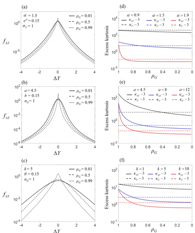
fluctuation, can be interpreted through the following model

89

 

   

Y x U x G x . (1)

90

Here, G x is a zero-mean, Gaussian random field and

 

U x is a so-called subordinator,

 

91

independent of G, consisting of statistically independent identically distributed (iid) non-negative

92

random variables. The underlying Gaussian random field generally (but not necessarily) displays

93

a multi-scale nature which can be captured, for example, through a geostatistical description based

94

on a Truncated Power Variogram model (e.g., Di Federico & Neuman, 1997; Neuman & Di

95

Federico, 2003).

96

As opposed to mathematical models based on multifractals (e.g., Boffetta et al., 2008; Frisch,

97

2016; Lovejoy & Schertzer, 1995; Mandelbrot, 1974; Monin & Yaglom, 1975; Veneziano et al.,

98

2006) or fractional Laplace approaches (e.g., Kozubowski et al., 2006; Kozubowski et al., 2013;

99

Meerschaert et al., 2004), which have been employed to mimic the above-mentioned pattern of

100

increment frequency distributions, the GSG model enables one to represent jointly within a unique

101

theoretical framework the documented behavior (as described by probability distributions and/or

102

moments) of a quantity and its incremental values.

103

Riva et al. (2015a) provide the first analytical formulation of the GSG model, illustrating

104

that the characteristic scaling behavior of the increments results from the decay of the correlation

105

function of the underlying Gaussian random field with increasing lag. Riva et al. (2015b) illustrate

an approach for the generation of unconditional random realizations of statistically isotropic or

107

anisotropic GSG fields in multiple dimensions. Panzeri et al. (2016) develop an algorithm for the

108

generation of GSG fields conditional to a given set of data. Siena et al. (2019) rely on the GSG

109

model for the interpretation of the spatial variability of a set of air permeability data collected

110

along a core of limestone. Guadagnini et al. (2018) present a 9-step procedure for the detection of

111

GSG signatures in a given dataset. Notably, theoretical developments and applications to date rest

112

solely on a lognormal distribution of U characterized by a single parameter, thus limiting the range

113

of possible applications of the GSG model.

114

The present study focuses on a generalization of the GSG framework by extending the

115

formulation of Riva et al. (2015a) to include a generic subordinator. This enables us to enhance

116

the flexibility of the model for data interpretation and modeling by taking into account specific

117

features exhibited by the way statistics of a given dataset transition across scales. We then

118

demonstrate the applicability of the general theoretical framework by considering a (i)

two-119

parameter lognormal; (ii) Pareto; and (iii) Gamma distributional form of U and developing the

120

ensuing analytical expressions for the GSG process. We analyze in this context two datasets

121

associated with differing processes and observation scales. The first application includes direct

122

observations of µm-scale surface topography (or roughness) of mm-scale calcite crystals resulting

123

from induced mineral dissolution. Calcite is a common mineral in the Earth’s crust and is

124

characterized by significant dynamics of its surface, depending on environmental conditions (e.g.

125

Fischer et al., 2012; Jordan & Rammensee, 1998; Noiriel et al., 2009, 2020). Acquisition of the

126

type of data we consider is subject to increased interest to characterize micro-scale geochemical

127

processes deriving from interactions taking place at fluid-rock interfaces (e.g., Bouissonnié et al.,

128

2018; Pollet-Villard et al., 2016a, b and references therein). While the possibility of acquiring

129

these direct observations is continuously enhanced through the use of modern atomic force

130

microscopy and vertical scanning interferometry, statistical analyses of available datasets are still

131

limited to standard variography (Pollet-Vilard et al., 2016a). As an additional test-bed, we analyze

132

a vertical profile of neutron porosity data, collected along a deep borehole in a sandstone formation

133

and encompassing a vertical depth of about 1 km at a 15-cm resolution (Dashtian et al., 2011). As

134

these types of data are routinely available in (hydro)geological and geophysical subsurface

135

exploration, they constitute a remarkable dataset to assess the applicability of our statistical scaling

136

framework at such scales.

The work is structured as follows. Section 2 illustrates the key features of the GSG model

138

and describes a moment-based method of inference of model parameters. The detailed original

139

analytical formulation of the GSG model associated with a generic subordinator and the ensuing

140

derivations for the three subordinators here considered are provided in Appendix A and B,

141

respectively. In Section 3 we compare the performance of these three alternative GSG models for

142

the interpretation of the two datasets illustrated above. Concluding remarks are provided in Section

143

4.

144

2 Generalized Sub-Gaussian model 145

2.1 Theoretical framework

146

Zero-mean fluctuations, Y, at two spatial locations, x₁ and x₂, can be expressed as

147

 

i

   

i i i i i

Y x U x G x  Y U G, with i = 1, 2. (2)

148

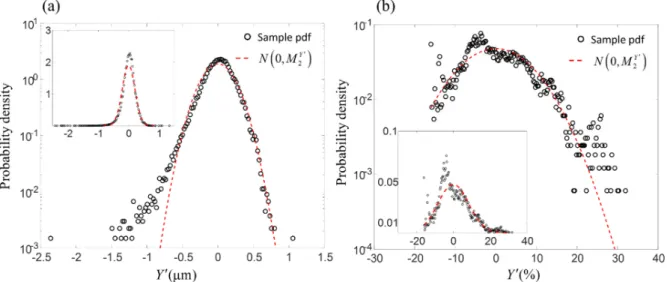
The bivariate pdf of Y₁ and Y₂ is (Riva et al., 2015a)

149





   

1 2 1 2 1 2 1 2 2 1 , 1 2 1 2 1 2 2 1 0 0 , , Y Y U U G G y y du du f y y f u f u f u u u u           _{ }  

 

, (3) 150 where

 

i U i

f u is the pdf of Ui and fG G_{1 2} is the bivariate pdf of G1 and G2, given by

151   2 2 1 2 1 2 2 2 2 2 1 2 1 2 1 2 1 ₂ 2 1 1 2 2 2 1 2 , 2 1 G G G y y y y u u u u G G G G y y e f u u             _   _              , (4) 152 where, 2 G

 is the variance of G and _G is the correlation coefficient between G₁ and G₂, which

153

typically decreases as the separation distance (or lag)

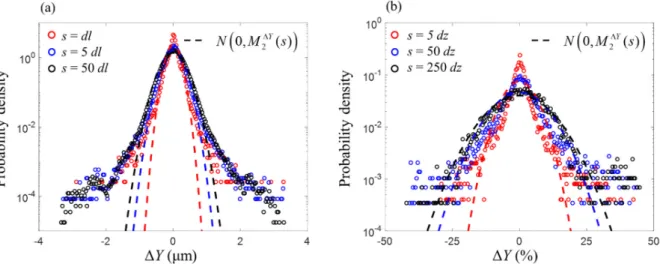
s

 

x x

_{1 2} increases. Starting from Riva et

154

al. (2015a), who developed the analytical framework for the specific case of a single-parameter

155

lognormal subordinator, we provide in Appendix A an original theoretical formulation of the GSG

156

model considering a generic distributional form of U. It is worth noting that, regardless the

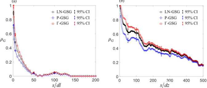
157

distributional form of U, the variogram of Y' is always characterized by a nugget effect (see Eq.

158

A14), rendered by the product of the variance of G and the variance of U. This result implies that

159

nugget effects, which are typically considered to appear due to variability of Y' at scales smaller

160

than the sampling interval and/or to measurement errors, may in fact be (at least in part) considered

161

as a symptom of non-Gaussianity of the type embedded in the GSG theoretical framework.

The general framework introduced in Appendix A encompasses multiple possible

163

formulations of the GSG model: in this context, we evaluate three possible alternative models for

164

U, corresponding to a lognormal, Pareto, or Gamma distribution. Each of these models is

165

characterized by NP = 2 parameters, respectively controlling the shape (shape parameter) and the 166

spreading (scale parameter) of the pdfs of the ensuing GSG formulation for Y'. Hereinafter, we

167

denote the latter as LN-GSG, P-GSG, and Γ-GSG for the lognormal, Pareto, and Gamma

168

subordinator, respectively. The theoretical formulation of each of these GSG models is provided

169

in Appendix B.

170

Equations (A7) indicate that the pdfs f_Y of incremental values (Y) corresponding to

171

differing lags depend on (i) 2

G

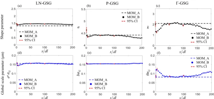
 and the NP parameters of U; and (ii) _G. While the former 172

parameters are constant for all lags, the correlation function of G is lag-dependent, thus imprinting

173

a scaling behavior, i.e., an intrinsic variability with lag, to the shape of the pdf of incremental

174

values of Y', independent of the GSG model considered. This feature is clearly illustrated in

175

Figures 1a-c, where we depict f_Y for selected values of the three GSG model parameters

176

(analytical expressions being collected in Eq. (B8)) and three values of _G corresponding to short,

177

intermediate and large lags. The pattern associated with the behavior of peaks and tails of the pdfs

178

of Y' and Y can be described quantitatively by analyzing their standardized kurtosis,



_Y (see

179

Eq. (A6)) and



_Y (see Eq. (A11)), respectively, deviations from Gaussianity being clearly

180

revealed by the excess kurtosis,



_Y3 and



_Y3. As these quantities increase, the peak of the

181

pdf of Y' or Y grows sharper and the associated tails become heavier. Figures 1d-f depict the

182

excess kurtosis of Y', as well as of Y, as a function of _G for selected values of the shape

183

parameter



(for the LN-GSG model, Fig. 1d), a (for the P-GSG model, Fig. 1e), and k (for the Γ-184

GSG model, Fig. 1f). Inspection of these figures, together with Eqs. (B7) and (B11), suggests that

185

for all GSG models (i)



_Y'3 and



_Y3 do not depend on the scale parameter of the subordinator

186

and on the variance of G; (ii) for a given value of _G,



_Y3 and



_Y3 increase as the shape

187

parameter of U decreases; (iii) for a given value of the shape parameter,



_Y3 increases as _G

188

increases (or, equivalently, as lag decreases), i.e., the pdfs of Y transition with lag. One can note

189

that, in all cases,



_Y 3 exceeds zero by a significant margin at small lags (i.e., as_G  ), even 1

for the largest values of the shape parameter of U considered. With reference to the LN-GSG

191

model, Figure 1d and Eqs. (B7) and (B11) highlight that there is a threshold value of the shape

192

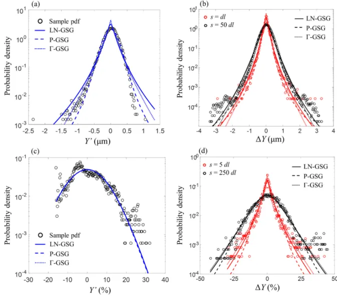
parameter, corresponding to T  2 ln 3 0.95 , such that (i) for   T , the pdfs of Y are

193

characterized by lower peaks and lighter tails than those of Y at all lags; while (ii) for   _T,

194

3

Y



  is higher/lower than



Y'3 at small/large lags (see also Riva et al., 2015a). An analogous

195

behavior is exhibited by the results associated with the Γ-GSG model (Fig. 1f), the threshold value,

196

T

k , of the shape parameter being equal to 1.0. Otherwise, one can demonstrate analytically (see

197

also Fig. 1e) that



_Y 3 is always larger than



_Y3 at small lags for the P-GSG model,

198

regardless the value of the shape parameter a. Besides, the range of values of _G for which (

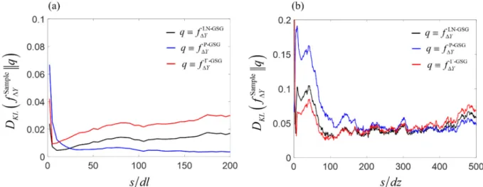
199

3

Y



  ) > (



Y'3) (i.e., the range of lags where the pdfs of the increments display sharper peaks

200

and heavier tails than the pdf of Y) tends to increase as a decreases.

201

2.2 Parameter estimation methods

202

The Method of Moment (MOM) is a straightforward way to infer model parameters from a

203

dataset. Here, we illustrate two approaches to estimate model parameters through MOM. These

204

are respectively based on (i) sample statistics of the parent variable (Method A) and (ii) sample

205

statistics of both the parent variable and the incremental data at multiple lags (Method B). Sections

206

2.2.1 and 2.2.2 examine merits and drawbacks of these methods.

207

2.2.1 Parameter estimation Method A

208

Method A (henceforth denoted as MOM_A) relies on the marginal frequency distribution

209

and associated moments of Y'. Estimates of GSG model parameters are obtained by replacing

210

2

Y and Y4 in Eqs. (A3) and (A6) with their sample counterparts, _M2Y _and 4

Y

M , inferred

211

from data. The shape parameter of U for the LN-GSG, P-GSG, and Γ-GSG models can be

212

estimated by making use of Eq. (B7) as

 

 





2 4 2 ' 2 4 2 ' 2 for LN-GSG fo , r P-GSG for , with 2 ( 2) , with 4 ( G w - SG 4) 3 4 6 1 ith 0 1 Y Y e M a a a a M k k k k 

_

   _   _  _     _    _    (5) 214

Then, by making use of Eq. (B5), one can estimate the product between _G and the scale

215

parameter of U (e.g., e, b, and , for LN-GSG, P- GSG and Γ-GSG model, respectively) as

216  2 2 2 2 2 2 Y G M e e     _  for LN-GSG, (6) 217 2 2 2 2 Y G a b M a  _   _{for P-GSG, (7)} 218





2 2 2 1 Y G M k k      for Γ-GSG. (8) 219

It is noted that the analytical expressions of the marginal pdf (as well as its statistical

220

moments) of Y for all GSG models are characterized by the scale parameter of the subordinator

221

being always coupled with the scale parameter, _G, of the underlying Gaussian process (see Eqs.

222

(B4) - (B6)). It then follows that the set of Eqs.(5)-(8) fully determines f_Y

 

y , i.e., it is not

223

necessary to estimate_G and the scale parameter of U independently to determine f_Y

 

y .As an

224

additional remark, it is noted that one cannot estimate _G with the methodology here implemented.

225

As such, its application, while straightforward, does not allow ascertaining the degree of spatial

226

correlation of the random field Y.

227

2.2.2 Parameter estimation Method B

228

Method B (henceforth denoted as MOM_B) yields estimates of GSG model parameters by

229

relying jointly on sample statistics of Y and Y. For any given lag, one replaces Y2 , Y2

230

and Y4 in Eqs. (A3), (A8), and (A9) by their sample counterparts _M2Y_, 2 Y M _{, and} 4 Y M  _, 231

respectively. Making use of Eqs. (B5), (B9) and (B11), the resulting systems of equations are

   





      2 2 2 2 2 2 2 ' 2 2 2 2 ' ₂ 2 2 2 2 4 2 ₂ 2 2 2 1 3 1 2 1 1 2 Y G Y G Y Y Y G M = e e M = M _e e e M e M                       _      _{    }     _ _   _{    }    for LN-GSG, (9) 233





' 2 2 2 2 ' 2 2 2 2 4 2 2 2 2 2 ( 2) 1 2 ( 1) 4 1 2 1 1 2 ( 4) ( 1)( 3) ( 2) ( 2) ( 1) 3 Y G Y G Y Y G G G Y a M = b a a a M = M a a M a a a a a a a M            _    _  _          _{   }      _{        }  for P-GSG, (10) 234





















2 2 2 2 2 2 4 2 2 2 1 1 2 1 1 2 2 1 3 1 1 Y G Y G Y Y G G Y G M = k k M ₌ k M k k k k k M k M k k k                    _     _{   }          _{   }  for Γ-GSG. (11) 235

Equations (9)-(11) allow estimating all parameters characterizing the joint pdf of Y, i.e.,

236

(i) the product of the scale parameters of G and U, (ii) the shape parameter of U, and (iii) the

237

correlation coefficient



_G, which enables us to diagnose the dependence on lag of increment

238

statistics. We further note that relying on the joint use of Y and Y data is recommended because

239

it leads to an (often considerably) augmented set of data upon which sample moments are

240

evaluated, thus improving the accuracy of the estimates. This approach yields a set of three

241

parameter estimates for each investigated lag. Riva et al. (2015a) document that MOM_B provides

242

results of similar quality to those one could obtain upon relying on parameter estimation through

243

analyzing incremental data at various lags via Maximum Likelihood (ML). This element, together

244

with the high computational demand associated with ML, leads us to rely on MOM_B for the

245

purpose of our analyses.

According to our theoretical framework (see Section 2.1), we expect that values of the shape

247

parameter and of the product between the scale parameters of U and G remain (approximately)

248

constant with lag. It then follows that an additional benefit of relying on MOM_B, as opposed to

249

MOM_A, is that it enables one to assess the consistency of the parameter estimation results with

250

these theoretical requirements. As already noted for the pdf of Y, the pdf of Y (as well as its

251

statistical moments) for all GSG models is also characterized by the scale parameter of U being

252

always coupled with _G (see Eqs. (B8) - (B10)). Therefore, the inability to provide unique

253

estimates of the scale parameters of U and G (while only their product is estimated) does not

254

hamper the use of the results of the analysis for further applications, typically involving

255

generations of a collection of realizations of a given random field to be employed in the context of

256

studies on flow and transport processes in a Monte Carlo framework.

257

3 Application to laboratory- and field- scale datasets 258

The three alternative GSG models illustrated in Section 2 and in Appendix B are here

259

considered for the characterization of the spatial variability of two datasets. These are selected to

260

represent two differing observation scales, i.e., a laboratory- and a field- scale setting. Both

261

systems are characterized by the availability of a considerable amount of observations, which is

262

achievable with modern measurement techniques, and are therefore well suited for the analysis.

263

3.1 Micrometer-scale topography of a millimeter-scale calcite sample resulting from

264

mineral dissolution

265

The first dataset we consider (hereinafter denoted as Dataset 1) comprises direct observations

266

of surface topography collected on a (104) calcite cleavage plan. While calcite is the main

rock-267

forming mineral of limestones and has a key role in a variety of geological and biological systems,

268

its surface is characterized by remarkable dynamics when put in contact with aqueous fluid, which

269

are still not completely characterized, the (104) surface plane being very common in natural

270

settings. The sample consisted of a ~5mm-sized single crystal of calcite polished through a

multi-271

step abrasive sequence. The initial arithmetic roughness of the surface was on the order of 50 nm.

272

The sample was introduced in a mixed-flow reactor set-up. The crystal was subject to reaction for

273

8 days at room temperature and at a saturation index with respect to calcite of 0.8, corresponding

274

to conditions where dissolution occurs while the nucleation of etch pits is thermodynamically

impossible. Measurements of surface topography, ( , )x y being spatial coordinates in the horizontal

276

plane, are collected by means of a vertical scanning interferometer (Zygo NewView 7300) with a

277

vertical resolution of 3 nm, on a two-dimensional grid of N1 = 250×250 = 62500 cells, with lateral 278

resolution dl = 2.2 μm. Additional details of the experimental set-up and procedure are offered in

279

Bouissonnié et al. (2018). The surface is characterized by a slight curvature, resulting from the

280

preliminary polishing of the sample. Mean-removed topography data, Y, have been obtained by

281

subtracting the best-fitting quadratic surface from the measurements. Figure 2a depicts the spatial

282

distribution of Y, the sample standard deviation being equal to ₂Y

M   0.21 μm.

283

3.2 Field-scale neutron porosity data

284

Dataset 2 is a collection of neutron porosity data sampled from a (km-scale) deep vertical

285

borehole in southwestern Iran. The data are part of a wider dataset comprising multiple wells, some

286

of which have been recently analyzed by Dashtian et al. (2011), Riva et al. (2015a), and

287

Guadagnini et al. (2015). The borehole considered here is drilled in the Ahwaz field (see Dashtian

288

et al., 2011), where oil and natural gas are produced from a sandstone formation. A large number

289

(N2 = 6949) of neutron porosity data collected at a uniform distance of dz = 15 cm is available. 290

The one-dimensional profile of mean-removed porosity data is depicted in Fig. 2b, the associated

291

sample standard deviation being equal to _M2Y _8.35%_.

292

3.3 Results and discussion

293

Figures 3a and 3b depict sample pdfs of Y' for Dataset 1 and 2, respectively. Depictions are

294

provided in linear and semi-logarithmic scales for ease of analysis. A slight bimodality and

295

asymmetry are exhibited by the pdf of porosity observations in Dataset 2, the pdf of surface

296

topography (Dataset 1) being left-skewed. A qualitative comparison (based on visual inspection)

297

between each of these sample pdfs and a normal distribution with the corresponding variance, _M2Y

298

, (also included in the figures) suggests deviation from Gaussianity for both variables. This 299

qualitative result is also confirmed quantitatively by the outcomes of formal (Shapiro-Wilk,

300

Kolmogorov-Smirnov, and Anderson-Darling) tests performed on randomly-sampled subsets of

301

data, which reject the Gaussian model at a significance level of 0.05 for both datasets.

We compute sample statistics of incremental data, Y, evaluated (i) along all directions in

303

the x-y plane for Dataset 1 and (ii) along the z axis for Dataset 2. The pdfs of Y at three diverse

304

lags (s = 1, 5, and 50 dl for Dataset 1; and s = 5, 50, and 250 dz for Dataset 2) are depicted in Figs.

305

4a and 4b, respectively. As a term of comparison, corresponding normal distributions with the

306

same variance are juxtaposed to the increment pdfs. These results illustrate that sample pdfs of

307

increments (i) exhibit the characteristic scale dependence mentioned in Section 1; and (ii)

308

progressively tend to distributions with lower peaks and lighter tails, resembling the Gaussian

309

distribution as lag increases, this feature being particularly evident for Dataset 2.

310

Figures 5a and 5b depict the dependence of sample values of



_Y 3 on lag for Dataset 1

311

and Dataset 2, respectively, dashed horizontal lines denoting values of excess kurtosis of the parent

312

variable Y. For both sets, incremental data excess kurtosis is significantly larger than zero at small

313

lags. Excess kurtosis (EK) of (omnidirectional) incremental data associated with Dataset 1

314

decreases rapidly as lag increases and tends to attain a quite stable value of ≈ 3.5 at large lags.

315

Otherwise, values of EK for Dataset 2 tend to consistently decrease across the whole range of lags

316

considered, attaining values smaller than 1 (i.e., approaching a Gaussian distribution, consistent

317

with the qualitative result depicted in Fig. 4b) from s = 400 dz.

318

To provide an appraisal of the accuracy associated with the sample estimates of EK, we apply

319

a standard bootstrapping technique (Efron, 1992) to each set of incremental data. This procedure

320

relies on sampling (with replacement) from a collection of Y data related to a given lag a total

321

of m (here we set m = 10,000) sets, each characterized by the same number of elements of the

322

original collection of Y. The same procedure is then repeated for all lags considered. Figures 5a

323

and 5b depict the 95%-confidence intervals, CI, associated with the estimates of EK at four

324

representative lags. Uncertainties associated with EK estimates are (in general) negligible.

325

Threfore, we consider the observed overall decrease of EK with the lag to be significant for both

326

datasets. We note that



_Y 3 >



_Y3 at small lags for Dataset 1 (Fig. 5a), implying that

327

frequency distributions of Y exhibit sharper peaks and heavier tails than does that of Y, whereas

328

the opposite behavior is documented at large lags. Otherwise,



_Y3 >



_Y3 over the whole

329

range of lags considered for Dataset 2 (Fig. 5b). Considering the type of analyses documented in

330

Figs. 1d-f, the behavior observed for both datasets is consistent with our theoretical models for (i)

331

0.95 < α < 2 in the case of LN-GSG; (ii) a > 4 for P-GSG, and (iii) k > 1 for Γ-GSG.

Estimates of (i) the shape parameter and (ii) the product of the scale parameters of U and G

333

(henceforth denoted only as global scale parameter for conciseness) obtained via MOM_A and

334

MOM_B for each GSG model formulation are depicted in Fig. 6 (Dataset 1) and Fig. 7 (Dataset

335

2) as a function of normalized lag. These results are complemented by Table 1 where we list

336

parameter estimates obtained via MOM_A, together with mean and coefficient of variation (cv)

337

evaluated over all lags of MOM_B estimates, obtained for all GSG model formulations and both

338

datasets.

339

Considering Dataset 1, results obtained via MOM_B for LN-GSG (i.e.,



in Fig. 6a and

340

e_G in Fig. 6d) and P-GSG (i.e., a in Fig. 6b and b



_G in Fig. 6e) do not vary appreciably with

341

lag (cv ≈ 2-3%), consistent with our theoretical framework. Otherwise, MOM_B estimates of k

342

and



_G (Figs. 6c and 6f, respectively) associated with Γ-GSG are characterized by stronger

343

oscillations around an average value, as indicated by larger values of the corresponding coefficient

344

of variation, as compared to the other models. Nevertheless, values of cv range between 18% (for

345

the shape parameter) and 22% (for the global scale parameter), which (also in view of ubiquitously

346

present experimental uncertainties) can still be considered as a good approximation of the

347

constraints associated with theoretical requirements. Figure 6 and Table 1 also document that

348

MOM_A estimates are consistent with their counterparts obtained via MOM_B for all models.

349

Results for Dataset 2 (Fig. 7) obtained through MOM_B generally reveal more pronounced

350

oscillations around a constant value and larger values of cv than those observed for Dataset 1, in

351

particular considering the Γ-GSG model. We remark that the two considered datasets are

352

associated with differing dimensionalities (Dataset 1 and Dataset 2 being two- and

one-353

dimensional, respectively) and considering that N1 / N2  9, statistics of incremental data for 354

Dataset 2 are evaluated on a much smaller sample of data as compared to Dataset 1. We regard

355

this as the main reason related to the (slightly) increased deviations from the expected theoretical

356

pattern.

357

We rely on the bootstrapping procedure mentioned above to evaluate the uncertainty

358

associated with the GSG parameter estimates obtained via MOM_B. Figures 6-7 include

359

depictions of the 95% CIs related to the GSG parameter estimates evaluated at four representative

360

lags. The width of these intervals is in general very limited. The results obtained via MOM_A (see

361

Table 1 and dashed lines in Fig. 7) tend to overestimate all parameters, as compared to their

MOM_B-based counterparts (except for



_G in Fig. 7f), a notable discrepancy between the two

363

estimation methods being observed for the shape parameters of P-GSG (Fig. 7b) and Γ-GSG (Fig.

364

7c).

365

Results collected in Table 1 also evidence that estimates of the shape parameter stemming

366

from the application of each GSG model to Dataset 1 are smaller than their counterparts related to

367

Dataset 2. This finding is indicative of a stronger non-Gaussian signature in the former data set, a

368

behavior that can also be inferred from the increased values of excess kurtosis exhibited by Dataset

369

1 (see Figs. 5a and 5b).

370

Figures 8a and 8b depict estimates of



_G as a function of lag obtained for Dataset 1 and 2,

371

respectively. These results show that the correlation function of the underlying Gaussian process

372

is quite insensitive to the choice of subordinator adopted in the GSG model, in particular

373

considering Dataset 1. Figure 8b suggests that the width of the 95% CIs for Dataset 2 is particularly

374

wide in the range of lags where the results associated with the three models do not overlap. This

375

observation suggests that differences observed between



_G estimates obtained with the three GSG

376

models may not be particularly significant in this dataset and can be related to effects of the limited

377

size of this sample. This result (i) is in agreement with the theoretical framework according to

378

which the subordinator should be statistically independent of G and (ii) suggests that the

379

correlation structure provided by the underlying Gaussian process can be considered as a

380

distinctive signature of the system.

381

Figure 9 depicts sample pdfs of the parent variables (Figs. 9a, 9c) and their increments (Figs.

382

9b, 9d) corresponding to two separation lags included in Fig. 4 and presented here for the sake of

383

comparison against theoretical pdfs corresponding to the various GSG models considered. In these

384

plots, f_Y and f_Y associated with GSG models are evaluated respectively on the basis of (i)

385

parameters estimated via MOM_A and (ii) the mean values of shape and global scale parameters

386

obtained via MOM_B, f_Y also including the lag dependent parameter,  , computed with _G

387

MOM_B and depicted in Fig. 8. From a qualitative comparison between Figs. 9a-d and Figs. 3 and

388

4, it can be appreciated that all GSG models are generally in better agreement with the target

389

sample pdfs than the Gaussian model. The degree of similarity between sample and analytical pdfs

390

is quantified through the Kullback-Leibler (KL) divergence (Kullback & Leibler, 1951), D_KL. The

391

latter is a measure of the information lost when a given distribution is used to approximate a target

one. As such, smaller values ofD_KL are associated with reduced loss of information. Considering

393

the pdf of Y, (i) for Dataset 1 we obtain D_KL = 0.048 (for LN-GSG), 0.013 (for P-GSG), and

394

0.071 (for -GSG), thus suggesting P-GSG as the best among the models considered; (ii)

395

0.068

KL

D  for Dataset 2, regardless the subordinator employed. This latter outcome is consistent

396

with Fig. 9c, where all GSG pdf are virtually overlapping. Therefore, when considering Dataset 2

397

the sole analysis of the parent data population does not allow discriminating between alternative

398

GSG models. We finally evaluate DKL between sample and theoretical pdfs of incremental data for 399

diverse lags. Figure 10a depicts D_{K L} versus lag for Dataset 1, Fig. 10b showing a corresponding

400

depiction for Dataset 2. These results highlight that, considering Dataset 1, the P-GSG model

401

provides the highest degree of similarity between sample and theoretical pdfs of increments at

402

almost all lags (s > 25 dl), and is consistent with the results obtained for the parent variable as well

403

as with those collected in Table 1 and Fig. 6. Considering Dataset 2, Fig. 10b suggests that the

404

three models provide results of similar quality for lags s > 200 dz, a feature that can also be noted

405

from the almost overlapping analytical results depicted in Fig. 9d for s = 250 dz. Otherwise,

LN-406

GSG and Γ-GSG outperform P-SGS in the range 0 < s < 100 dz. This observation, in conjunction

407

with the analysis performed in Fig. 7 and Table 1, leads to favoring LN-GSG for Dataset 2.

408

Overall, our results support the ability of the GSG model to provide a theoretical

409

interpretation of characteristic features associated with the statistics of both investigated datasets.

410

We note that having at our disposal these tools forms the basis to achieve the overarching goal to

411

quantify the way one can transfer the key statistics of a variable (and its increments) across scales,

412

with direct implications on uncertainty quantification. With reference to the spatial distribution of

413

surface roughness, these results constitute an important step to bridge across characterizions of

414

reactive phenomena at microscopic and laboratory scales. In this context, there is documented and

415

growing interest in the application of statistical methods (Fischer et al., 2012; Lüttge et al., 2013;

416

Pollet-Villard et al., 2016; Trindade Pedrosa et al., 2019) to firmly ground the multiscale nature of

417

such processes on rigorous theoretical bases. The quality of our results is encouraging to promote

418

further studies targeting statistically-based descriptions of the temporal evolution of the surface

419

topography of calcite minerals subject to precipitation/dissolution processes acting at diverse

420

scales. We envision addressing this objective in the future by coupling our theoretical approach

421

with direct in situ observations through, e.g., time-lapse nanoscale imaging. In this context,

characterizing porosity of natural porous media has the clear potential to link geochemical

423

processes acting at small scales with descriptions of flow and transport at scales compatible with

424

a continuum description of the system. Hydraulic conductivity is intimately related to porosity. As

425

mentioned in the Introduction, statistics of its spatial increments have also been documented to

426

display a behavior consistent with what we have observed here for porosity. These concepts have

427

already been employed in the context of preliminary analytical and numerical studies of flow and

428

transport in porous media associated with such a statistical description by Riva et al. (2017) and

429

Libera et al. (2017).

430

4 Concluding remarks 431

We extend the Generalized Sub-Gaussian (GSG) stochastic model proposed by Riva et al.

432

(2015a) by providing theoretical formulations of the GSG for a generic subordinator U. Properties

433

of such an extended and more general model are analyzed and alternative formulations of the GSG

434

model, derived for three selected subordinator forms, are considered to interpret observations

435

associated with two datasets: (i) a set of observations characterizing the surface-roughness

436

resulting from the dissolution of a crystal of calcite, collected in a geochemical laboratory-scale

437

setting under given environmental conditions (Dataset 1); and (ii) a field-scale spatial distribution

438

of porosity data, collected along a deep borehole within a sandstone formation (Dataset 2). Our

439

study leads to the following key conclusions.

440

1. For any subordinator type associated with the GSG, the analytical formulation of

441

standardized kurtosis,



_Y and



_Y, governing the behavior of peaks and tails of the pdf of

442

Y and Y, respectively, does not depend on scale parameters of U and G. Values of



_Y'

443

and



_Y increase as the shape parameter of U decreases,



_Y decreasing as the separation

444

distance (or lag) at which increments are evaluated increases. Thus, GSG models are suitable

445

to capturing the extensively documented peculiar features of Earth and environmental

446

variable whose distributions transition from heavy tailed at small lags to seemingly-Gaussian

447

at increased lags.

448

2. The proposed theoretical framework successfully captures the main features of the

449

distributions of the variables analyzed as well as their spatial increments. Results of

450

statistical analyses performed on both datasets are consistent with theoretical expectations:

451

(i) estimates of shape and (global) scale parameters of the GSG models are nearly constant

with lag; (ii) the correlation coefficient (



_G) of the underlying Gaussian process decreases

453

as lag increases, according to a trend that is almost insensitive to the type of subordinator

454

considered. The latter results suggest that the correlation structure provided by the Gaussian

455

process underlying the GSG field can be considered as a distinctive signature of the system

456

behavior.

457

3. The Kullback-Leibler (KL) divergence is adopted to evaluate degree of similarity between

458

theoretical (i.e., based on the various GSG model formulations) and sample Y and Y pdfs

459

in each dataset. Our results indicate that the implementation of multiple subordinators within

460

the GSG framework can enhance the flexibility of the model and improve the accuracy of

461

the interpretation of statistical behavior of a given dataset.

462

The approach and theoretical developments we propose provide a unique framework within

463

which one can interpret a broad range of scaling behaviors displayed by a variety of Earth and

464

environmental variables in various settings. The successful demonstration we present imbues us

465

with confidence about research applications targeting hydrogeological and geochemical scenarios

466

upon leveraging on modern experimental investigation techniques leading to characterize natural

467

systems across a diverse range of scales. These include, for example, further experiments and

468

theoretical analyses devoted to the assessment of micro-scale reaction rates taking place at

rock-469

liquid interfaces.

470 471 472

473

Figure 1. Probability density function, f_Y, computed for three values of _G according to Eq.

474

(B8) for the (a) LN-GSG; (b) P-GSG, and (c) Γ-GSG model, respectively. Excess kurtosis of (i)

475

Y (dashed lines) and (ii) Y as a function of _G (solid curves) for three selected values of the

476

shape parameter (d)



, (e) a, and (f) k for the LN-GSG, P-GSG, and Γ-GSG model, respectively.

478

Figure 2. Spatial distributions of zero-mean fluctuations, Y, of (a) (micrometer-scale) surface

479

topography data (Dataset 1); and (b) (decimeter-scale) neutron-porosity data (Dataset 2).

480 481

482

Figure 3. Sample pdf of Y data obtained for (a) Dataset 1 and (b) Dataset 2 on semi-logarithmic

483

and arithmetic (inset) scales. Gaussian pdfs with variance equal _M2Y _{are also shown (dashed}

484

curves).

486

Figure 4. Sample pdfs of incremental data, Y, at three lags: (a) s/dl = 1, 5, and 50 for Dataset 1

487

and (b) s/dz = 5, 50, and 250 for Dataset 2. Gaussian pdfs with variance equal to that of the data

488

sample are also shown (dashed curves).

489 490

491

Figure 5. Excess kurtosis of (i) Y (dashed horizontal lines); and (ii) Y (symbols) versus

492

(normalized) lag for (a) Dataset 1 and (b) Dataset 2; 95% CIs (evaluated through bootstrapping)

493

associated with EK estimates at four lags are reported in red.

494 495

496

Figure 6. Dataset 1: Estimates of shape (a, b, c) and global scale (d, e, f) parameters of the GSG 497

model formulations obtained via MOM_A (dashed horizontal lines) and MOM_B (symbols)

498

versus (normalized) lag; 95% CIs (evaluated through bootstrapping) associated with MOM_B

499

estimates at four lags are reported in red.

500

501

Figure 7. Dataset 2: Estimates of shape (a, b, c) and global scale (d, e, f) parameters of the GSG 502

model formulations obtained via MOM_A (dashed horizontal lines) and MOM_B (symbols)

503

versus (normalized) lag; 95% CIs (evaluated through bootstrapping) associated with MOM_B

504

estimates at four lags are reported in red.

505 506

Dataset 1 Dataset 2 LN-GSG P-GSG Γ-GSG LN-GSG P-GSG Γ-GSG Shape parameter MOM_A 1.34 4.14 2.10 1.86 9.05 46.12 MOM_B (mean) 1.43 4.36 1.76 1.56 4.96 3.96 MOM_B (cv) 0.02 0.02 0.18 0.04 0.06 0.48 Global scale parameter MOM_A 0.16 0.16 0.08 8.18 7.37 0.18 MOM_B (mean) 0.15 0.16 0.11 6.88 6.44 2.12 MOM_B (cv) 0.02 0.03 0.22 0.05 0.02 0.30

Table 1. Parameter estimates obtained via MOM_A; mean and coefficient of variation (cv) 507

evaluated over all lags of MOM_B estimates obtained for all tested GSG model formulations and

508

both datasets.

509 510

511

Figure 8. Estimates of  obtained via MOM_B for all tested GSG model formulations versus _G

512

(normalized) lag for (a) Dataset 1 and (b) Dataset 2; 95% CIs (evaluated through bootstrapping)

513

associated with  estimates at four lags are also shown. _G

514 515

516

Figure 9. Sample pdfs (symbols) of Y and of Y at two selected lags for Dataset 1 (a, b) and

517

Dataset 2 (c, d). Theoretical distributions f_Y and f_Y (Eqs. (B4) and (B8)) computed by using

518

model parameters estimated via MOM_A (a, c) and MOM_B (b, d) are also shown.

520

Figure 10. Kullback-Leibler divergence, D_KL, between sample and analytical pdfs of Y versus

521

(normalized) lag for (a) Dataset 1 and (b) Dataset 2.

522 523 524

Appendix A: Analytical formulation of the GSG model for a general distributional form of 525

the subordinator 526

The theoretical framework of the GSG model is here presented considering a general

527

distributional form of the subordinator. We do so by deriving the analytical expressions of (i) pdf,

528

statistical moments and standardized kurtosis of the parent variable Y;(ii) pdf, statistical moments

529

and standardized kurtosis of increments, Y , aa a function of separation lag;(iii) covariance and

530

variogram functions as well as integral scale of Y. 531

Substituting Eq. (4) into Eq. (3) yields

532





   

 

2 2 1 2 1 2 2 2 2 2 1 2 1 2 1 2 1 2 1 ₂ 2 1 _{2 1} , 1 2 _{2 2} 1 2 2 1 0 0 1 , 2 1 G G G y y y y u u u u Y Y U U G G du du f y y f u f u e u u                   _{ }         



. (A1) 533

The marginal pdf of Y can then been obtained from Eq. (A1) as

534

 





 

2 2 2 1 2 1 2 , 1 2 1 0 1 , ' . 2 G y u Y Y Y U G du f y f y y y dy f u e u      _      

_

   

_

(A2) 535

All odd-order statistical moments of Y identically vanish, whereas variance, kurtosis and

536

(in general) q-th even order moments can be respectively expressed as

537

 

2 2 2 2 2 2 0 ' _Y( ') ' _{G U G} Y = y f y dy  u f u du  U     







 , (A3) 538

 

4 4 4 4 4 4 0 ' _Y( ') ' 3 _{G U} 3 _G Y' = y f y dy  u f u du  U      





, (A4) 539

 

2 0

2

1

'

( ') '

2

q q q q q q q Y G U

q

Y' = y f y dy



u f u du

G

U



   











_

_











. (A5) 540

The standardized kurtosis of Y is then given by

541 4 4 2 2 2 2

3

Y

Y'

U

Y'

U









(A6) 542

and depends only on the subordinator (and not on G).

543

The pdf of incremental values, Y( )s Y(x s ) Y( )x , can be evaluated as 544

 





   

2 2 2 1 2 1 2 2 2 2 2 1 2 2 1 0 0 1 , , 2 G y r Y Y Y U U G e f y f y y y dy f u f u du du r                



  

 

(A7) 545 with 2 2 1 2 2 G 1 2

r u u   u u . Odd-order moments of Y are identically zero, whereas variance,

546

kurtosis, and moments of even order q can be respectively expressed as

547

   

1 2 2 2 2 2 2 2 1 2 2 1 0 0 2 , G U U G G Y = r f u f u du du  U U      

_

 _  _ (A8) 548

   





1 2 2 4 4 4 4 4 3 2 2 1 2 2 1 0 0 3 G U U 6 G 4 G 1 2 G , Y =  r f u f u du du  U U U  U      

_{ }

 _    _ (A9) 549

   

 

  



1 2 2 1 2 2 1 0 0 0 1 2 2 1 . q q q G q U U q q k _{k q k} k q k k q Y r f u f u du du q U U G x G x s k      _        _{ }       _{ }   





(A10) 550

The standardized kurtosis of Y is derived from Eqs. (A8) and (A9) as

551





2 4 3 2 2 4 2 2 2 2 2 4 1 2 3 2 G G Y G U U U U Y Y U U               _  _ , (A11) 552

the latter depending on the subordinator and on the correlation coefficient



_G (but not on 2

G

 ).

553

The Covariance of Y' between two points x₁ and x₂ is

554





   

       

   

2





2 , , . Y G G C Y Y U U G G U U

 

      1 2 1 2 1 2 1 1 2 1 2 x x x x x x x x x x x x (A12) 555

From Eq. (A12), one derives

556

 

₀ 2 2 2 Y Y G C _ 



_ U



,



₀



2 2 Y G G C s_   U

 

. (A13) 557

Note that according to Eq. (A13) the covariance C_Y of the Sub-Gaussian field is discontinuous at

558

the origin, i.e., at s = 0, thus exhibiting a nugget effect. The variogram of Y' can be evaluated from

559 Eq. (A8) as 560 2 2 2 2 2 2 2 2 2 2 2 2 Y G G G U G G U G Y U U U U U            _{   }   _  _ _   _  (A14) 561

and is characterized by a nugget effect, quantified by 2 2 G U   , 2



₁



G G G











and 2 U  being the 562

variogram of G and the variance of U, respectively.

563

The integral scale of Y' can be obtained by making use of Eq.(A12) as

564 2 2 2 2 2 Y G G U U U I I I U  U     , (A15) 565

so that one can recognize that 0I_YI_G, independent of the type of subordinator considered. An

566

increase of 2

U

 results in a decrease of the (integral) correlation scale of Y'.

567 568

Appendix B: GSG formulation for lognormal, Pareto, and Gamma distribution of U 569

Here, we consider U1 and U2 to be described by (i) a lognormal distribution, 570







2



~ ln , 2

i

U N   , (ii) a Pareto distribution, U_i ~ PD a b , and (iii) a Gamma distribution,

 

,

571

 

~ , i U  k ,i.e., 572

 

   





2 2 ln 2 2 2 2 i i u U i i e f u u          with   ; 2 ui 



0,



(B1a) 573

 

1 i a U i a ab f u u   with a > 0; b > 0; u_i 



b,



(B1b) 574

 

_{ }

1 i i u k i U i k u e f u k       with k > 0;  > 0; ui 



0,



;

 

1 0 k x k x e dx     

_

(B1c) 575

here, i = 1, 2; , a, and k are shape parameters, while e , b, and  are scale parameters. Note that

576

the exponential distribution can be obtained from Eq. (B1c) by setting k = 1.

577

The q-th order raw moment of U is