HAL Id: hal-00317107
https://hal.archives-ouvertes.fr/hal-00317107
Submitted on 1 Jan 2002
HAL is a multi-disciplinary open access
archive for the deposit and dissemination of
sci-entific research documents, whether they are
pub-lished or not. The documents may come from
teaching and research institutions in France or
abroad, or from public or private research centers.
L’archive ouverte pluridisciplinaire HAL, est
destinée au dépôt et à la diffusion de documents
scientifiques de niveau recherche, publiés ou non,
émanant des établissements d’enseignement et de
recherche français ou étrangers, des laboratoires
publics ou privés.
during an isolated substorm
A. Aksnes, J. Stadsnes, J. Bjordal, N. Østgaard, R. R. Vondrak, D. L.
Detrick, T. J. Rosenberg, G. A. Germany, D. Chenette
To cite this version:
A. Aksnes, J. Stadsnes, J. Bjordal, N. Østgaard, R. R. Vondrak, et al.. Instantaneous ionospheric
global conductance maps during an isolated substorm. Annales Geophysicae, European Geosciences
Union, 2002, 20 (8), pp.1181-1191. �hal-00317107�
Annales
Geophysicae
Instantaneous ionospheric global conductance maps during an
isolated substorm
A. Aksnes1, J. Stadsnes1, J. Bjordal1,*, N. Østgaard2, 3, R. R. Vondrak2, D. L. Detrick4, T. J. Rosenberg4, G. A. Germany5, and D. Chenette6
1Department of Physics, University of Bergen, Bergen, Norway 2NASA/Goddard Space Flight Center, Greenbelt, MD 20771, USA 3University of California, Berkeley, CA 94720-7450, USA 4University of Maryland, College Park, USA
5University of Alabama in Huntsville, USA
6Lockheed Martin Advanced Technology Center, Palo Alto, USA *deceased 17 July 2001
Received: 30 November 2001 – Revised: 21 March 2002 – Accepted: 25 March 2002
Abstract. Data from the Polar Ionospheric X-ray Imager
(PIXIE) and the Ultraviolet Imager (UVI) on board the Po-lar satellite have been used to provide instantaneous global conductance maps. In this study, we focus on an isolated substorm event occurring on 31 July 1997. From the PIXIE and the UVI measurements, the energy spectrum of the pre-cipitating electrons can be derived. By using a model of the upper atmosphere, the resulting conductivity values are generated. We present global maps of how the 5 min time-averaged height-integrated Hall and Pedersen conductivities vary every 15 min during this isolated substorm. The method presented here enables us to study the time development of the conductivities, with a spatial resolution of ∼700 km. During the substorm, a single region of enhanced Hall con-ductance is observed. The Hall concon-ductance maximum re-mains situated between latitudes 64 and 70 corrected geo-magnetic (CGM) degrees and moves eastward. The strongest conductances are observed in the pre-midnight sector at the start of the substorm expansion. Toward the end of the sub-storm expansion and into the recovery phase, we find the Hall conductance maximum in the dawn region. We also observe that the Hall to Pedersen conductance ratio for the regions of maximum Hall conductance is increasing throughout the event, indicating a hardening of the electron spectrum. By combining PIXIE and UVI measurements with an assumed energy distribution, we can cover the whole electron energy range responsible for the conductances. Electrons with en-ergies contributing most to the Pedersen conductance are well covered by UVI while PIXIE captures the high ener-getic component of the precipitating electrons affecting the Hall conductance. Most statistical conductance models have derived conductivities from electron precipitation data be-low approximately 30 keV. Since the intensity of the shortest UVI-wavelengths (LBHS) decreases significantly at higher
Correspondence to: A. Aksnes ([email protected])
electron energies, the UVI electron energy range is more or less comparable with the energy ranges of the statistical mod-els. By calculating the conductivities from combined PIXIE and UVI measurements to compare with the conductivities from using UVI data only, we observe significant differences in the Hall conductance. The greatest differences are ob-served in the early evening and the late morning sector. We therefore suggest that the existing statistical models underes-timate the Hall conductance.
Key words. Ionosphere (auroral ionosphere, particle
precip-itation) – Magnetospheric physics (storms and substorms)
1 Introduction
Electron precipitation increases the ionization in the Earth’s atmosphere, resulting in greater electron densities. This af-fects the Hall and Pedersen conductivities in the ionosphere, as there is almost a linear relationship between the electrical conductivity and the electron density (Chapman, 1956). Dur-ing substorms, the electron precipitation varies rapidly. As a result, large changes are occurring in the Hall and Pedersen conductivities.
Below about 150 km, collisions of charged particles with neutrals alter the differential motions of the electrons and the ions. As electrons and ions start to act differently in this height region, we have a total ionospheric electric cur-rent density flowing. Throughout the entire conducting iono-spheric layer, the electrons are practically tied to the mag-netic field as the electron collision frequency is lower than the electron gyrofrequency for heights greater than about 75 km. However, ions are heavily affected by collisions, since the ion collision frequency is greater than the ion gy-rofrequency for heights lower than about 125 km. The iono-spheric current is traditionally divided into a Pedersen
cur-rent aligned in the direction of the electric field and a Hall current in the −E × B direction. The Pedersen conductiv-ity, associated with the Pedersen current, is greatest around 125 km where the ion collision frequency is comparable with the ion gyrofrequency. The Hall conductivity is greatest be-low 110 km where the ions are strongly coupled to the neu-trals. The energy of the precipitating electrons is a criti-cal parameter determining the conductivities, as there is a non-linear relation between the energy of a particle and the heights of energy deposition. According to Rees (1963), electrons with energies of about 7 keV or more will deposit most of their energy at heights lower than 110 km and they will therefore contribute mainly to the Hall conductance. The Pedersen conductance will be most affected by electrons with energies in the energy range of a few keV.
In order to understand the electrodynamic coupling be-tween the ionosphere and the magnetosphere during sub-storms, we need global conductance distributions. Several studies have generated global models of conductance based on electron precipitation measurements.
Wallis and Budzinski (1981) used electron precipitation data from the International Satellites for Ionospheric Stud-ies (ISIS) 2 satellite. Average electron fluxes with energStud-ies of 0.15, 1.27, 9.65 and >22 keV were obtained to calculate the conductivities. Global models of the Hall and Pedersen conductances were developed for two Kpranges, Kp≤3 and
3< Kp. Spiro et al. (1982) determined global values of the Hall and Pedersen conductances for different levels of the
AEindex. They used electron precipitation data from the At-mospheric Explorer (AE)-C and AE-D satellites, where par-ticle detectors measured electron energies between 0.2 and 27 keV. Hardy et al. (1987) presented global maps of the con-ductances for seven levels of Kp, ranging from 0 to ≥ 6−.
They used electron precipitation data from the Defence Me-teorological Satellite Program (DMSP) F2 and F4, as well as the P78-1 satellite. The particle detectors covered an electron energy range from 0.05 to 20 keV. A similar study was performed by Fuller-Rowell and Evans (1987), who in-ferred height-integrated Hall and Pedersen conductivity val-ues from electron and ion measurements detected between 0.3 and 20 keV, using particle precipitation data from the Na-tional Oceanic and Atmospheric Administration (NOAA) 6 and 7 satellites. A different approach was made by Ahn et al. (1983); Hall and Pedersen conductances deduced from Chatanika radar data were compared with measurements of the horizontal component of the disturbed magnetic field (dH ) measured at College, Alaska. Ahn et al. established empirical relationships between conductances and dH and these were used to compile global conductance models, on the basis of the global distribution of dH . A similar but im-proved ionospheric conductance model by Ahn et al. (1998) took into account different combinations of horizontal (dH ) and vertical (dZ) magnetic perturbations to deduce the con-ductance distribution.
All the conductance models introduced so far organize the results according to the magnetic local time (MLT) sector and activity level. Gjerloev and Hoffman (2000b) used a
differ-ent method of organization. A substorm was divided into six different sectors, according to the generic bulge-type auroral substorm defined by Fujii et al. (1994). Each sector had its own characteristic emission and electrodynamical signature. From the Dynamic Explorer (DE) 2 satellite, electron precip-itation in the energy range between 0.005 and 32 keV, was detected during time periods with auroral substorms. The electron precipitation data from 31 DE 2 substorm crossings were sorted and organized with respect to the six substorm sectors instead of sorting by MLT to avoid mixing of data. This was done by comparing the electron measurements with simultaneously obtained auroral images taken by the DE 1 satellite. Finally, these measurements were used to establish a conductance model covering the bulge region. The model of Gjerloev and Hoffman (2000b) is valid for the substorm expansion phase.
Lummerzheim et al. (1991) produced global conductance patterns from instantaneous ultraviolet (UV) images, rather than statistical distributions using auroral images from the DE 1 satellite. By comparing auroral emissions at UV wave-lengths, using filter 123 W and emissions at 557.7 nm, the characteristic energy and flux of the incoming particles were derived. Lummerzheim et al. then used a method developed by Rees et al. (1988) to convert the energy spectra to con-ductance values. Lummerzheim et al. (1991) did not provide any exact electron energy range; they presented a plot show-ing the count rate per erg cm−2s−1energy flux of the 123 W filter used to deduce the electron spectra. This count rate was plotted as a function of the characteristic energy of the pre-cipitation and it showed a significant decrease with higher characteristic energies. At 10 keV, the count rate dropped to 0.01 of the original value, indicating less sensitivity for higher electron energies. This lack of inclusion of high en-ergy electrons is a common limitation among all the con-ductance models presented. Wallis and Budzinski (1981) do measure electrons above >22 keV but their data does not provide them with a proper spectral distribution. The best electron energy coverage and spectral calculation is probably done by Gjerloev and Hoffman (2000b), detecting electrons with energies up to 32 keV. Nevertheless, even Gjerloev and Hoffman are not able to capture in full the high energy tail of the auroral spectrum which is reported in several papers (Meng et al., 1979; Goldberg et al., 1982; Miller and Von-drak, 1985; Østgaard et al., 2000). In this paper, we will show that these hard spectra have a significant influence on determining the correct value of the Hall conductance.
The conductance model by Ahn et al. (1989) took into account the high energy electron contribution, as they used image data from the DMSP F6 bremsstrahlung X-ray spec-trometer instrument. This provided them with an upper elec-tron energy limit of ∼70 keV, giving good coverage of the electrons contributing to the Hall conductance. However, the lower limit of ∼1.5 keV meant that the determination of the Pedersen conductance was rather uncertain, since this con-ductivity is most influenced by the softer electron energies. Ahn et al. (1989) presented a quasi-instantaneous model. Due to a limited field of view, they could not measure the
a b c d e f g h 0 200 400 600 800 AU [nT] -800 -600 -400 -200 0 AL [nT] 00:00 01:00 02:00 03:00 04:00 05:00 Time [UT] 0 200 400 600 800 1000 1200 AE [nT]
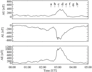
Fig. 1. The AE, AL and AU -indices of 31 July 1997. The letters
a–h correspond to the time periods when we have measurements from PIXIE and UVI.
X-ray distribution over the entire polar region at the same time. It took about 17 min for the DMSP X-ray spectrometer to make a complete image. They also had to use interpola-tion routines to fill spatial data gaps in the coverage of the instrument.
The X-ray camera PIXIE and the UV imager UVI onboard the Polar satellite provide global information about the elec-tron precipitation and how it varies both in time and space. We can derive the precipitating electron spectrum by analyz-ing the UV-emissions and the X-rays. The UVI camera is most sensitive to the softer electron energies. Electron spec-tra derived from UV emissions will include all electrons re-sponsible for the Pedersen conductance, while the estimation of a proper Hall conductance is more uncertain. A similar but opposite scheme is valid for the PIXIE camera. Electron spectra derived from X-ray measurements provide good cov-erage of the higher electron energies contributing to the Hall conductance. The estimation of a proper Pedersen conduc-tance is more problematic as PIXIE cannot measure X-rays produced by electrons lower than a few keV. By combin-ing both PIXIE and UVI measurements we can, however, cover the whole electron energy range between about 0.1 and 100 keV, as pointed out by Østgaard et al. (2001). We are therefore able to capture also the high-energy tail of the auroral electron spectrum.
In this paper, we make use of X-ray and UV-emission mea-surements of an isolated substorm event, occurring, approx-imately, between 02:45 and 04:00 UT on 31 July 1997, to derive instantaneous global conductance maps. The AE-index, which we present in Fig. 1, gives indications of a rather intense substorm as the values exceed 1000 nT around 03:00 UT. This substorm occurred in the beginning of a small magnetic storm, although the Dst index only decreased from
14 to −20 nT during a 3 h period. The letters a–h correspond to the time periods when we have measurements from PIXIE and UVI.
2 The procedure: From X-ray and UV-emissions to con-ductance values
2.1 From X-ray measurements to electron spectra
PIXIE is a pinhole camera detecting X-ray photons (Imhof et al., 1995). The useful energy range of these photons is approximately between 2 and 22 keV.
A technique for deriving a four-parameter electron spectral distribution from the measured X-ray spectra is described in Østgaard et al. (2000). We only present a brief description here.
To establish the electron spectra causing the measured X-rays, we make use of a look-up table provided by a cou-pled electron photon transport code originally derived from neutron transport codes (Lorence, 1992). This look-up table gives us the X-ray production emitted at different zenith an-gles for electrons with different exponential energy spectra. Isotropic electron precipitation has been assumed.
As described by Østgaard et al. (2001), the X-ray mea-surements are divided into 120 boxes. A box is 6 corrected geomagnetic (CGM) degrees latitude by 1 h MLT, starting at CGM latitude 52◦ until 82◦. From the X-ray spectrum measured in each box, we derive a corresponding electron spectrum by using the look-up table as described above. 2.2 From UV emission measurements to electron spectra We will give a short description of the method used to derive the average electron energy and the electron energy flux from UV-emissions measured by the UVI camera. For a more de-tailed description, see Germany et al. (1997, 1998a, b).
Global images of emissions within the Lyman-Birge-Hopfield (LBH) band (140–180 nm) are provided by the UVI instrument (Torr et al., 1995). The LBH-emissions are divided into LBHS (140–160 nm) and LBHL (160– 180 nm) respectively. Within the UVI band pass, the O2
Schumann-Runge absorption continuum peaks at the shorter wavelengths and decreases with longer wavelengths. Thus, the shorter wavelengths (LBHS) are subject to significantly greater O2absorption than the longer wavelengths (LBHL).
The height level for production of UV emissions depends on the incoming electron energy. Electrons of higher ener-gies deposit their energy deeper in the atmosphere, resulting in a stronger absorption of the UV-emissions as they propa-gate out of the atmosphere.
The average electron energy is derived from the ratio of the intensities of the two LBH bands using an assumed spectral shape. Similarly, the energy flux is derived from the LBHL intensity.
2.3 Electron spectra derived from both PIXIE and UVI measurements
We use the average electron energy and the electron energy flux from UVI measurements to fit an exponential as well as a Maxwellian distribution. The final choice of spectrum for the lower electron energy range depends on which one gives
Table 1. Maximum Hall and Pedersen conductance in magnitude and location for the isolated substorm event on 31 July 1997, as derived
from the combined PIXIE and UVI measurements as well as from UVI data only. We also present the differences in percent between the conductance values using electron spectra derived from both PIXIE and UVI compared with the values obtained using spectra derived from UVI only. The letters a–h correspond to the 8 time periods as given in Fig. 2
Hall conductance Pedersen conductance Time MLT UVI PIXIE Difference: UVI PIXIE Difference:
Period Sector [S] +UVI UVI vs + UVI UVI vs
[S] PIXIE + UVI [S] [S] PIXIE + UVI
[%] [%] (a)* 20:00–21:00 28 27 −3.6 15 15 0.0 (b) 23:00–00:00 47 53 13 25 25 0.0 (c) 01:00–02:00 41 51 24 22 22 0.0 (d) 03:00–04:00 24 29 21 12 12 0.0 (e) 01:00–02:00 17 23 35 7.6 7.8 2.6 05:00–06:00 19 23 21 8.7 8.9 2.3 (f) 08:00–09:00 16 21 31 7.8 8.0 2.6 (g) 08:00–09:00 18 20 11 7.7 7.7 0.0 09:00–10:00 15 20 33 6.6 6.8 3.0 (h) 06:00–07:00 12 16 33 5.3 5.5 3.8 08:00–09:00 12 16 33 5.8 6.0 3.4
* Note that in our method the upper energy limit of the UVI spectrum is lower when merged with the PIXIE spectrum than is its value when UVI is used alone. As a result, under some circumstances, for example, during the time period 02:30:40–02:35:10 UT (row (a)), larger conductances can be obtained from the UVI only spectrum than from the UVI plus PIXIE spectrum.
the smoothest transition to the exponential electron spectrum derived from the measured X-ray spectrum.
For this particular event, 31 July 1997, Østgaard et al. (2001) have compared measured electron spectra, from the polar orbiting satellites DMSP F14 and NOAA 12, with de-rived electron spectra from the PIXIE and UVI measure-ments. Regarding the energy flux between 90 eV and 30 keV, they find an average ratio of 1.03 ± 0.6 by comparing mea-sured and derived electron spectra, indicating good agree-ment. The polar orbiting satellites measure the electron fluxes, only along a line through the large pixels of about 700 km × 700 km in the PIXIE measurements. Thus the electron fluxes measured by these satellites are not necessar-ily the same as the average electron flux in the corresponding PIXIE pixel. This explains the large standard deviation. 2.4 Deriving the conductance values from the energy
spec-tra
We use a computer code developed by University of Mary-land based on the TANGLE code (for more details on TAN-GLE, see Vondrak and Baron, 1976; Vondrak and Robinson, 1985). The code models the ionospheric effects of energy de-position into the atmosphere by energetic particles. One pos-sible output is conductivity. Input is the electron spectrum as derived from PIXIE and UVI measurements. To model the atmosphere, the program code uses the Mass Spectrometer and Incoherent Scatter Extended Atmospheric model (MSIS-E-90). The electron energy deposition function is the cosine-dependent Isotropic over the Downward Hemisphere (IDH)
model of Rees (1963). Rees (1989) has also contributed an expression for the electron range function.
First, the electron production q from the precipitation is calculated. We should point out that q does not include any contribution from the solar illumination. The dayglow has been removed from the UVI images and the background originating from other sources than particle precipitation has been removed from the PIXIE data. To establish a value of the total electron density Ne, we therefore have to include
a background electron source term q0in the time-dependent
rate equation:
dNe/dt = q(h) + q0(h) − αeff(h) ∗ Ne2(h) (1)
q0 is taken from the International Reference Ionosphere
(IRI)-95 model, which is an empirical standard model of the ionosphere. αeff is the effective dissociative recombination
coefficient. The program uses formulas derived from Vick-rey et al. (1982) and Gledhill (1986) to calculate αeff. We
should point out that we have not included diffusive transport in the equation as this is negligible at the heights contribut-ing to the conductances. Chemical equilibrium is assumed, since the recombination time is on the order of seconds. We therefore set dNe/dt =0.
Finally the code derives the conductivities, using ion-neutral collision frequencies from Vickrey et al. (1981) and electron-neutral collision frequencies from Thrane and Pig-gott (1966).
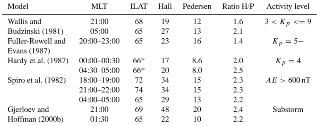
Table 2. Maximum Hall and Pedersen conductance in magnitude and location for five statistical conductance models
Model MLT ILAT Hall Pedersen Ratio H/P Activity level
Wallis and 21:00 68 19 12 1.6 3 < Kp<=9 Budzinski (1981) 05:00 65 27 13 2.1 Fuller-Rowell and 20:00–23:00 65 23 16 1.4 Kp=5− Evans (1987) Hardy et al. (1987) 00:00–00:30 66* 17 8.6 2.0 Kp=4 04:30–05:00 66* 20 8.0 2.5 Spiro et al. (1982) 18:00–19:00 72 34 15 2.3 AE >600 nT 21:00–22:00 74 34 15 2.3 04:00–05:00 65 29 13 2.2
Gjerloev and 21:00 69 48 20 2.4 Substorm
Hoffman (2000b) 01:30 65 22 10 2.2
* Note that the model of Hardy et al. (1987) uses CGM latitudes. The other models give the position in invariant latitude (ILAT).
3 Results
In Fig. 2, we present global maps of how the conductances derived from combined PIXIE and UVI measurements vary during this isolated substorm. A new X-ray image is pro-duced from the PIXIE measurements every 15 min with an integration time of about 4.5 min. UVI images were selected to match the PIXIE observations. This procedure has been explained by Østgaard et al. (2001) in detail. Østgaard et al. (2000) have analyzed the electron precipitation during this event, and they have shown that substorm onset occurs at 02:40:30 UT in the MLT sector 20:00–21:00. We have derived the global distribution of conductance and we have images showing the conductances before substorm onset (Fig. 2a), during the substorm expansion and recovery phase (Fig. 2b–g) and until the end of recovery phase (Fig. 2h). Also presented in Fig. 2 are global maps of Hall to Pedersen conductance ratios. We require the Pedersen conductance to be greater than 4 s in order to calculate a Hall to Pedersen conductance ratio.
Our results give the strongest conductances in the sub-storm onset region in the pre-midnight sector (Fig. 2b). Here we find a maximum Hall conductance value of 53 s and a maximum Pedersen conductance of 25 s, as presented in Table 1.
By looking at the successive conductance maps in Fig. 2, we find that the Hall conductance maximum remains situated between CGM latitudes 64–70◦ during the whole substorm event. The image before substorm onset (Fig. 2a) places the Hall conductance maximum in the MLT sector 20:00–21:00. This maximum moves eastward with every subsequent data set, as presented in Table 1.
The scatter in Fig. 2 may reflect the uncertainty in deriving proper electron energy spectra. Boxes marked with a black dot indicate that we have only included the background elec-tron density when deriving the conductances although there may be some weak precipitation.
We have calculated the conductance values using electron
spectra derived from both PIXIE and UVI; we compared these with the values obtained using spectra derived from UVI only. This is done in order to examine how sensitive the conductance values are to the energetic tail in the energy spectra. The study is motivated by the fact that most of the statistical conductance models presented are based on mea-surements of precipitating electrons at energies below ap-proximately 30 keV. Since the UVI LBHS intensity decreases significantly at higher electron energies, the UVI electron en-ergy range is more or less comparable with the enen-ergy ranges of most of the statistical models. Therefore, in Table 1, we have also included conductance values derived from UVI measurements only. We find that combining PIXIE and UVI results in significantly greater Hall conductance values. This is due to the fact that PIXIE captures the high energy tail of the precipitating electron energy spectra while UVI mea-surements do not provide sufficient information to derive the spectral shape of these high electron energies. We find only minor differences for the Pedersen conductance. This was to be expected, as UVI measures well the softer electron ener-gies which are most significant to the Pedersen conductance. The differences between conductance values deduced from both PIXIE and UVI measurements and conductance values from using UVI only have been studied more closely. In Fig. 3, we present such differences for six MLT sectors. Note that we are looking at data from CGM latitudes 64–70◦, since
this is the area of maximum conductance (see Fig. 2). We have further disregarded data when the Hall conductances, estimated from the UVI measurements, are lower than 7 s, in order to avoid using uncertain conductance values. The mean difference in the Hall conductance estimated for MLT sectors 18:00–21:00 is ∼36%. This means that the Hall con-ductances derived when combining PIXIE and UVI are about 36% greater than the values derived from UVI data only. In the next MLT sector, between 21:00–24:00, we find a some-what lower mean difference of about 21% in the Hall con-ductances. Thereafter, this mean value exceeds ∼24, ∼26 and ∼29%, respectively, for the MLT sectors 00:00–03:00,
Time [UT]
a
0230:40
-0235:10
b
0245:40
-0250:10
c
0300:30
-0305:00
d
0315:40
-0320:10
ΣH [S] ΣP [S] ΣH/ΣPFig. 2. Polar plots of the Hall and Pedersen conductances for 8 successive time periods during the isolated substorm event on 31 July 1997.
Boxes where we have only included the contribution to the conductances from the background are marked with a black dot. Also presented are the Hall to Pedersen conductance ratios.
03:00–06:00 and 06:00–09:00. A mean difference in the Hall conductance value of ∼ 48% for the last MLT sector between 09:00 and 12:00 indicates a hardening of the electron spectra on the morningside.
4 Discussion
A comparison between our instantaneous global conductance maps and the statistical models has been done. In order to do
such a comparison, we make use of the AE and Kpindices.
Except for the model by Gjerloev and Hoffman (2000b), all the statistical models presented depend strongly on either the value of the AE index or the Kp index. Usually, the AE
in-dex should be the best correlation parameter. While Kp is a
3 h index, AE can be estimated every minute. However, for this event on 31 July 1997, only four geomagnetic stations have contributed to the provisional AE index. This implies a probability that electrons may precipitate in a region not
Time [UT]
e
0330:40
-0335:10
f
0345:40
-0350:10
g
0400:40
-0403:50
h
0415:40
-0420:00
ΣH [S] ΣP [S] ΣH/ΣP Fig. 2. continued ...covered by the stations contributing to this AE index. From Fig. 2, we find that the strongest conductances are present in the time period 02:45:40–02:50:10 UT. According to Fig. 1, this takes place while the AE index is still rather low al-though, by looking at magnetic field data from the Cana-dian magnetometer station at Fort Churchill located in the region of the precipitation, we observe abrupt decreases in the magnetic field measurements around 02:45 UT. Conse-quently, we must be cautious when comparing the AE index and the global conductance distribution for this case.
Since we have instantaneous data, we have a tool to study
the time development of the conductivities. However, the spatial resolution of the PIXIE camera is a severe restriction, as it is ∼700 km. This prevents us from studying small scale features and gradients.
As presented in Table 2, most of the statistical models have several conductance maximum regions. Our instantaneous global conductance maps (Fig. 2) show only one maximum for most of the time periods presented.
In Table 2, we have summarized published Hall to Ped-ersen conductance ratios. We find that this parameter varies between 1.4 and 2.5.
Fig. 3. Differences between conductances derived from the
com-bined PIXIE and UVI measurements and conductances derived from UVI data only. We study six different MLT sectors for CGM latitudes 64–70◦. The differences are given in percent. The letters a–h correspond to the 8 time periods given in Fig. 2.
The Hall to Pedersen conductance ratios derived from our measurements are given in Table 3. Ratios are given for con-ductances derived from combined PIXIE and UVI as well as from UVI only. We study the same regions as those given in Table 1 but now we have not included the contribution of the background density. This is done because all the conduc-tance models (except Wallis and Budzinski, 1981) only take precipitation data into account. It is interesting to note that the ratios derived from using UVI measurements only are in the same range as the ratio values from the different conduc-tance models (Table 2). The ratios derived from combining PIXIE and UVI are on the average ∼20% greater. Since the statistical models in Table 2 operate with almost the same electron energy detection range as the UVI imager, we sug-gest, therefore, that the statistical models presented probably underestimate the Hall conductance. Consequently, the Hall to Pedersen conductance ratio depends strongly on whether or not we include the PIXIE measurements. This ratio is of-ten used as an indicator of the hardness of the precipitating electrons. For example, Brekke et al. (1989) derived an em-pirical formula between the root-mean-square energy of the precipitating electrons and the Hall to Pedersen conductance ratio. Germany et al. (1994), using a different approach, found a power law dependence of conductances on the en-ergy flux.
A different kind of underestimation was pointed out by Robinson et al. (1987). They came up with empirical formu-lae relating Hall and Pedersen conductances to the average
Table 3. The Hall to Pedersen conductance ratios derived from the
combined PIXIE and UVI measurements, as well as from UVI data only, for the regions of maximum conductance (given in Table 1). The letters a–h correspond to the 8 time periods given in Fig. 2. Background electron density is not included
Time MLT UVI PIXIE & UVI
Radio H/P Radio H/P (a) 20:00–21:00 1.9 1.8 (b) 23:00–00:00 1.9 2.1 (c) 01:00–02:00 1.9 2.3 (d) 03:00–04:00 2.1 2.4 (e) 01:00–02:00 2.3 2.9 05:00–06:00 2.2 2.6 (f) 08:00–09:00 2.1 2.7 (g) 08:00–09:00 2.4 2.7 09:00–10:00 2.4 3.1 (h) 06:00–07:00 2.4 3.0 08:00–09:00 2.2. 2.9
energy and energy flux of the electrons. According to Robin-son et al. (1987), it is essential to integrate over a broad elec-tron energy range when calculating the mean energy value. However, errors do arise in the application of their equations if too many lower electron energies are included. They sug-gest a lower limit of 500 eV as secondary electron fluxes be-come important at energies below. As Spiro et al. (1982) estimated a mean energy value and thereafter the conduc-tivities from an electron detection range of 0.2–27 keV, they probably underestimated the conductances in two ways. First of all, they included too many lower electron energies in the calculation of the total number flux. These lower electron energies deposit their energy too high in the atmosphere to affect conductances and should therefore not be included in the calculation of a mean energy value. When the energy flux is divided by the number flux including these low energies, the resulting values of mean energy cannot be used in the empirical relations for conductance. Secondly, they should have extrapolated their spectra to higher energies, according to Robinson et al. (1987). Hardy et al. (1987) took the results of Robinson et al. (1987) into account, as they both intro-duced a low-energy cutoff of approximately 500 eV as well as an extrapolation of the spectra to 100 keV before estimat-ing the mean energy value. However, Hardy et al. (1987) will not capture the high energy tail, as pointed out in the introduction.
We find that a combination of both PIXIE and UVI mea-surements is needed in order to cover all electron energies contributing to the conductances. However, our results also underestimate the conductances since the proton precipita-tion will not contribute to the X-ray measurements. The UVI camera is thought to be partly sensitive to protons also. Ac-cording to Frey et al. (2001), LBH emission may contain con-tributions from proton excitation, although this is limited to localized regions with great proton precipitation. The model
by Fuller-Rowell and Evans (1987) is the only model pre-sented, based on particle detection, which takes into account this contribution. Fuller-Rowell and Evans have included the proton energy flux in their calculation by treating the protons as if they were electrons. According to Galand et al. (2001), electrons are the dominant source of ionization. In a sta-tistical study during moderate magnetic activity (Kp = 3),
they found that protons contributed ∼15% to the total en-ergy inferred although this is strongly dependent upon loca-tion. This result is similar to an earlier study by Hardy et al. (1989), which found that the hemispheric energy input from the ions varied between 11 and 17% of the energy input for the electrons.
From Table 3, we observe that the Hall to Pedersen con-ductance ratio for regions of maximum Hall concon-ductance is increasing throughout the event. This indicates a hardening of the electron spectra as the maximum moves to the morn-ingside.
Around substorm onset, at 02:45:40–02:50:10 UT, we find, from Fig. 2, several boxes in the pre-midnight sec-tor showing a strong Hall conductance. From 20:00 to 00:00 MLT, the Hall conductance is between 48 and 53 s. The maximum Hall conductance values in the pre-midnight sector from the previous studies varies between 19 s (Wallis and Budzinski, 1981), 23 s (Fuller-Rowell and Evans, 1987) and 34 s (Spiro et al., 1982). A qualitative comparison be-tween such maximum values is difficult. First of all, sub-storms are highly variable and we compare results from just one substorm event with models based on average values. We should point out that our conductance maximum value is associated with the start of the substorm expansion phase, when energy is loaded into the ionosphere. We also have a significant difference in spatial resolution. Most of the statistical conductance models bin their values in a 1◦ lati-tude grid. When using PIXIE and UVI measurements, we have to include data from six degrees latitude (as pointed out in Sect. 2.1) in order to derive reliable electron spectra and thereafter conductance values. The time resolution is also in favor of the statistical models as the integration time is mea-sured in seconds while PIXIE and UVI estimates require sev-eral minutes of data. This leaves us with lower values than a better resolution in both space and time would give us. How-ever, while we have the possibility to present instantaneous values, the statistical models must take into account a great number of measurements. This will result in a smoothing of the conductance values and thereby a reduction compared to the peak values of individual measurements. Finally, as al-ready pointed out, the statistical models probably underesti-mate the Hall conductance whenever a hard electron spectral component is present.
The statistical model of Gjerloev and Hoffman (2000b) reports a Hall conductance value of 48 s. This is a signifi-cantly greater value than the maxima from the other statisti-cal conductance models. By organizing their data according to the electrodynamical signature of the substorm instead of using MLT, they avoid a mixing of data from different parts of the substorm. Further, they have restricted their model of
conductances to time periods with auroral substorms. The main reason for the high conductance values of Gjerloev and Hoffman (2000a) is the fine spatial resolution in the mea-surements of the precipitation events, allowing them to iden-tify Hall conductance peaks exceeding 100 s. Such values are reported to have a typical size of ∼20 km and are asso-ciated with energetic (>10 keV) inverted V events. With our much coarser spatial resolution (∼700 km), we are not able to identify such small scale features by using PIXIE and UVI measurements.
Kirkwood et al. (1988) used the European Incoherent Scat-ter (EISCAT) radar to examine the conductivity changes dur-ing substorms. They selected seven substorm events and measured the electron density profile in order to calculate the conductances. By using the incoherent scatter radar, they could produce electron density profiles with high resolution in both altitude (2 km) and time (5 s). In accordance with Gjerloev and Hoffman (2000b), Kirkwood et al. found Hall conductance values exceeding 100 s, the highest Hall and Pedersen conductances reaching 120 s and 48 s, respectively; they could not, however, present the global conductance dis-tribution as radar measurements are localized to small re-gions.
We observe that the conductance maximum moves east-ward throughout the substorm event. In the later phases of the substorm, the conductance maximum is found on the morningside. This can be associated with the maximum in the energetic electron precipitation which typically develops in the dawn region during substorms (Østgaard et al., 2000). A maximum on the morningside is also seen in several previ-ous studies (Wallis and Budzinski, 1981; Spiro et al., 1982; Hardy et al., 1987).
From Fig. 2, we find that the location of the maximum Hall conductance for all time periods is between CGM lati-tudes 64–70◦. This corresponds well with the different model results, as presented in Table 2.
5 Conclusion
By using X-ray data from PIXIE and UV emission data from UVI, we can derive the energy spectrum and the fluxes of the precipitating energetic electrons over a wide energy range. We can then calculate the associated ionization and conduc-tances in the upper atmosphere.
In this paper, we have shown that a combination of PIXIE and UVI data is needed in order to cover the whole electron energy range influencing the conductivities. By deriving con-ductivities from UVI data only, we find that the Hall conduc-tance is underestimated. This underestimation is strongest in MLT sector 09:00–12:00 for the isolated substorm event of 31 July 1997. Including PIXIE measurements gives Hall conductance values approximately 48% greater than those deduced from UVI only. Most of the existing statistical mod-els have derived the conductivities by detecting electrons in an energy range comparable with the UVI imager. We there-fore suggest that these statistical models underestimate the
Hall conductance. This is further supported by an analysis of the Hall to Pedersen conductance ratio. From UVI mea-surements only, we derive values comparable with the model results. However, introducing PIXIE data results in signifi-cantly greater Hall to Pedersen conductance ratio values.
In contrast to statistical conductance models, we can study the time development of the conductances throughout a spe-cific substorm event by using PIXIE and UVI measurements. For the isolated substorm event occurring on 31 July 1997, we have generated global maps of the Hall and Pedersen con-ductances. The strongest conductances are observed in the substorm onset region in the pre-midnight sector. The Hall conductance maximum remains situated between CGM lat-itudes 64–70◦ during the whole substorm event and moves eastward. In the late recovery phase of the substorm, we ob-serve a conductance maximum in the dawn region. The Hall to Pedersen conductance ratio for the locations with maxi-mum Hall conductance is increasing throughout the event. This indicates a hardening of the electron spectra as the con-ductance maximum moves eastward on the morningside.
Acknowledgements. This study was supported by the Norwegian Research Council (NFR).
The work was also supported by NASA UVI funding from Univer-sity of California, Berkeley grant SA3216 to the UniverUniver-sity of Al-abama in Huntsville, by contract F49620-00-0-0204 from the Air Force Office of Scientific Research and by NASA grant NAG5-10743 (G. A. Germany).
Work at the University of Maryland has been supported by NASA contract NAS5-30372 under Subcontract No. SE70A0470R from the Lockheed Martin Advanced Technology Center.
J. Stadsnes thanks the staff of the NASA/GSFC Laboratory for Ex-traterrestrial Physics for their hospitality and support during his stay in 2000.
We are grateful to COSPAR and URSI for generating and making available via the Internet, IRI-95 an empirical standard model of the ionosphere.
We are also grateful to the World Data Center – C2 (T. Kamei) in Kyoto, Japan, for making quick look AE indices available via the Internet.
Topical Editor M. Lester thanks R. M. Robinson and another ref-eree for their help in evaluating this paper.
References
Ahn, B.-H., Robinson, R. M., Kamide, Y., and Akasofu, S.-I.: Elec-tric conductivities, elecElec-tric fields and auroral particle energy in-jection rate in the auroral ionosphere and their empirical relations to the horizontal magnetic disturbances, Planet. Space. Sci., 31, 641, 1983.
Ahn, B.-H., Kroehl, H. W., Kamide, Y., and Gorney, D. J.: Estima-tion of ionospheric electrodynamic parameters using ionospheric conductance deduced from bremsstrahlung X ray image data, J. Geophys. Res., 94, 2565, 1989.
Ahn, B.-H., Richmond, A. D., Kamide, Y., Kroehl, H. W., Emery, B. A., de la Beaujardiere, O., and Akasofu, S. I.: An ionospheric conductance model based on ground magnetic disturbance data, J. Geophys. Res., 103, 14 769, 1998.
Brekke, A., Hall, C., and Hansen, T. L.: Auroral ionospheric con-ductances during disturbed conditions, Ann. Geophysicae, 7, 269, 1989.
Chapman, S.: The electrical conductivity of the ionosphere: A re-view, Nuovo Cimento, 4, 1385, 1956.
Frey, H. U., Mende, S. B., Carlson, C. W., Gerard, J.-C., Hubert, B., Spann, J., Gladstone, R., and Immel, T. J.: The electron and proton aurora as seen by IMAGE-FUV and FAST, Geophys. Res. Lett., 28, 1135, 2001.
Fujii, R., Hoffman, R. A., Anderson, P. C., Craven, J. D., Sugiura, M., Frank, L. A., and Maynard, N. C.: Electrodynamical parame-ters in the nighttime sector during auroral substorms, J. Geophys. Res., 99, 6093, 1994.
Fuller-Rowell, T. J. and Evans, D. S.: Height-integrated Pedersen and Hall conductivity patterns inferred from the TIROS-NOAA satellite data, J. Geophys. Res., 92, 7606, 1987.
Galand, M., Fuller-Rowell, T. J., and Codrescu, M. V.: Response of the upper atmosphere to auroral protons, J. Geophys. Res., 106, 127, 2001.
Germany, G. A., Torr, D. G., Richards, P. G., Torr, M. R., and John, S.: Determination of ionospheric conductivities from FUV auro-ral emissions , J. Geophys. Res., 99, 23 297, 1994.
Germany, G. A., Parks, G. K., Brittnacher, M., Cumnock, J., Lum-merzheim, D., Spann, J. F., Chen, L., Richards, P. G., and Rich, F. J.: Remote determination of auroral energy characteristics dur-ing substorm activity, Geophys. Res. Lett., 24, 995, 1997. Germany, G. A., Parks, G. K., Brittnacher, M., Spann, J. F.,
Cum-nock, J., Lummerzheim, D., Rich, F. J., and Richards, P. G.: En-ergy characterization of a dynamic auroral event using GGS UVI images, in Geospace Mass and Energy Flow: Results from the In-ternational Solar-Terrestrial Physics Program, edited by Horwitz, J. L., Gallagher, D. L., and Peterson, W. K., AGU, Washington, D.C., 143, 1998a.
Germany, G. A., Spann, J. F., Parks, G. K., Brittnacher, M., Elsen, R., Chen, L., Lummerzheim, D., and Rees, M.: Auroral obser-vations from the Polar Ultraviolet Imager (UVI), in Geospace Mass and Energy Flow: Results from the International Solar-Terrestrial Physics Program, edited by Horwitz, J. L., Gallagher, D. L., and Peterson, W. K., AGU, Washington, D.C., 149, 1998b. Gjerloev, J. W. and Hoffman, R. A.: Height-integrated conductivity in auroral substorms. 1. Data, J. Geophys. Res., 105, 215, 2000a. Gjerloev, J. W. and Hoffman, R. A.: Height-integrated conductivity in auroral substorms. 2. Modelling, J. Geophys. Res., 105, 227, 2000b.
Gledhill, J. A.: The effective recombination coefficient of electrons in the ionosphere between 50 and 150 km, Radio Sci., 21, 3, 339, 1986.
Goldberg, R. A., Barcus, J. R., Treinish, L. A., and Vondrak, R. R.: Mapping of auroral X rays from rocket overflights, J. Geophys. Res., 87, 2509, 1982.
Hardy, D. A., Gussenhoven, M. S., Vaistrick, R., and McNeil, W. J.: Statistical and functional representations of the pattern of auroral energy flux, number flux, and conductivity, J. Geophys. Res., 92, 12, 275, 1987.
Hardy, D. A., Gussenhoven, M. S., and Brautigam, D.: A Statistical Model of Auroral Ion Precipitation, J. Geophys. Res., 94, 370, 1989.
Imhof, W. L., Spear, K. .A., Hamilton, J. W., Higgins, B. R., Mur-phy, M. J., Pronko, J. G., Vondrak, R. R., McKenzie, D. L., Rice, C. J., Gorney, D. J., Roux, D. A., Williams, R. L., Stein, J. A., Bjordal, J., Stadsnes, J., Njoten, K., Rosenberg, T. J., Lutz, L., and Detrick, D. L.: The Polar Ionospheric X-ray Imaging
Exper-iment (PIXIE), Space Sci. Rev., 71, 385, 1995.
Kirkwood, S., Opgenoorth, H., and Murphree, J. S.: Ionospheric conductivities, electric fields and currents associated with auroral substorms measured by the EISCAT radar Planet. Space. Sci., 36, 1359, 1988.
Lorence, L. J.: CEPXS/ONELD Version 2.0: A discrete ordinates code package for general one-dimensional coupled electron-photon transport, IEES Trans. Nucl. Sci, 39, 1031, 1992. Lummerzheim, D., Rees, M. H., Craven, J. D., and Frank, L. A.:
Ionospheric conductances derived from DE-1 auroral images, J. atmos. terr. Phys., 53, 281, 1991.
Meng, C.-I., Mauk, B., and McIlwain, C. E.: Electron precipitation of evening diffuse aurora and its conjugate electron fluxes near the magnetospheric equator, J. Geophys. Res., 84, 2545, 1979. Miller, K. L. and Vondrak, R. R.: A high-latitude phenomenological
model of auroral precipitation and ionospheric effects Radio Sci., 20, 3, 431, 1985.
Østgaard, N., Stadsnes, J., Bjordal, J., Vondrak, R. R., Cummer, S. A., Chenette, D., Schulz, M., and Pronko, J.: Cause of the localized maximum of X-ray emission in the morning sector: A comparison with electron measurements, J. Geophys. Res., 105, 20 869, 2000.
Østgaard, N., Stadsnes, J., Bjordal, J., Germany, G. A., Vondrak, R. R., Parks, G. K., Cummer, S. A., Chenette,D., and Pronko, J.: Auroral electron distributions derived from combined UV and X-ray emissions, J. Geophys. Res., 106, 26 081, 2001.
Rees, M. H.: Auroral ionization and excitation by incident energetic electrons, Planet. Space. Sci., 11, 1209, 1963.
Rees, M. H., Lummerzheim, D., Roble, R. G., Winningham, J. D., Craven, J. D., and Frank, L. A.: Auroral energy deposition rate, characteristic electron energy, and ionospheric parameters
de-rived from Dynamics Explorer 1 images, J. Geophys. Res., 93, 12, 841, 1988.
Rees, M. H.: Physics and Chemistry of the Upper Atmosphere, Cambridge Univ. Press, Cambridge, UK, 1989.
Robinson, R. M., Vondrak, R. R., Miller, K., Dabbs, T., and Hardy, D.: On calculating ionospheric conductances from the flux and energy of precipitating electrons, J. Geophys. Res., 92, 2565, 1987.
Spiro, R. W., Reiff, P. H., and Maher Jr., L. J.: Precipitating electron energy flux and auroral zone conductances – an empirical model, J. Geophys. Res., 87, 8215, 1982.
Thrane, E. V. and Piggott, W. R.: The collision frequency in the E- and D-regions of the ionosphere, J. Atmos. Terres. Phys., 28, 721, 1966.
Torr, M. R., Torr, D. G., Zukic, M., Johnson, R. B., Ajello, J., Banks, P., Clark, K., Cole, K., Keffer, C., Parks, G., Tsurutani, B., and Spann, J.: A far ultaviolet imager for the international solar-terrestrial physics mission, Space Sci. Rev., 71, 329, 1995. Vickrey, J. F., Vondrak, R. R., and Matthews, S. J.: Energy depos-tion by energetic particles and Joule dissipadepos-tion in the auroral ionosphere, J. Geophys. Res., 86, 65, 1981.
Vickrey, J. F., Vondrak, R. R., and Matthews, S. J.: The diurnal and latitudinal variation of auroral zone ionospheric conductivity, J. Geophys. Res., 87, 5148, 1982.
Vondrak, R. and Robinson, R.: Inference of high-latitude ionization and conductivity from AE-C measurements of auroral electron fluxes, J. Geophys. Res., 90, 7505, 1985.
Vondrak, R. R. and Baron, M. J.: Radar measurements of the lat-itudinal variation of auroral ionization, Radio Sci., 11, 11, 939, 1976.
Wallis, D. D. and Budzinski, E. E.: Empirical models of height integrated conductivities, J. Geophys. Res., 86, 125, 1981.