Ionospheric composition measurement by EISCAT using a global fit procedure

HAL Id: hal-00329062

https://hal.archives-ouvertes.fr/hal-00329062

Submitted on 1 Jan 1996

HAL is a multi-disciplinary open access

archive for the deposit and dissemination of sci-entific research documents, whether they are pub-lished or not. The documents may come from teaching and research institutions in France or abroad, or from public or private research centers.

L’archive ouverte pluridisciplinaire HAL, est destinée au dépôt et à la diffusion de documents scientifiques de niveau recherche, publiés ou non, émanant des établissements d’enseignement et de recherche français ou étrangers, des laboratoires publics ou privés.

Ionospheric composition measurement by EISCAT using

a global fit procedure

B. Cabrit, W. Kofman

To cite this version:

B. Cabrit, W. Kofman. Ionospheric composition measurement by EISCAT using a global fit procedure. Annales Geophysicae, European Geosciences Union, 1996, 14 (12), pp.1496-1505. �hal-00329062�

Correspondence to: B. Cabrit

Ann. Geophysicae 14, 1496—1505 (1996) ( EGS — Springer-Verlag 1996

Ionospheric composition measurement by EISCAT using

a global fit procedure

B. Cabrit, W. Kofman

CEPHAG ENSIEG, URA 346 CNRS, Grenoble, France

Received: 4 March 1996/Revised: 17 June 1996/Accepted: 3 July 1996

Abstract. The aim of this paper is to show the gain of the global fit procedure compared to the classical gate-by-gate analysis in the simultaneous determination of the temperatures and composition profiles in the lower F region. A method for the evaluation of the transition altitude and the width of the transition region between molecular and atomic ions is described in the case of the EISCAT CP1 experiment; it is validated using a simulated experiment. It is shown that alternating-code gates have to be processed together with the long-pulse gates. Our new method is applied on six days of actual data. The results obtained during quiet periods are compared with independent estimations.

1 Introduction

For more than 20 years, incoherent scatter has proved to be a very powerful technique for ionospheric probing. Extensive studies (Salpeter, 1960; Dougherty and Farley, 1960; Hagfors, 1961; Evans, 1969) have shown the rela-tionship between radar spectra and ionospheric para-meters. Based on these earlier results, incoherent-scatter facilities like EISCAT were built in order regularly to monitor the ionospheric activity.

In practice, it is impossible to measure simultaneously all the parameters on which the radar signal depends, i.e. the density, the velocity and the temperature of each charged species. Depending on the altitude region, it is necessary to introduce suitable assumptions in order to close the inversion problem. The ‘‘classical’’ approach used to monitor the ionosphere by EISCAT consists in the extraction of four parameters from incoherent spectra: electron density, electron temperature, ion temperature and bulk velocity. Other parameters are either given by

additional constraints or by empirical models. This is the case of the relative abundance of molecular ions which is taken from a time-independent empirical profile. Indeed the simultaneous determination of the temperatures and the composition fails most of the time due to the correla-tion between these parameters in the spectral form deter-mination. Many strategies have been proposed to address the composition.

In Oliver (1979) the ion temperature in the transition region was modelled with a Bates profile. With this given temperature, the fit of the composition in the transition region became possible. This method is limited to non-disturbed periods, when the contribution of the frictional ion heating to the temperature profiles is negligible. An application to auroral scatter data is then difficult, and Kelly and Wickwar (1981) proposed an alternative method for handling Joule-heating events. In this case the electron temperature is constrained with its measurements made before and after the ions are heated. In this method the electron-temperature profile is supposed to remain constant during the event.

Lathuille`re et al. (1983b) did perform a simultaneous fit of the temperature and composition. This method is lim-ited to data with good SNR (signal-over-noise ratio), coming from large scattering volumes. The results need to be smoothed over few hours. It was used to address the daily and seasonal variation of the composition profile. Nevertheless, inferred parameters from large scattering volume suffer a bias which is very difficult to evaluate a posteriori. An independent determination of temper-atures and composition from incoherent-scatter data is still a challenge.

In the last few years new techniques have been de-veloped in order to correct the range smearing effect. The inversion program OASIS, developed and tested for Millestone Hill scatter radar (Holt et al., 1992) uses cubic splines as the line-of-sight plasma parameter profile model, and performs a global regression on the spline coefficients. In these previous studies, the inver-sion method, also called ‘‘full-profile’’, was analysed in terms of gain in the range resolution. It was limited

to classical parameter fitting (see also Lethinen, this issue).

We propose to use the global-regression technique for the simultaneous determination of the temperature and composition of the ionosphere from CP1-experimental data. A similar approach can be used for solving the problem of the simultaneous determination of the colli-sion frequency and the temperatures at low altitude, be-low 110 km (see Lathuille`re et al., 1983a; Kofman and Lathuille`re, 1985). The CP1 experiment is one of the highest-achieving EISCAT Common Programs, in terms of range covering and range resolution (see EISCAT, 1992, for technical details). It allows to probe the iono-sphere from the lower E region (89 km) up to the topside F region (600 km) along the magnetic field line above Tromsoe. For our purpose we will only use data coming from the molecular- to atomic-ion transition region, i.e. between 100 and 400 km.

One key feature of this new analysis method is that the ambiguity between temperature and composition will be removed by the introduction of physical information on the composition profile shape. The number of com-position parameters is reduced to the altitude z50 and the width dzc of the transition region. The other key feature is the correction of the range smearing effect allowing for the use of signal coming from large scattering volume without introducing undesirable bias on the inferred parameters.

The inversion method is presented in the next section. In the third section, the feasibility of accurate inversion is demonstrated with a simulation. It is shown that both long-pulse and alternating-code data sets have to be fitted at the time. In the last section, the fitted composition parameters obtained from a campaign of six days are presented. The results corresponding to quiet periods are compared with independent estimations of the composi-tion parameters.

2 Inversion method

The data inversion is treated in the classical frame of non-linear inverse problems and Gaussian statistics. The parametric ACF model to be adjusted on the measured ACFs is obtained by a combination of a one-dimensional model (along the radar line of sight) of the ionospheric parameter and the classical ionic spectrum (Maxwellian plasma) used as local scattering cross-sec-tion. A very similar data inversion method was presented in Holt et al. (1992). The main differences with this previous work are:

— The signal is the build ACFs, i.e. the decoded lag profile

matrix rather than the matrix itself. This means that we do not attempt to reach the maximum range resolution by dealing directly with the lag products.

— Both piecewise polynominals and analytical functions

can be used as ionospheric parameter models. The use of an analytic model for composition allows the direct derivation of transition altitude and scale height.

— No explicit a priori information is added on the fitted

parameters.

2.1 Ionospheric model

The ionospheric plasma is assumed to be composed of two ions in the lower F region, a molecular ion M` with a mass of 30.5 amu (three parts of NO` to one part of O`<sub>2</sub>) and pure O` ions with a mass of 16 amu. The relative abundance of the molecular ion is denoted by c. More-over, we use the following other standard simplifications on the ionic species: same temperatures ti, same bulk velocity v and same effective collision frequency l%&& for both ion species;l%&& is given by an exponential empirical model. The Maxwellian non-collisional electronic species is characterised by its density ne and its temperature te. Assuming electro-neutrality and a zero net current, the plasma state is then fully determined by the vector of five parameters:

pN "(log10(ne/n0), ti, tr, v, c), (1) where tr"ti/te and n0 is the density reference._{Unlike standard analysis, where pN is only defined for} each fitted gate, in the global fitting technique p_{N has to be} defined for any range r between the lowest and highest fitted gates. This is done by modelling each classical par-ameter profile, i.e. log10(ne(r)/n0), ti(r), tr(r), v(r), by a third-order piecewise polynomial, and the composition profile

c(r) by a physically well-behaved parametric function.

More precisely, the key features of the ionospheric model we chose are:

— modelling of the density logarithm in order to allow for

description of sharp density profile bumps;

— selection of smooth profiles for ti, tr and v by using_{continuously derivable piecewise cubic polynomials}

(cubic spline);

— introduction of implicit asymptotic behaviour of the

composition through an inverse hyperbolic tangent function in its model definition:

c(r)"(1#atanh(u(r)))/2,

where u(r) is defined by:

u(r)"!R _{for z(r)(z50!Dz,} u(r)"(1!Dz/(z(r)!(z50!Dz))\Dz/dzc

for z50!Dz4z(r)(z50,

u(r)"(z(r)!z50)/dzc for z504z(r).

Above the transition altitude z50, this model matches the one proposed in Lathuillere and Pibaret (1992). Below

z50 the composition reachs 100% of the molecular ions at

the altitude z100"z50!Dz. The modification of z50 produces a translation in altitude of the model. The parameter dzc controls the width of the top side of the transition region, while the Dz controls the width of its bottom side. This composition model was empirically chosen to be close to the earlier one proposed, but with the property to have an altitude where the composition is forced to 100%.

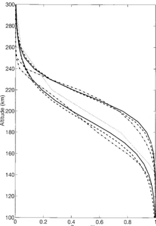
Figure 1 presents some empirical composition models for typical summer night and day conditions (see caption). The EISCAT model (not time dependent) is somehow an average between the night and the day IRI models. The

Fig. 1. Comparison between empirical composition models. Dotted

line: EISCAT time-independent model. Dash-dotted lines: IRI model

at midnight (below the EISCAT model) and at noon (above the EISCAT model). Dashed lines: Lathuille`re’s model. Solid lines: our model

transition region covers the domain in altitude: 140— 300 km and the transition altitude is 200 km. Lathuillere’s and our models are able to follow qualitatively the IRI profiles.

The ionospheric parametric model is formally written:

pN "fM (aN, rN),

where aN represents the vector formed by the coefficients of the polynomial models and the composition parameters to be fitted. As we saw, it is an empirical model which contains some physics in the implicit a priori knowledge on the ionospheric parameter profiles. This is the strength of the global regression technique. Nevertheless, we have to keep in mind that unrealistic implicit knowledge may give a wrongly fitted profile.

2.2 ACF model

Under standard assumptions of stationary and locally homogeneous plasma, the expectation value of the back-ground-noise-substracted ACFs can be written for lag index l and gate index g:

X(l, g)J:: dt dr Wl(t, r)

(rg#r)2R (tl#t, pN(rg#r)), (2)

where tl and rg are, respectively, the nominal lag and the weighted range (see Appendix A).

This formula contains all the relevant instrumental function effects through integration in the lag(t)—range(r) domain. The pulse shape and filter correction are included in the two-dimensional ambiguity function Wl. The term 1/(rg#r)2 denotes the decrease in the radar sensitivity with increasing range (soft target case after the azimuthal integration).

Information about local plasma parameters pN (r) is con-tained in the medium correlation function R(t, p_{N ). This} function is obtained from the theory of electrostatic fluc-tuation in a homogeneous unmagnetised Maxwellian plasma at thermal equilibrium. The justification of the use of this theory in the quasi-homogeneous case is beyond the scope of this paper.

2.2.1 Ambiguity functions

The derivation of the two-dimensional ambiguity function for ACF measurements is presented in the Appendix (see also Lehtinen, 1986). The direct use of two-dimensional functions for the evaluation of Eq. 2 is time-consuming. This operation can be simplified by making specific ap-proximations depending on the actual transmitted wave-form, correlator algorithm, filter bandwidth and signal spectral width. We shall now describe these approxima-tions for the EISCAT CP1.

The CP1 experiment contains four different data sets coming from different transmitted pulses: a 16-bit alter-nating-code for D- and E-region ion-line measurements, a long-pulse Gen system for F-region ion-line measure-ments and two power profiles. We will only be concerned with the first two modulations: the alternating-code which covers ranges from 89 to 277 km with 3.15-km range increments (i.e. a subpulse length of 21ls) and roughly the same range resolution — the 350-ls long-pulse Gen-system modulation which covers ranges from 150 to 600 km with a range increment of 22.4 km and a range resolution of 54 km. Given these experimental characteristics we can make the following approximations:

— Good height resolution

When the range resolution is short compared to the ionospheric scale height, we introduce in Eq. 2 the development: 1 (r#rg)2R(tl#t, pN(rg#r))+ 1 r2gR(tl#t, pN(rg)) #rdpi dr LR Lpi(tl#t, pN(rg))#O(r2).

This leads to the zero-order approximation of the ACF model:

X(l, g)J1/r2g : dtWtl(t)R(tl#t, pN(rg)), (3) where

Wtl(t)": drWl(t, r)

is the lag ambiguity function.

The zero-order approximation is equivalent to the standard hypothesis of a uniform plasma over the

scattering volume. In this case, only the filter and lag weighting effects are taken into account. First- and higher-order corrections depend on the shape of R and on the range resolution. The definition of rg is such that :drrWl(t, r)"0 (See Appendix A). This property en-sures that the first-order correction is small.

For the alternating-code, the range resolution (+3.15 km) is small enough to use the zero-order ap-proximation for most of the ionospheric state. This may be critical only if very short spatial lengths are encoun-tered, for example during electron precipitation. But, in such a case, the hypothesis of homogeneity in the direc-tion perpendicular to the beam behind the azimuthal integration leading to Eq. 2 may be wrong as well. The zero-order approximation can also be used for the long-pulse data taken above the F-region peak (typically 400 km), where the scale height becomes much greater than the range resolution.

— Long-pulse Gen-system in E and F regions

In the E and F regions, the range resolution of the long-pulse modulation is larger than the typical iono-spheric spatial scale. The zero-order Taylor develop-ment is no longer valid, and it is necessary to take into account the range smearing effect. The simplification now comes from the fact that the filter impulse response is much shorter than the pulse length. As pointed out by Holt et al. (1992), the two-dimensional ambiguity func-tion can be approximated by the product of the lag ambiguity function Wtl(l) and the range ambiguity function

Wrl(r)": dt Wl(t, r)/:: dt drWl(t, r).

The data model for long-pulse measurement becomes:

X(l, g)J:: dt dr R(tl#t, pN(rg#r))Wtl(t) Wrl(r)

(rg#r)2 . (4) For the CP1 long-pulse modulation, the maximum mean square error between the two-dimensional ambi-guity function and its factorised form Wtl(t)Wtl(r) is 0.3%. The effect of the ambiguity function approxima-tion on the data model is negligible compared with the typical standard deviation of the measurements.

2.3. Fitting procedure

An explicit parametric model of the measurement

X(l, g, a_{N ) is obtained by replacing the local plasma}

par-ameter pN (r) by the ionospheric model fM (aN, r) in one of the ACF models 2, 3 or 4, depending on the region of the ionosphere. The fitting procedure consists in the minimi-sation of the quadratic function:

F(aN )"+

g,l

DXK(g, l)!X(l, g, aN)D2

Var (X(l, g)) , (5)

where XK (g, l) is the measurement and Var(X(l, g)) its vari-ance.

In the frame of Gaussian statistics, the minimisation of

F(aN ) corresponds to the maximum likelihood estimate of

the parameter vector aN . The minimisation method we use

gives access to the parameter vector uncertainties as well as its optimum value. The discussion of the minimisation method is not the purpose of this paper.

3 Simulations

The simulations are intended to evaluate the statistical properties of the parametric inversion for the CP1 experi-ment. For the composition fitting strategy, only signals coming from the range between 107 and 433 km will be used.

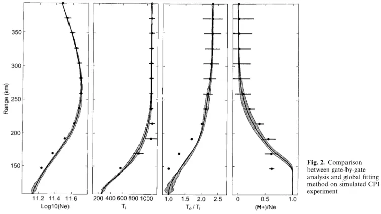
Figure 2 presents the ionospheric model used for the simulation of these gates. This model roughly corresponds to the ionosphere state on 4 August 1992 around noon. The solid lines, from left to right, are the profiles of log10(ne/n0), ti, tr and c. The velocity profile is set to zero during the simulations and is not presented on the figure; nor is the collision-frequency profile given by the standard analysis model. The simulation of build ACFs (result of lag-profile decoding) is performed using Eq. 2 and the ionospheric model of Fig. 2. In order to limit integration errors, the integration steps are eight times smaller than the inverse of the filter cut-off frequency. This is enough compared with the signal time and space frequency band-widths. The data variance is computed with a system noise temperature of 110°K and a transmitter power of 1.2 MW. Three points are discussed: the validity of approximate models (replacement of Eq. 2 by Eqs. 3 and 4), the statis-tical properties of the inverted composition parameters and the fit sensitivity to the ionospheric model.

3.1 Data model validation

The systematic bias of inverted parameters is addressed by fitting noiseless synthetic data with the approximate ACF models given by Eqs. 3 or 4. These models are computed with one-dimensional Riemann sums in the frequency-range domain rather than in the lag-frequency-range domain. The frequency domain is now limited to the filter bandwidth. For data model 4, the range step is roughly the alternat-ing-code range increment.

Model 3 (homogeneous plasma approximation) is tes-ted with gate-by-gate inversion (standard analysis). The dots in Fig. 2 represent the result of the long-pulse data inversion. Error bars correspond to $ the uncertainty on the inverted parameters for an integration period of 1 min. The result of the inversion for three or four lower gates are obviously biased compared to the plasma parameter of the simulation. The bias is much larger than the error bars. We cannot use the result of the fit of the long-pulse gates in the lower F region. The analysis method present-ed in Lathuillere et al. (1983b), which consists in adjusting the composition model on the fit result for the few gates in the transition region, is not possible in our case. In fact the Lathuillere et al. (1983b) method was applied to an ACF estimator (triangular weighting) different from that used in the present CP1 program (Gen weighting). It did not succeed to analyse the ACF measured with long-pulse Gen estimator (Lathuille`re, private communication).

Fig. 2. Comparison between gate-by-gate analysis and global fitting method on simulated CP1 experiment

Higher gates are less affected by the range smearing effect. For the long-pulse data of the CP1 experiment, Model 3 is valid only above the F-region peak.

Alternating-code fitted parameters (not presented in the figure) are very close to the parameter of the simula-tion. The uniform plasma approximation is accurate enough for this data set. Nevertheless, the uncertainty on the composition is so big that, in practice, the fit of the composition does not converge. Alternating-code gates cannot be used alone to measure the composition.

The global inversion is performed using data model 3 for the alternating-code gates and data model 4 for the long-pulse gates. The result of the inversion is represented by the grey areas drawn on Fig. 2. These areas correspond to the confidence interval at $ the uncertainty of the profile, still for an integration period of 1 min. We see that the areas are centred on the parameter of the simulation. There is no noticeable bias between the inverted profiles and the simulation profiles (see next section for a quanti-tative estimate). The approximate long-pulse data model is accurate enough. Outside the composition transition region the use of the physically constrained composition model gives a drastic gain on the other parameter uncer-tainties.

3.2 Composition parameter statistics

The two long-pulse gates below the transition altitude do not constrain enough our profile model in this zone. The parameters z50, dzc and Dz could not be fitted simulta-neously. We chose to fix Dz to 60 km, so that for the transition altitude 200 km there is no ion O` below

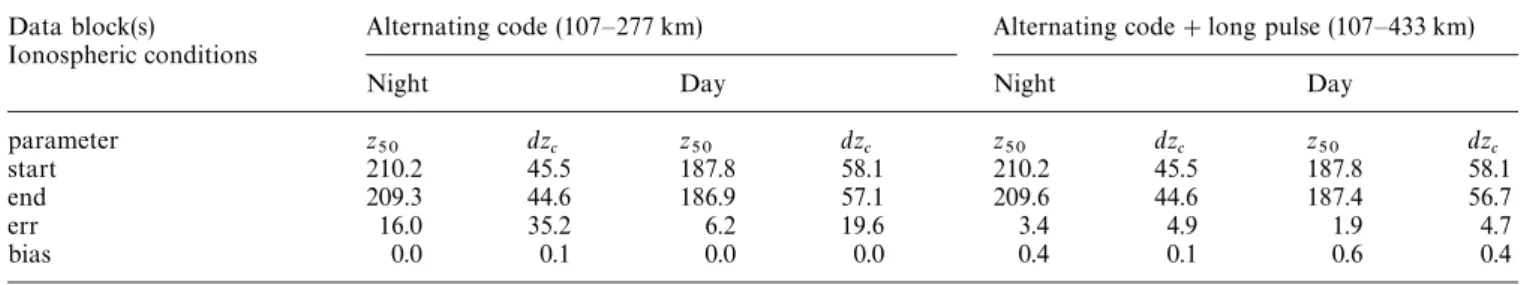
140 km. This arbitrary choice corresponds to the standard EISCAT composition model. The feasibility of accurate inversion of the two other parameters can be evaluated by looking at their uncertainties and bias. Table 1 presents the fit behaviour for two strategies: only alternating-code data are fitted, and alternating-code data are fitted to-gether with long-pulse data, and for two typical ionos-pheric conditions (night and day). In these simulations, the integration period is 5 min. For each fit condition, we give the starting values of the fit on the line labelled ‘‘start’’, the fit results on line ‘‘end’’, the standard deviation of the a posteriori distribution on line ‘‘err’’ and finally on line ‘‘bias’’ the difference between the end values and the simulation parameters.

With the experiment of only alternating code, we see that the uncertainty on dzc is of the same order as its value. It means that this parameter is hardly constrained. In practice the fit does not converge fast enough. The uncer-tainty on z50 is in the best case (day) 6 km. It is of the same order as the expected diurnal variation of this parameter (+25 km). The alternating-code experiment is obviously not adapted to composition fitting. The lack of constraint on composition parameters is certainly due to the relative-ly low SNR (small scattering volume). However, it is also due to the large lag increment (21ls) which does not give a good enough sampling of the ACFs, especially in its tail, where composition affects its shape. A 10-ls, 32-bit alter-nating code may be better in that sense even if the SNR is lower than for the 16 bit.

A way to solve this problem in the case of CP1-experi-ment data is to use the long-pulse data set. Indeed the corresponding modulation is characterised by a much higher SNR and a smaller lag increment (10ls) than the

Table 1. Statistical behaviour of the difficult parameter fit

Data block(s) Alternating code (107—277 km) Alternating code#long pulse (107—433 km) Ionospheric conditions

Night Day Night Day

parameter _{z50 dzc z50 dzc z50 dzc z50 dzc} start 210.2 45.5 187.8 58.1 210.2 45.5 187.8 58.1 end 209.3 44.6 186.9 57.1 209.6 44.6 187.4 56.7 err 16.0 35.2 6.2 19.6 3.4 4.9 1.9 4.7 bias 0.0 0.1 0.0 0.0 0.4 0.1 0.6 0.4

alternating-code modulation. Nevertheless, it is necessary to process alternating-code data at the same time. It is first needed to fix the bottom limit conditions on the iono-spheric classical parameters used in range deconvolution of the first long-pulse gate. It also allows to keep an acceptable range resolution of the density profile in the transition zone. Table 1 shows that in this case the uncer-tainties on dz are divided by 4 (day) and 7 (night), while uncertainties on z50 are divided by 3 (day) and 5 (night). It is now possible to fit the slope of the transition region and the track the diurnal variation of the transition altitude, at least during day. During night, the SNR diminution can be compensated by increasing the integration time up to 15 min.

Concerning the bias introduced by the use of approxi-mate ambiguity functions, we see that for these typical conditions, it stays below the parameter error. We con-sider that our data model is thus accurate enough for our purpose. Nevertheless if the systematic bias becomes a problem, exact ambiguity functions could be used. The statistical behaviour of the fitting procedure should any-way not be very much modified.

3.3 Ionospheric model sensitivity

The choice of the ionospheric model was taken to add as few constraints as possible on classical parameters and to use as few fitted parameters as possible to describe the composition profile. Indeed, the convergence of composi-tion parameter is in practice obtained only if two par-ameters or less are fitted. Uses of polynomials for difficult parameters were avoided because they are not suitable to describe asymptotic branches.

The sensitivity of the result to the model choice has been tested against the knot positions of the classical parameter profiles. Results were found to be independent of the knot positions when they are not closer than twice the alternating range increment. If not, numerical oscilla-tions spoil the profiles.

4 Application to actual data

We have used 133 h of CP1K data collected during the MLTCS (Mesosphere low-thermosphere coupling study) compaign starting on 30 July 1992 at 1600 and finishing on 5 August 1992 at 0500 (see EISCAT, 1992 for details).

The first 5 days are characterised by a rather low activity with an electric field lower than 10 mV m~1 during day and no more than 40 mV m~1 in the auroral oval. This first period is thus suitable for the inversion of composi-tion using the model of smooth temperature profiles. Intense electric field and precipitations were observed from the last evening (4 August 1992) up to the end to the experiment. This last period will be used to discuss the limitation of the method during disturbed ionospheric conditions.

4.1 Advanced calibration

When different data sets are fitted simultaneously, one needs a careful calibration in order to compensate for systematic differences in the estimation of the backscatter-ing cross-section. Identified sources for such technical problems are: non-constant receiver noise (receiver recov-ery and non-constant transmitted power (capacitor bank) during one transmitter cycle. A variation of the receiver noise introduces small error on the background noise estimate. After background substraction, a significant er-ror on the zero lag estimate occurs for low-SNR data, i.e. the two short-pulse power profiles of the CP1 experiment. This is not critical for the high-SNR long-pulse data. Alternating-code data are free from the noise power, and are not affected at all by this calibration problem. In order to avoid calibration problems, only these two last data sets were used.

A manual intercalibration of the long-pulse and alter-nating-code data was needed to adjust the two density profiles. The long-pulse system constant was multiplied by 1.17. This correction is of the same order as that used in the standard analysis. In the future we plan to perform an automatic intercalibration.

4.2 Daily variation of the composition

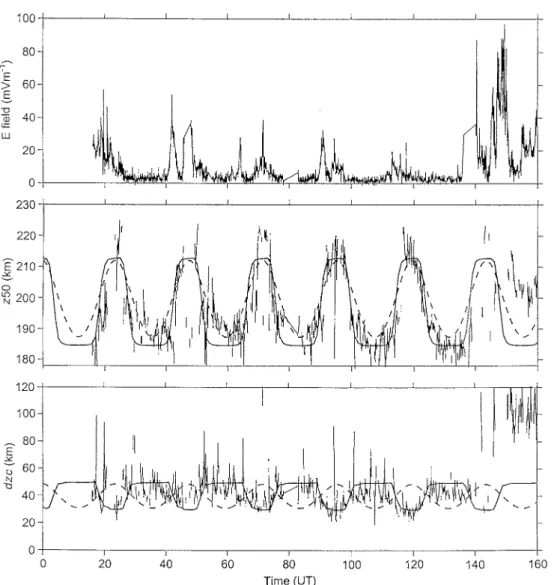
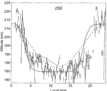
The inverted transition altitude and width of the transition region are plotted on the middle and bottom panels of Fig. 3. The time-scale is the elapsed time from 30 July 1992, 0000 UT. The dashed curves represent the daily empirical model of the transition altitude and scale height published in Lathuillere and Pibaret (1992). This empirical model has been obtained from data collected between October 1981 and August 1986 from CP0 and

Fig. 3. Transition altitude and transition width of the composition profile derived from the MLTCS campaign

CP1 experiments. The solid curves represent the composi-tion parameters obtained by fitting our model on the IRI composition profile. The top panel shows the electric field inferred from the tristatic Doppler velocity measurements. Looking at the period of electric field lower than 10 mV m~1, we see that our estimation of the altitude transition agrees fairly well with the IRI model. The tem-poral variation of Lathuille`re’s empirical model is smoother than what we have obtained. This may be due to a coarser time resolution (3 h) than the present one (15 min). The maximum of the transition altitude occurs around midnight, between the two passages of the auroral oval. The ionospheric activity associated with the auroral oval may contribute to some of the transient variations of the transition altitude around midnight. Nevertheless, the mean behaviour presented in Fig. 4 is still compatible with the IRI (solid line) and Lathuille`re’s (dashed line) empiri-cal models. On this figure, we estimate that the daily maximum of the transition altitude is approximately 215 km. A minimum of the transition altitude exists around noon near 185 km. From the same data, the same value was found by Shibata et al. (1995) with the method

of residual temperature profiles given by the standard analysis of the alternating-code gates. With this method, the transition altitude was not accessible between 2200 and 0400 due to low SNR. Therefore, the maximum of the transition altitude could not be compared with our es-timation.

Going back to Fig. 3, we see that the width of the transition region is of the same order as in Lathuille`re and Pibaret (1992). The difference with this earlier result is that we found a daily variation anticorrelated with the transition altitude, rather than correlated. Therefore, a comparison of the two methods with the same data set should be made. Yet our feeling is that the observed difference is certainly due the inversion method, i.e. either the data model or the composition model. We made an indirect check of the latter hypothesis by fitting both models on profiles got from the IRI composition model. In this case the composition parameters have the same evolution for both composition models. Therefore, the difference in the composition model is not responsible for the disagreement between the two methods. From Fig. 2, it is clear that the use of the data model 3 (homogeneous

Fig. 4. Daily variation of the transition altitude during quiet days

plasma approximation) introduces a systematic bias which could modify the estimation of the width of the transition region when using the method of Lathuille`re et

al. (1983b). Because the weighting was not the same as in

the simulation of Fig. 2, it is hard to tell how much the results are affected. Actually, the quality of the estimation of z50 and dzc was discussed in Lathuille`re et al. (1986). It was shown that z50 is correctly estimated, while dzc is on average underestimated. Moreover, the good agreement between our estimation of the width of the transition region obtained and the one obtained by fitting our com-position model on the IRI comcom-position model is a strong indication that our method gives a correct estimation of this parameter.

Non-daily modifications of the composition profile ap-pear during electric-field enhancements, at the instant of the auroral-oval passage and at the end of the experiment, during a major ionosphere disturbance (magnetospheric substorm). The interpretation of these modifications is beyond the scope of this paper. Indeed a careful validation of the global fitting method in presence of electric field and precipitation must be made above all. Qualitatively, we see that small drops in the transition altitude seem to be correlated with spikes in the electric fields, while a drastic change in the composition parameters occurs after the start of the substorm.

5 Conclusion

We have presented an application of the global fitting technique to EISCAT CP1 data for the inversion of the composition scale height and altitude transition. The vali-dation of the method was successfully made on a simulated experiment. It was shown that an accurate estimation of the composition parameters is possible only if high-resolution alternating-code gates are processed

together with lower-resolution but higher-SNR long-pulse gates. We do not expect significant improvement of the inversion either by using the power profiles and/or the covariance matrix of the measurements. Actually, the CP1 experiment may not be the best experiment for the com-position study: the alternating-code gates do not have a good enough sampling in the ACF tail, and the long-pulse gates are very much affected by the range smearing effect.

The application to an actual experiment and the comparison between different methods showed that the transition altitude behaviour is almost independent of the method used. The influence of the method on the behaviour of the width of the transition region is much more important. However, the careful treatment of the range smearing effect in our method and the good agreement between our results and the IRI model are indications of the validity of our method, at least during quiet periods. The large amount of available CP1 data allow the study of the seasonal variation of the composition.

The method is still to be tested during disturbed peri-ods, in the presence of electron precipitation and/or high electric field. In such a situation, the number and the position of the knots in the temperature profile will cer-tainly have to be modified. If the uncertainty does not increase too much, it will be possible to evaluate the ionospheric response to auroral precipitation.

Another perspective is to extend the method to the fit above the F-region peak. In this region, the H` concen-tration is easily determined. The global fitting technique may be used to address its velocity in order to study the polar wind.

Appendix A

Radar signal

This appendix present a possible way of deriving the expression of the scatter radar measurement. It is mainly intended to introduce explicitly the notations used in this paper. One may refer to Rino (1978) for the scattering process and to Lehtinen (1985) for the treatment of the two-dimensional ambiguity function.

The derivation of the radar signal is carried out in the general case of a transmitter situated at point r_{l 0 and a receiver situated} at point r_{l 1. Index 0 will refer to the transmitter and index 1 to} the receiver. Let x(t) be the RF complex signal at the receiver input; x(t) is the sum of a Gaussian noise xn(t) and the scattering signal:

xs(t)Jexp(ju0t) : drlds(rl, t)A(t!(R0(rl)#R1(rl))/c)

]

S

4nR20(rl)

S

The purpose of the scatter experiment is to perform a spectral analysis in the ql domain of the succeptibility fluctuation ds(rl, t). In our case it is a stationary Gaussian random process, all the information is contained in the correlation function Sxs(t@)xs(t)T. After demodulation and filtering of xs(t), a common procedure consists of estimating the expectation value of lagged products of the

signal x(t) (we do not consider the noise contribution):

Xtt{"Sx*(t)x(t@)T

J_{exp( j}Du(t@!t)) :::: dl dl@ drl drl @ Sds(rl, t)ds(rl @, t@)T ]exp( j(Du(l@!l))

]p(l)p(l@)A*(t!l!¹(rl))A(t@!l@!¹(rl @))

]U*(rl, t!l)U(rl @, t@!l@)exp(!j(u(rl @)!u(rl))), (7) whereDu"u1!u0, p(l) is the filter impulse response and: ¹(rl )"(R0(rl)#R1(rl))/c,

U(rl )"

S

4nR20(rl)

S

Equation 7 can be simplified under the assumption of short correc-tion length ofds(rl, t) compared to spatial variations of the propaga-tion delay ¹(r_{l ) and the illumination profile U(r). Introducing the} slow and fast variables Rl"(r_{l @#rl )/2 and oN"rl @!rl @, one may use} the zero-order developments:

¹(rl )+¹(rl @)+¹(Rl), U(rl )+U(rl @)+U(Rl),

and in the limit of far field zone the first-order development: u(rl @)!u(rl)+( +lu)Rool.

Using these approximations and the definition of the local spectral density (locally homogeneous approximation):

Ss(ql, q, Rl)": dolSs(Rl!ol/2, 0)s(Rl#ol/2, q)T exp(jql·ol), (8) Eq. 7 becomes (q"l@!l):

Xtt{Jexp ( jDu(t@!t))

]:: dr dRlSs((+lu)Rl,q, Rl) exp(jDuq)DU(Rl)D2

][: dlp(l)p(l#q)A*(t!l!¹(Rl))

]A(t@!l!l!¹(Rl))]. (9) This expression contains the receiver bandwidth effect and the range smearing effect through the integration overq and Rl. The integral under brackets represents the two-dimensional ambiguity function in lagq and propagation delay ¹ domain, which will be denoted hereafter Wtt{(q, ¹), Ss((+lu)Rl,q, Rl) is the quantity of interest, i.e. the

local spectral density taken at local wave vector ql (Rl)"(+oou)Rl.

Practical estimation of Ss is usually made by computing a weighted sum of lagged products for t@!t constant and coming from the same pulse or different ones. This operation, referred to as lag profile sampling and filtering, depends on the transmission modulation and the correlator algorithm. Any sample i of the background subtracted correlator output is written as (q"t@!t):

XiJexp (jDuqi) :: dq dRlSs(ql(Rl), q, Rl)

]exp (jDuq)DU(Rl)D2Wi(q, ¹(Rl)), (10) where the weighted ambiguity function Wi is formally:

Wi(q, ¹ )"+Ni

k/1w(i,k)Wtk,tk`q(q, ¹),

(11) andu(i,k) are the weighting factors of cross-product k in sample i.

When working with build ACF we prefer to use the lag index

l and the gate index g rather than the sample index i, and to use the

centred ambiguity function: Wl(q, r)"Wi(q!g, (r!rg)/c), whereql"qi is the nominal lag and

rg"Sc : ¹ d¹ dq Wi(q, ¹ )/:d¹ dqWi (q, ¹ )Tl

is the weighted range for the gate g. With these notations, the ambiguity function Wl(q, r) is now independent of the gate index.

Application to incoherent-scatter radar

Equation 10 may be simplified for the particular case of an ion line experiment (Du"0) and monostatic geometry (¹(Ro)" 2DRlD/c"2r/c). Assuming a broad ql spectrum for Ss, one may be neglected the finite instrumental resolution, i.e. one may use a con-stant instrumental wave vector q_{l over the scattering volume:}

q_{l (Rl)"2kul"ql,}

with u_{l the unit vector of the radar beam oriented toward the} antenna.

For thermal fluctuations, the susceptibility correlation is:

Ss(ql, q, Rl)JR(q, pN(Rl)), (12) where R is the plasma density fluctuation correlation function for the spatial wave vector ql ; R is given by the theory of plasma density thermal fluctuations and pN represents the plasma parameters on which R depends.

Finally, neglecting transverse gradients of p_{N , the azimuthal} integ-ration of Eq. 10 and using the lag-gate sample indexation we obtain:

X(l, g)J:: dq dr Wl(q, r)

(rg#r)2R(g#q, pN(rg#r)). (13)

Acknowledgements. We thank Chantal Lathuille`re for fruitful

dis-cussions and providing interesting materials. We thank the referees for their constructive comments. We also would like to thank the EISCAT Scientific Association for providing Common-Program data. EISCAT is an international facility supported by the research councils of Finland, France, Germany, Norway, Sweden and the U.K. Bertrand Cabrit’s work was supported by a grant from the Socie´te´ de Secours des Amis des Sciences.

References

Dougherty, J. P., and D. T. Farley, A theory of incoherent scattering of radio waves by a plasma, Proc. R. Soc., A259, 79—99, 1960.

EISCA¹ annual report, EISCAT Scientific Association, 1992.

Evans, J. V., Theory and practice of ionosphere study by Thomson scatter radar, IEEE Proc. IEEE, 57, pp. 496—530, April 1969. Hagfors, T., Density fluctuations in a plasma in a magnetic field,

with applications to the ionosphere, J. Geophys. Res., 66, 1699—1712, 1961.

Holt, J. M., D. A. Rhoda, D. Tetelbaum, and A. P. Van Eyken, Optical analysis of incoherent scatter radar data, Radio Sci., 27, 345—348, 1992.

Kelly, J., and V. B. Wickwar, Radar measurements of high-latitude ion composition between 140 and 300-km altitude, J. Geophys.

Res., 86, 7617—7626, 1981.

Kofman, W., and C. Lathuille`re, EISCAT multipulse technique and its contribution to auroral ionosphere and thermosphere descrip-tion, J. Geophys. Res., 90, 3520—3524, 1985.

Lathillue`re, C., and B. Pibaret, A statistical model of ion composi-tion in the auroral lower F region, Adv. Space Res., 12, 146—156, 1992.

Lathuille`re, C., V. B. Wickwar, and W. Kofman, Incoherent scatter measurements of ion-neutral collision frequencies and temper-atures in the lower thermosphere of the auroral region, J.

Geo-phys. Res., 88, 10137—10144, 1983a.

Lathuille`re, C., G. Lejeune, and W. Kofman, Direct measurements of ion composition with EISCAT in the high-latitude F1 region,

Radio Sci., 18, 887—893, 1983b.

Lathuille`re, C., W. Kofman, and Pibaret, Incoherent scatter measure-ments in the F1 region. J. Atmos. ¹err. Phys., 48, 857—866, 1986. Lehtinen, M. S., Statistical theory of incoherent scatter radar

measurements, ¹echnical note 86/45, EISCAT scientific associ-ation, S-98127 Kiruna, Sweden, June 1986.

Oliver, W. L., Incoherent scatter radar studies of the daytime middle thermosphere, Ann. Geophysicae, 35, 121—139, 1979.

Rino, C. L., Incoherent scatter radar signal processing techniques, ¹echnical memo, SRI international, 333 Ravenswood avenue, Menlo Park, California 94025, USA, March 1978.

Salpeter, E. E., Electron density fluctuation in a plasma, Phys. Rep., 120, 1528—1535, 1960.

Shibata, T., K. Inue, and C. Schlegel, Ion composition in the lower F region inferred from residual of ion temperature profile mea-sured with the EISCAT CP1 experiment, J. Geomagn. Geoelectr., 47, 879—888, 1995.