HAL Id: insu-03006719
https://hal-insu.archives-ouvertes.fr/insu-03006719
Submitted on 16 Nov 2020
HAL is a multi-disciplinary open access
archive for the deposit and dissemination of sci-entific research documents, whether they are pub-lished or not. The documents may come from teaching and research institutions in France or abroad, or from public or private research centers.
L’archive ouverte pluridisciplinaire HAL, est destinée au dépôt et à la diffusion de documents scientifiques de niveau recherche, publiés ou non, émanant des établissements d’enseignement et de recherche français ou étrangers, des laboratoires publics ou privés.
The Philae lander reveals low-strength primitive ice
inside cometary boulders
Laurence O’rourke, Philip Heinisch, Jürgen Blum, Sonia Fornasier, Gianrico
Filacchione, Hong van Hoang, Mauro Ciarniello, Andrea Raponi, Bastian
Gundlach, Rafael Andrés Blasco, et al.
To cite this version:
Laurence O’rourke, Philip Heinisch, Jürgen Blum, Sonia Fornasier, Gianrico Filacchione, et al.. The Philae lander reveals low-strength primitive ice inside cometary boulders. Nature, Nature Publishing Group, 2020, 586 (7831), pp.697-701. �10.1038/s41586-020-2834-3�. �insu-03006719�
The Philae lander reveals low strength primitive ice inside cometary boulders
Laurence O'Rourke1*, Philip Heinisch2, Jürgen Blum2, Sonia Fornasier34, Gianrico Filacchione5, Hong
Van Hoang36, Mauro Ciarniello5, Andrea Raponi5, Bastian Gundlach2, Rafael Andres7, Bjoern Grieger8,
Karl-Heinz Glassmeier2, Michael Küppers1, Alessandra Rotundi95, Olivier Groussin10, Dominique
Bockelée-Morvan3, Hans-Ulrich Auster2, Nilda Oklay11, Gerhard Paar12, Maria del Pilar Caballo
Perucha12, Gabor Kovacs13, Laurent Jorda10, Jean Baptiste Vincent14, Fabrizio Capaccioni5, Nicolas
Biver3, Joel Parker15, Cecilia Tubiana16, Holger Sierks16.
1 European Space Astronomy Centre, European Space Agency, Urbanización Villafranca del Castillo,
Villanueva de la Cañada, 28692, Madrid, Spain
2 Institut für Geophysik und extraterrestrische Physik, Technische Universität Braunschweig,
Mendelssohnstr. 3, 38106 Braunschweig, Germany
3 LESIA, Observatoire de Paris, Université PSL, CNRS, Université de Paris, Sorbonne Université, 5 place
Jules Janssen, 92195 Meudon, France
4 Institut Universitaire de France (IUF), 1 rue Descartes, 75231 PARIS Cedex 05 5 INAF-IAPS, Institute for Space Astrophysics and Planetology, Rome, Italy
6 Université Grenoble Alpes, CNRS, Institut de Planétologie et Astrophysique de Grenoble (IPAG), UMR
5274, Grenoble F-38041, France
7 Telespazio Vega UK Ltd. for ESA/ESAC, Urbanización Villafranca del Castillo, Villanueva de la
Cañada, E-28692, Madrid, Spain
8 Aurora Technology B.V. for ESA/ESAC, Urbanización Villafranca del Castillo, Villanueva de la
Cañada, E-28692, Madrid, Spain
9 Universitá degli Studi di Napoli Parthenope, Dip. di Scienze e Tecnologie, CDN IC4, I-80143 Naples,
Italy
10 Aix Marseille Univ, CNRS, CNES, LAM, Laboratoire d’Astrophysique de Marseille, Marseille, France 11 Independent Contributor, Berlin, Germany
12 JOANNEUM RESEARCH Forschungsgesellschaft mbH, Steyrergasse 17, 8010 Graz, Austria 13 Budapest University of Technology and Economics, Department of Mechatronics, Optics and
Engineering Informatics, Bertalan L. str. 4, 1111 Budapest, Hungary
14 DLR, Institute of Planetary Research. Extrasolar Planets and Atmospheres, Rutherfordstraße 2, 12489
Berlin, Germany
15 Southwest Research Institute (SwRI), Planetary Science Directorate, Suite 300, 1050 Walnut Street,
Boulder, CO 80302-5150, U.S.A.
16 Max-Planck-Institut für Sonnensystemforschung, Justus-von-Liebig-Weg, 3, 37077, Göttingen,
Germany
ABSTRACT
On the 12th November 2014, the Philae lander descended towards comet 67P/Churyumov-Gerasimenko rebounding off the surface, colliding, then rebounding one last time before arriving under a cliff in the Abydos region. The landing process provided new insights on the properties of a cometary nucleus1,2,3. Here we report on the previously
undiscovered second rebound touchdown site where Philae spent almost 2 minutes of its cross-comet journey producing four distinct surface contacts on two adjoining cometary boulders. It exposed primitive water ice in their interiors while travelling through a crevice between the boulders. Our multi-instrument observations made 19 months later find the water ice mixed with ubiquitous dark organic-rich material has a local dust/ice mass ratio of 2.3+0.2
-0.16 : 1 matching values previously found in newly exposed water ice from
outbursts4 and water ice in shadow5,6. At the end of the crevice, Philae made a 0.25m deep
impression in the boulder ice providing in-situ measurements confirming primitive ice has a very low compressive strength (< 12Pa) as well as allowing a key estimation (75±7%) to be made for the porosity of the boulders’ icy interiors. Our results provide important constraints for cometary landers seeking access to a volatile rich ice sample.
MAIN TEXT
Flybys and rendezvous missions have been key to providing close up images of cometary surface structures delivering important insights into the chemical and physical processes that have defined them7. The presence of boulders on their surfaces with sizes
ranging from the metre scale up to 10s of metres often in locations not matching where they were initially exposed certainly points to the dynamic nature of their creation8,9. A
determination of mechanical strength properties derived from in-situ measurements carried out on the primitive ice located in the interior of a cometary boulder allows unique comparisons to be made with the cometary body internal structure. Furthermore, it provides insights on its dynamical history and delivers important constraints for the design of cometary landers and cryogenic sample return missions.
The European Space Agency’s Rosetta mission10 was launched in 2004 and began
orbiting comet 67P/Churyumov-Gerasimenko in August 2014. On 12th November 2014
the Philae lander was released with a faulty harpoon system, touching down on the surface on two occasions while also experiencing a glancing collision against the Hatmehit depression edge. After Touchdown 2 (TD2), it proceeded to its final position at Touchdown 3 (TD3) located under an overhang in the Abydos region of the comet1 (see
Fig. 1a-d). While scientific analysis of data1,2,11 from Philae’s first and third touchdown
points have ledto a significant step in understanding the properties of a cometary nucleus, the location and scientific implications stemming from the second touchdown point were unknown up to now. Its importance was noted12 however as Philae was found to have
with the Rosetta Lander Magnetometer and Plasma Monitor13 (ROMAP) sensor, possibly
exposing ice at the same time.
The production of a new Philae landing trajectory (Supplementary Methods, Supplementary Fig. 1) served to kick-off the search for the touchdown 2 point with a ridge region identified as being a likely candidate for its location11. A comparative
analysis was performed of this area using pre- and post-landing imagery (Supplementary Fig. 2 & 4) from the ROSETTA Optical, Spectroscopic, and Infrared Remote Imaging System (OSIRIS)14 combined with high resolution digital terrain models of the ridge e.g.
Supplementary Fig. 9-11, and the Abydos region as a whole. While significant changes in boulder positions were observed in the Abydos valley (Supplementary Fig. 4e and f), the geomorphological structures along the length of the ridge showed no differences with regards to position or orientation. Changes were found however in the pre- and post-landing surface morphology of two adjoining boulders located on the ridge (Extended data Fig. 1, Supplementary Video 1, Supplementary Fig. 5 & 6). These changes included the identification of an unusual ice feature located in the boundary between them (Fig. 1e, 1f, Supplementary Video 2). Our analysis of these changes found that only Philae’s presence could explain their existence (Supplementary Methods). As the topological structures of these two boulders, viewed from above, give the impression of a skull face as shown in Supplementary Fig. 3, we chose to name the location as skull-top ridge and the boundary between the two boulders as skull-top crevice. We highlight in Methods that the boulders’ themselves represent assemblages of dust/ice aggregates.
The timing involved in this chain of events [Extended Data Table 1, Supplementary Video 3] was derived from magnetometer data produced by the
ROMAP sensor and checked against thermal & power information from Philae’s subsystems. The ROMAP instrument provided attitude information (combined with the Rosetta Plasma Consortium Fluxgate Magnetometer (RPC-MAG)15) as well as unique
accelerometer measurements based upon sensor boom movement (see Methods). Combined with our image analysis, a reassessment of the ROMAP science data (see Methods and Supplementary Methods) determined that the initial contact took place at 17:23:48±10s, approximately 1.5 minutes before the previously published contact time16.
Indeed Philae spent nearly two full minutes at Touchdown 2 (TD2) making four surface contacts in its trip across it (see Supplementary Fig. 6). Of the four, the third (TD2c) of these contacts (Fig. 2) is the most significant due to the 0.25m deep depression visible in an ice-like feature on the side of the crevice. We found a perfect correlation between the presence of that depression and ROMAP boom movements (Fig. 2a) that show the expected deviations matching the stamping movement required for its creation. The compression lasted 3 seconds (Fig. 2b and c) before Philae proceeded to rise out of the crevice to then make its final TD2 contact with the surface (TD2d) creating the eye of the skull in the process.
Data from the OSIRIS and VIRTIS instruments on the Rosetta orbiter were used to determine whether the high albedo ice-like features observed in the skull-top crevice were water ice. For the OSIRIS instrument, we focussed on multi-filter images generated during the timeframe of 12th to 14th June 2016 (Fig. 3a, Extended Data Fig. 2). A
spectrophotometric analysis of the datasets from this period (see Methods) provided spatially resolved data that confirmed the presence of water ice in the crevice, matching a visible area of approximately 3.5 m2, with a brightness 6 times greater than the dust
corrections were made for the illumination conditions and phase function based upon geographical mixtures of the comet dark terrain and water ice (grain size of 30-100 microns) applied to the bright material absolute reflectance21. A water ice abundance
value of 46.4 +/- 2.0% was measured during the 14th June 2016 10:30 observations (Fig.
3c & d, Extended Data Table 1), resulting in an approximate local volume dust/ice ratio of 1.15+0.1-0.08 : 1. Assuming a dust/ice bulk density ratio of two17, and a similar porosity
for dust and ice material, the local dust/ice mass ratio is approximately 2.3+0.2
-0.16 : 1. This
value is below the average dust/ice mass ratio for the nucleus which is >3 for most estimates derived from measured data18.
A less sensitive result using data from the VIRTIS Instrument on the 14th June
2016 confirmed this detection of water ice. Fig. 3b shows the resulting hyperspectral image of the Abydos region with the skull-face crevice identified at the edge of the field of view. A signal from the ice located in the crevice was found in the tail of the optical point spread function (see Methods). An estimation by VIRTIS of the water ice abundance in the location concurred with that of the OSIRIS measurement whereby the water ice rich spot was determined to have an approximate area of 1.27 ± 0.5m2
(matching the upper bound of 48% of 3.5m2) calculated from the inferred abundances
(0.5% over an area of 253m2).
The general longevity of ice on the comet surface is dependent on local surface topography6,19,20,21 with most ice features disappearing quite quickly due to limited
surface shading from the sun within days to weeks of discovery. Local dust/ice ratios < 3:1 equivalent to that in the skull-top crevice have been found at other locations across the comet (as well as on other comets7,22), in particular in newly exposed water ice
observed on cliffs and scarps linked in some cases to outbursts as well as in clustered bright spots in both hemispheres4,6,21.As dust/ice ratios have been found to reduce over
time due to solar illumination exposure, the fact that our measurement of high water ice abundance was made 19 months post-landing and that the ice in the crevice was observed 22 months post-landing without significant measurable changes, both point to the ice in the crevice receiving very low sun illumination due to shadowing.
We confirmed this using a horizon mask (Extended Data Fig. 3) determining that the ice on the left hand side of the crevice was illuminated <0.55% of the time during the perihelion passage while the ice on the right hand side of the crevice, where the compression took place, received <0.21% of direct sunlight during the same period. Using as input the corresponding energy flux, we found our sublimation modelling over-estimated by an order of magnitude the amount of ice that sublimed (than is visible from the imagery) pointing to even greater morphological shadowing than our horizon mask could derive (Supplementary Methods). This very low illumination is supported by our direct measurements of the crevice dimensions; the width of the TD2c location fully matches the width of the Philae lander thus pointing to very little sublimation or erosion having taken place (Fig. 3e-e1). For these reasons, we conclude that while the super-volatiles may have sublimated over time, the water ice itself at TD2c did not sublimate and remained in a highly unprocessed state.
The depth of the impression made by Philae in this icy surface combined with a detailed correlation of the ROMAP boom measurements contribute to provide direct in-situ measurements allowing an estimation to be made of the compressive strength of this dust/ice feature. The depth of the impression in the ice is 0.246 ± 0.049 m (Fig. 3e-e2)
and its area is ≥ 0.2208 m2 (see methods). A detailed analysis performed and explained
in Methods, finds the compressive strength of the ice to be <12Pa. It is important to flag that this very low compressive strength is of “primitive” ice (see Supplementary Methods for explanation) buried and hidden from view until it was exposed and compressed at the time of the Philae landing itself.
While compressive strengths1,2 of 1kPa and 2MPa were measured at TD1 and TD3
respectively (although deployment uncertainties do affect the reliability of the MUPUS result), a number of other publications find much lower values. Model dependent analyses of the collapse of cliff overhangs observed from orbit23 as well as those derived from the
scratches Philae made at the final landing location11 calculated compressive strength
values ranging between 30 Pa and 150 Pa for the former and from 10 to 100Pa for the latter. Such model-based low compressive strength derivations show consistency with our in-situ findings.
Three independent porosity estimations have been made for this comet with values ranging from 65-85% (Philae Consert radar3,24), through 70-75% (Rosetta Radio
science Instrument) 25 and a modelled third estimate26 of 63-79%. These same numbers
equate to volume filling factors of 0.15-0.35, 0.25-0.3 and 0.21-0.37 respectively. We modelled the compression Philae made in the cometary boulder material, with the aim of determining how much the volume-filling factor of the material is altered. The model we use27 assumes that the material making up the cometary interior is made up of
a hierarchical arrangement of building blocks (see Supplementary Methods). According to this model, applied for the case of this paper to the interior of a cometary boulder, the
sub-µm-sized solid grains28,29 are contained in larger units ("pebbles"), which themselves
are clustered together to make up the boulder.
We find that such an arrangement of hierarchical building blocks, which previously has demonstrated excellent correlation with the Philae Consert radar results24,
also provides the conditions needed to achieve the low compressive strength (<12 Pa) of the material of the boulder into which Philae stamped (see Methods). We further note that although the local dust/ice ratio we measured (2.3+0.2
-0.16) is lower than the model based
average30 estimate of the nucleus (between 3 and 9), we can resolve this inconsistency. A
study of results from gas activity models31,32 (based also on our hierarchical pebble
model) explains our finding in that dust/ice ratios of 5 and lower can be found to be present locally for up to 5% of the volume of the nucleus29. As a result and on the basis
of the consistencies found using our model, we derive a volume filling factor for the boulder material of 0.25 ± 0.07, (porosity range of 68-82%) equivalent to previously published values for the overall nucleus of comet 67P.
Our results provide important constraints for future cometary lander missions as the knowledge of cometary boulder interiors is not only key for impact analysis but also provides insights for the mechanical processes needed to retrieve a volatile rich cryogenic sample for in-situ analysis or indeed for delivery back to the Earth33,34. The operational
dangers of landing in a cometary boulder field would need careful study and preparation however.
REFERENCES
1. Biele, J. et al., The landing(s) of Philae and inferences about comet surface mechanical properties, Science, 349, 6247, 2015.acc
2. Spohn, T. et al., Thermal and mechanical properties of the near-surface layers of comet 67P/Churyumov-Gerasimenko, Science, 349, 6247, 2015
3. Kofman, W., Herique, A., Barbin, Y., et al., Properties of the 67P/Churyumov-Gerasimenko interior revealed by CONSERT radar, Science, 349, 2015
4. Pajola, M. et al. The pristine interior of comet 67P revealed by the combined Aswan outburst and cliff collapse. Nat. Astron. 1, 0092 2017.
5. Fornasier, S. et al., Surface evolution of the Anhur region on comet 67P/Churyumov-Gerasimenko from high-resolution OSIRIS images, A&A, 630, A13, 2019
6. Oklay, N. et al, Long-term survival of surface water ice on comet 67P, MNRAS 469, S582–S597, 2017
7. Oklay, N. et al, Comparative study of water ice exposures on cometary nuclei using multispectral imaging data, MNRAS, 462, S394-S414, 2016
8. Luccheti, A. et al, Characterization of the Abydos region through OSIRIS high-resolution images in support of CIVA measurements, A&A 585, L1, 2016
9. Keller, H.U. et al, Seasonal Mass Transfer on the Nucleus of Comet 67P/ Chuyumov-Gerasimenko, MNRAS, 469, Issue Suppl_2, p.S357-S371, 2017
10. Glassmeier, K. et al. The Rosetta Mission: Flying Towards the Origin of the Solar System. Space Sci Rev 128, 1–21, 2007
11. Heinisch, P. et al., Compressive strength of comet 67P/Churyumov–Gerasimenko derived from Philae surface contacts, A&A, 630, A2, 2019
12. Heinisch, P. et al, Reconstruction of the flight and attitude of Rosetta's lander Philae, Acta Astronautica, 140, 509-516, 2017
13. Auster, H.U., et al. ROMAP: Rosetta Magnetometer and Plasma Monitor. Space Sci Rev 128, 221–240 2007
14. Keller, H., U., et al., OSIRIS – The Scientific Camera System Onboard Rosetta, Space Sci Rev 128, 433-506, 2007
15. Glassmeier, K., et al. RPC-MAG, The Fluxgate Magnetometer in the ROSETTA Plasma Consortium. Space Sci Rev 128, 649–670, 2007
16. Auster, H.U., et al., The non-magnetic nucleus of comet 67p/Churyumov– Gerasimenko, Science 349, 6247, 2015
17. Fulle, M., et al, The dust-to-ices ratio in comets and Kuiper belt objects, MNRAS, 469, S45, 2017
18. Choukroun, M., et al., Dust-to-Gas and Refractory-to-Ice Mass Ratios of Comet 67P/Churyumov-Gerasimenko from Rosetta Observations, Space Science Reviews, 216, pp.1-38, 2020
19. Deshapriya, J. D. P., Exposed bright features on the comet 67P/Churyumov– Gerasimenko: distribution and evolution
20. Filacchione G., et al., Exposed water ice on the nucleus of comet 67P/Churyumov-Gerasimenko, Nature, 529, 368-372, 2016
21. Fornasier, S., et al., Rosetta’s comet 67P/Churyumov-Gerasimenko sheds its dusty mantle to reveal its icy nature, Science, 354, 1566-1570, 2016.
22. Sunshine, J. M., et al. Exposed Water Ice Deposits on the Surface of Comet 9P/Tempel 1. Science 311, 1453 (2006)
23. Groussin, O., et al., Gravitational slopes, geomorphology, and material strengths of the nucleus of comet 67P/Churyumov-Gerasimenko from OSIRIS observations, A&A, 583, A32, 2015
24. Herique, A., et al. Homogeneity of 67P/Churyumov-Gerasimenko as seen by CONSERT: implication on composition and formation, A&A, 630, A6, 2019
25. Pätzold, M., Andert, T., Hahn, M., et al. A homogeneous nucleus for comet 67P/Churyumov–Gerasimenko from its gravity field, Nature, 530, 63, 2016
26. Fulle, M., Della Corte, V., Rotundi, A., et al. Comet 67P/Churyumov–Gerasimenko preserved the pebbles that formed planetesimals, Monthly Notices of the Royal Astronomical Society, 462, S132, 2016
27. Blum, J., et al, The Physics of Protoplanetesimal Dust Agglomerates. I. Mechanical Properties and Relations to Primitive Bodies in the Solar System, APJ, 652, 2, 1768-1781, 2006
28. Mannel et al. Dust of comet 67P/Churyumov-Gerasimenko collected by Rosetta/MIDAS: classification and extension to the nanometre scale, A&A, 630, A26, 2019
29. Güttler, C., et al. Synthesis of the morphological description of cometary dust at comet 67P/Churyumov-Gerasimenko, A&A, 630, A24, 2019
30. Lorek, S., Gundlach, B., Lacerda P., Blum J., Comet formation in collapsing pebble clouds - What cometary bulk density implies for the cloud mass and dust-to-ice ratio, A&A, 587, A128, 2016
31. Fulle, M. Blum, J., Rotundi, A., Gundlach, B., Güttler, C., Zakharov, V., How comets work: nucleus erosion versus dehydration, MNRAS 493, 4039, 2020
32. Gundlach, B., Fulle, M., Blum, J., On the activity of comets: understanding the gas and dust emission from comet 67P/Churyumov-Gerasimenko’s south-pole region during perihelion, MNRAS 493, 3690-3715, 2020
33. Ambition -- Comet Nucleus Cryogenic Sample Return; https://www.cosmos.esa.int/web/voyage-2050/white-papers
34. Cryogenic Comet Nucleus Sample Return (CNSR) Mission Technology Study : https://solarsystem.nasa.gov/studies/228/cryogenic-comet-nucleus-sample-return-cnsr-mission-technology-study/
ACKNOWLEDGEMENTS
B.G and J.B. thank the Deutsches Zentrium für Luft- und Raumfahrt (DLR) for continuous support and the Deutsche Forschungsgemeinschaft for their support under grant Bl 298/24-2 in the framework of the Research Unit FOR 2285 “Debris Disks in Planetary Systems”. OSIRIS was built by a consortium led by the Max-Planck-Institut fur Sonnensystemforschung, Goettingen, Germany, in collaboration with CISAS, University of Padova, Italy, the Laboratoire d'Astrophysique de Marseille, France, the Instituto de Astrofisica de Andalucia, CSIC, Granada, Spain, the Scientific Support Office of the European Space Agency, Noordwijk, The Netherlands, the Instituto Nacional de Tecnica Aeroespacial, Madrid, Spain, the Universidad Politechnica de Madrid, Spain, the Department of Physics and Astronomy of Uppsala University, Sweden, and the Institut fur Datentechnik und Kommunikationsnetze der Technischen Universitat Braunschweig, Germany. The support of the national funding agencies of Germany (DLR), France (CNES), Italy (ASI), Spain (MEC), Sweden (SNSB), and the ESA Technical Directorate is gratefully acknowledged. Those authors part of the VIRTIS and GIADA teams wish to thank the Italian Space Agency (ASI, Italy) contract no. I/024/12/2 and Centre National d’Etudes Spatiales (CNES, France) for supporting their contribution. The contribution of the ROMAP and RPC-MAG teams was financially supported by the German Ministerium für Wirtschaft und Energie and the Deutsches Zentrum für Luft- und Raumfahrt under contract 50QP1401. This research has made use of the scientific software shapeViewer (www.comet-toolbox.com). Video rendering was powered by PRo3D, a viewer for the exploration and analysis of planetary and smaller body surface reconstructions. It was developed by VRVis Zentrum für Virtual Reality und Visualisierung Forschungs-GmbH in close collaboration with JOANNEUM
RESEARCH and Imperial College London. Please see http://pro3d.space for more details. Trajectory and instrumental information relevant to the observations performed on Rosetta were based on the use of SPICE kernels. We acknowledge the important role played by the Rosetta Science Ground Segment, the Rosetta Mission Operations Team, the Philae Lander team(s) in the running of the Rosetta mission and Philae Lander Operations.
Author Contributions
Identification of the skull-top crevice ice and other touchdown points made by LOR. Paper Lead writer is LOR. Contributions to methods & supplementary sections was performed by LOR, PH, SF, HVH, GF, AR, MC, JB, BGu, AR, MdPCP & GP. The ROMAP & RPC-MAG data analysis performed by PH, KHG & UA. The compressive strength & porosity analysis was performed by JB & BG. The OSIRIS image analysis was performed by LOR, SF & HVH. The VIRTIS data analysis was carried out by GF, AR, MC & FC. The Skull-top crevice Ice & dust analysis carried out by AR, DB, MK, OG, NO. The OSIRIS Image processing was performed by SF, HVH, GK, CT & HS. Trajectory data analysis was performed by BGr, LOR, RA, PH, JBV, CT & HS. The Shape model support and analysis given by LJ, JBV, RA, MdPCP & GP. Figures (in support of analysis) generated by LOR, PH, RA, JB, BGu, SF, HVH, GF, AR & MC. All authors have participated in the review of the paper & its contents.
Data Availability
All OSIRIS, VIRTIS, RPC-MAG and ROMAP calibrated data are publicly available through the European Space Agency’s Planetary Science Archive website (https://archives.esac.esa.int/psa/). Significant effort has been spent in populating the Supplementary Methods and Supplementary Information document with additional supporting images, data and explanatory text with the aim to allow readers to be understand what we have done and how we have done it.
Additional Information
• Supplementary Methods are available for this paper. In particular, we would like to highlight the significance of the supplementary videos we provide in understanding better the imagery in our paper.
• Correspondence and requests for materials should be addressed to Laurence O’Rourke ([email protected])
• Reprints and permissions information is available at www.nature.com/reprints
Competing Interests
The authors declare no competing financial interests. One of the authors, N.O., is currently an editor at Nature Communications, but was not in any way involved in the journal review process.
Methods Section
1. Spectral modelling & OSIRIS estimation of the water ice content for the “skull” boulder : The normal albedo presented has been evaluated from the photometric corrected images using the shape 7S model with 12 million facets35 and the Hapke
model36parameters (Table 4 of 37) from resolved photometry in the orange filter centered
at 649 nm.
We assume that the phase function at 649 nm also applies at the other wavelengths21. The
flux of a region of interest (ROI) in each of the 3 filters has been integrated over 3-pixel-wide, square boxes. We attempt to reproduce the spectral behavior and the normal albedo of the ice-rich patches by obtaining synthetic spectra of areal mixtures (spatially segregated) of the comets dark terrain (DT), derived from areas nearby the boulder with water ice:
R = ρ × Rice + (1 − ρ) × RDT (1) where R is the reflectance of the bright patches, Rice and RDT are the reflectance of the water ice and of the comet dark terrain, respectively, and ρ is the relative surface fraction of water ice or frost.
We produce areal mixture models in view of the absence of reliable and relevant optical constants for the dark material needed to run more complex scattering models, and in view of the absence of clear absorption features in the wavelength range covered by the OSIRIS observations helping in constraining the nature of the materials and the grain size of the components in models. The water ice spectrum was derived from Hapke modeling of optical constants37 using a grain size of 30 and 100 µm. In fact, the typical
size for ice grains on cometary nuclei was found to be of few tens of micrometers22,39,340.
We also attempt to use models with larger water ice grains (up to 1000 and 2000 microns), but these models gave a worse spectral match and a lower chi-squared fit. The models that best fit the maximum absolute reflectance observed on the bright patch on the skull boulder are areal mixtures of the average cometary dark terrain (DT) enriched with 46.4-47.4% of water ice (Fig 3d, Extended Data Table 1) with grains size=30-100 µm. A further analysis is provided in Supplementary Methods.
2. VIRTIS Data Analysis : The best viewing opportunity for VIRTIS-M41 of Philae
Touch-Down 2 (TD2) site occurred on 14th June 2016 between 10:51:12 and 11:35:31 UTC when the Rosetta spacecraft was at a distance of 27.3 km from 67P and the solar phase angle was 57°.
During this period of time the VIRTIS-M instrument acquired a visible hyperspectral cube (acquisition V1_00424522185.QUB) by collecting 133 consecutive slit images of the surface with a spatial resolution of about 6.5x10 m (along slit x scan). Each slit image was acquired with an integration time of 16 s and a repetition step time of 20 s while the Rosetta spacecraft was maintaining nadir pointing. At each step the internal scan mirror is rotated by an angle of 250 µrad (corresponding to one IFOV) to achieve an angular scan of about 1.9° in 133 steps. Consecutive slits are not completely connected among them being separated by about 13 meters.
The resulting hyperspectral image of the Abydos region shown in Fig 3b has a scale of 1.66 km (slit width) by 0.86 km (scan length). The position of the cracked boulder on the TD2 site has been identified close to pixels at line=1, samples=163-168 and
appears located at the edge of the FOV (see Fig.3b, panel b2 - blue box). According to reconstructed geometries computed on SHAP7 digital model and including the current best estimate of the errors, the centres of these pixels are offset by a minimum of 25 to a maximum of 58 m with respect to the reference position of TD2. The identification of the TD2 location on VIRTIS image is therefore not fully certain due to the limited spatial resolution and position of the pixels on the edge of the VIRTIS image.
Due to the coarse spatial resolution, VIRTIS-M is not able to resolve the cracked boulder whose exposed bright area is of about 0.5 m2 while the pixel area is 65 m2.
Moreover, due to the instrumental point spread function42,43 FWHM (<500 µrad) and to
the uncertainty on the position of the TD2 site, we are averaging the signal of the candidate TD2 area taken on 6 contiguous pixels where higher reflectance and blueing is observed.
The average reflectance spectrum of the TD2 pixels is shown in Extended Data Fig. 4aand compared with an average collected on nearby pixels (line=2, samples=163-168) as a reference for an adjacent non-icy terrain (Extended Data Fig. 4b). The analysis of the spectral slope measured on the two regions of interest gives a value of 2.39 and 2.59 1/µm for the cracked boulder pixels (blue curve) and nearby dark terrain (red curve), respectively. These values correspond to a spectral slope difference of Δ=0.20 1/µm. This difference is equivalent44 to a water ice abundance of 0.1% in areal mixing (Extended
Data Fig. 4c).
The dimension of the bright area on TD2 has been constrained to about 3.5 m2 on
OSIRIS high resolution images, of which about 1 m2 made of exposed water ice in areal
available for sublimation). Our analysis shows that VIRTIS is missing the TD2 location
by about one line and that the signal is harvesting the tail of the optical point spread function. As a consequence of this, we are collecting about 20% of the photons coming from the water ice patch on TD2 site. This means that the water ice abundance of 0.1 ± 0.04 % previously estimated is likely five times larger leading to 0.5± 0.2% . Scaling this value for the total area of 253 m2 on 6 pixels, the water ice rich spot corresponds to an
area of about 1.27 ± 0.5 m2, in agreement with OSIRIS findings.
3. ROMAP and RPC-MAG data analysis : The tri-axial lander magnetometer ROMAP and orbiter magnetometer RPC-MAG were operating during the descent, landing and rebound phase with a sampling rate of 1 Hz. Extended Data Fig. 5 shows the measurements of both instruments for the interval around TD2. In order to use magnetic field measurements for flight dynamics reconstructions, reference measurements are necessary to separate between external events in the background magnetic field (e.g. magnetic wave activity as seen in the RPC-MAG observations in Extended Data Fig. 5) and changes caused by the spacecraft dynamics or operation (e.g. rotation change or boom movements). In this case, the RPC-MAG orbiter instrument was used as background field reference to be able to reconstruct the Philae dynamics.
A rotation of the lander along an arbitrary axis relative to the background magnetic field causes an apparent rotation of the magnetic field vector observed by the lander relative to the orbiter reference. This causes the 3D quasi-sinusoidal modulation of the ROMAP measurements relative to the RPC-MAG measurements visible in Extended Data Fig. 5. A time-dependent rotation matrix between these two 3D observations can therefore be calculated to describe the attitude of the lander relative to the orbiter. This
information can then in theory be used to derive a set of time-dependent quaternions giving the absolute attitude of the lander.
A statistical analysis has to be used to accurately determine the absolute attitude to account for small deviations between the orbiter and lander measurements caused by noise and plasma phenomena (for detailed description12). In this case only a minimum
amount of data points is available due to the low 1 Hz sampling rate and relatively fast changes in lander dynamics. Hence, a simplified analysis for the reconstruction of the rotation rate during descent was used12 to estimate the average lander rotation rate
between the individual surface contacts (see Extended Data Table 2). Instead of determining the total absolute lander orientation this method is based on determining only the orientation of the lander rotation axis, which allows the lander magnetic field observations to be transformed into a temporary coordinate system in which one magnetic axis remains stable (i.e. the field along the rotation axis) and only the two remaining axis show a modulation. This modulation relative to the orbiter reference measurements can easily be determined and results directly in the lander rotation frequency12.
A rotation of the magnetometer boom relative to the lander creates a characteristic signature (as can be seen around 17:25:30 in Fig. 2a and Extended Data Fig. 5) in the magnetic field caused by the displacement of the ROMAP sensor relative to the static lander bias field13. The shape and duration of this signature allows to constrain the
acceleration acting on the lander perpendicular to the boom rotation axis i.e. along the lander z-axis. The other touchdowns1,11 were used as reference to determine the direction
and timing and gain a qualitative insight on the magnitude (see supplement for more details)
4. Philae Lander Dynamics at Touchdown 2c point only : This section covers the dynamics at the TD2c point only where the ice was compressed by the Philae balcony and SD2 tower. The full dynamics that took place through all four TD2 points (TD2a-TD2d) are described in the Supplementary Methods and summarized in Extended Data Table 2.
The TD2c contact duration is linked to the ROMAP boom which showed an upwards movement at 17:25:24±1s continuing until approximately 17:25:27±1s (Fig. 2a, Extended Data Fig. 5). At 17:25:27±1s the boom started to move downwards away from the lid, meaning that the acceleration of the lander had stopped or reversed. The change at 17:25:27±1s is considered the end position of the stamping in TD2c because the geometry from the deceleration of Philae during stamping causes an upwards deflection of the boom which is what was observed. This resulted in a duration of 3±1s for the stamping/compression of the ice (see Fig. 2a, 2b, 2c) and the animation in Supplementary Video 3. The energy loss at TD2c caused by the stamping is estimated to be (0.671±0.297J).
5. Estimating the surface area & depth of the ice impression : The images used in the data analysis are provided from numerous epochs and distances from the comet. The pixel resolution linked to distance ranged from 0.16m/pixel in May 2016 when the spacecraft was at 8.5km from the crevice, to 0.13m/pixel at a distance of 7km in June 2016, to 0.049m/pixel at the closest distance reached on 2nd September 2016 at 2.63km. The pixel
size in Extended Data Fig. 1 for both pre- and post-landing images was 0.15m/pixel as the images were taken at an equivalent distance (8km) to the crevice.
Image analysis relied primarily on cross-correlating multiple images to determine accurate estimates of heights and width of different boulder features. The lower the resolution the greater the error bar as it became difficult to determine where the edge of a feature actually started or ended due to the greater coverage of the pixel. The error bar is therefore linked to the pixel resolution achievable in the image analysis.
A lower limit of 0.2208m2 has been estimated for the area of ice compressed by
Philae in the TD2c position. Only two Osiris images (21st August 19:19, 24th August 2016
19:39 – Figs. 1f, 2c) provide a clear, albeit angled, view of the ice in the compression. The full width of the ice impression could not be estimated therefore due to lack of direct visibility. It was feasible however to use both these images as well as another from the 2nd September 2016 19:59 in Fig. 3e (which provides an edge-on-view of the ice
impression) to obtain a lower limit measurement of the length of the sides of the Philae balcony that made the impression. The estimate is a combination therefore of the actual area of the Philae balcony matching these lengths plus the area of an arc matching the remainder of the angled visible ice.
Figs. 1d, 2b and 3e (same images) were taken on 2nd September 2016 at the closest
distance (2.63km) to the nucleus surface achieved by Rosetta during the mission and provide therefore the highest resolution. This image, which was the famous Philae discovery image, provides a clear high resolution view of the edge of the compressed ice region in TD2c. The sun illumination in this image is equivalent to the illumination observed on 6th August 05:52 and allows to conclude that while the sunlight was gradually
moving down the crevice, it had not yet arrived at the compressed region thus the stamped edge lies in shadow with the exposed ice further back in the crevice creating a back-light
effect. This edge-on view allows an accurate measurement of 0.246 ± 0.049m to be taken of the depth of the compressed region. In that respect, the one image showing Philae resting on the surface of the comet (Fig. 1d) also provides the key input measurement for this paper. Further dimension related images are provided as Supplementary Fig. 7 & 8. 6. Deriving the compressive strength and porosity of cometary boulder ice
The model we use : To derive material properties for the cometary boulder from our findings we consider a hierarchical setup of the interior structure of the boulder assuming the dust and ice grains is concentrated in larger units ("pebbles"), which themselves are clustered together to make up the boulder45. Thus, the boulder itself is a
kind of “rubble pile” and possesses pore space on two length scales, the microscopic and the pebble-size length scale. Comparisons between our model and others addressing the basic building blocks of the internal material of the comet can be found in24,32,46,47 and are
not dealt with any further in this paper.
Compressive strength estimates : As the incoming trajectory of Philae at TD2c with respect to the surface normal shows, Philae lost a total kinetic energy of Δ𝐸 = 0.671 ± 0.297 J due to compression (“stamping”) of the surface material of comet 67P. The vertical component of the incoming motion of Philae resulted in the compaction of the porous cometary matter. The characteristic stress required for stamping is determined by the compressive strength 𝑃C of the material. With the depth and minimum area of the stamping impression Philae made estimated (see main text) to be ℎ = 0.246 ± 0.049 m and 𝐴Min= 0.2208 m9, respectively, a minimum volume of 𝑉
Min = 𝐴Min⋅ ℎ = 0.054 m<
We can make a first, crude, estimate of the compressive strength by assuming that the compressed volume is at least 𝑉Min and that the compressive strength is a constant material value, i.e., is independent of the compressional state of the matter. In reality, a much larger volume than 𝑉Min is affected by the impact of Philae and 𝑃= is a strong function of the porosity (see below). However, we can state that 𝑃= <A?@
Min= 12 Pa is
required to account for the observed material compression and energy loss of Philae. It should be noted that this upper limit for the compressive strength of 67P’s surface material is model independent and based on firm measurements (this paper).
Compressive strength link to volume filling factor : The compressive strength is not a constant material value, but rather depends on the volume filling factor (fraction of total volume filled by material), Φ, in a characteristic way27,48,49
𝑃C(Φ) = 𝑝HI
Φ − ΦK Φ9− ΦL
?M
Equation (1)
with ΦK and Φ9 being the formal lower and upper limits of the volume filling factor for which 𝑃C(ΦK) = 0 and 𝑃C(Φ9) → ∞, respectively.
Experiments and numerical simulations showed27,48,49,50 that Φ
9 is in the range of
Φ9 ≈ 0.1 − 0.9, depending on the particle properties, such as grain size, grain-size distribution, grain shape, and the mode of deposition or compression. The value of ΦK, which has no physical meaning and is merely a fit parameter, ranges45 between Φ
K =
describes the logarithmic range of stresses in which compression takes place, i.e., most compression happens in the interval S10T?M⋅ 𝑝
H, 10V?
M
⋅ 𝑝HW.
Schräpler et al.49showed that this relation holds for a wide range of particle sizes
covering from loose granular ensembles of dust aggregates (the “pebbles” in our notation) to others of a more homogeneous assemblage. They also showed that Δ′= 1.3 is an
appropriate value for all kinds of grain and pebble sizes. Pebble assemblages possess characteristic compressive strengths of pm ≈ 6.1 × 10⁻² Pa for pebbles with 1 mm radius
and pm ≈ 4.7 × 10⁻³ Pa for pebbles with 1 cm radius (for the heterogenous case – as is our
model), whereas sub-micrometre-sized particles in a more homogenous structure are compressed with 𝑝H ≈ 10X Pa. The schematic functional dependence of the volume
filling factor on compression for our model is shown in Extended Data Fig. 6c.
Volume filling factor applied to the cometary boulder interior (TD2c): To estimate the volume filling factor, and therefore the porosity, we need to take into account the manner in which the pebbles assemblage compacts when the boulder interior is formed. The different ways in which this can be happening can vary as touched upon briefly in the Supplementary section whether it occurs at initial cometary formation or long afterwards as the result of cometary dynamical events. The resulting packing fraction of the pebble assemblage can be defined in these scenarios by random loose packing (RLP), which means51 Φ
RLP ≈ 0.55, if inter-pebble friction is strong52 (a criterion
satisfied for dust/ice aggregates) and if the size-frequency distribution of the pebbles is narrow (see Supplementary Methods).
The maximum random packing density is random close packing (RCP), or51,52
compaction from RLP towards RCP (see Extended data Fig. 6c). The total compressed volume must be larger than the displaced volume, VMin, to make room for the displaced
material (Extended Data Fig. 6a and b). Assuming that the overall compressed volume is 𝑉Eff = 𝜂𝑉Min and that the increase in volume filling factor from initially ΦMin = ΦRLP to
ΦMax is identical everywhere inside this volume, the volume scaling factor can be derived as 𝜂 =ZMin
[Z , with 𝛿Φ = Φ]^_− ΦMin We can calculate the energy dissipated by Philae’s
stamping motion (in 𝑧 direction), Δ𝐸 = 0.671 J to
Δ𝐸 = a 𝑃=d𝑉 AEff AEffVAMin = 𝐴 a 𝑃=d𝑧 b c = 𝐴𝑝Ha I Φ(z) − ΦK ΦRCP− Φ(z)L ?′ d𝑧 b c = 𝐴𝑝Ha I Φ − ΦK ΦRCP− ΦL ?′ dz dΦdΦ ZMax ZMin =𝑉Min𝑝H 𝛿Φ a I Φ − ΦK ΦRCP− ΦL ?′ dΦ ZMax ZMin , Equation (2)
in which we use Eq. 1 with Φ9 = ΦRCP and the approximation Φ(z) = ΦMin+fb𝛿Φ and
dg
dZ=
b
[Z, with ℎ = 0.246 m and A = 0.2208 m2 being Philae’s intrusion and stamping cross
Applying Eq. 2 (see Supplementary Table 1) with the nominal values 𝑝H ≈
10T9 Pa, Φ
Min = ΦRLP = 0.55, Δ′= 1,3 and ΦK = 0.05 shows that ΦMax ≈ ΦRCP and,
thus, 𝜂 = 6.1 and 𝑉Eff = 0.33 m<.
It should be noted that the volume filling factor assumed in the above calculation, Φ = ΦRLP ≈ 0.55, is that of the pebble assemblage. The pebbles themselves consist of
sub-µm-sized dust/ice particles so that they possess internal porosity, which can be expressed by their inner volume filling factor Φpebble ≈ 0.33-0.58, depending on the type of
compression experienced by the pebbles in the laboratory48.
Taking the average of this range in volume filling factor of the pebbles, Φpebble =
0.455 ± 0.125, we get an overall volume filling factor of the boulder of Φboulder = 𝛷RLP ⋅
𝛷pebble = 0.25 ± 0.07, comparable with the values determined by Rosetta24,25,26. It
should be noted that our two-step hierarchical model for the inner constitution of the boulder is a plausible, but by no means the only feasible solution (see Supplementary Methods for more details.).
REFERENCES NUMBERS CONTINUED FROM MAIN PAPER
35. Jorda, L. et al., The global shape, density and rotation of
67P/Churyumov-Gerasimenko from pre-perihelion Rosetta/OSIRIS observations. Icarus 277, 257-278 (2016).
36. Hapke, B. et al, Bidirectional Reflectance Spectroscopy. 5. The Coherent
Backscatter Opposition Effect and Anisotropic Scattering. Icarus 157, 523-534 (2002).
37. Fornasier S., et al., Spectrophotometric properties of the nucleus of comet
67P/Churyumov-Gerasimenko from the OSIRIS instrument onboard the ROSETTA spacecraft. Astron. Astrophys 583, A30 (2015).
38. Warren, S. G, Brandt, R.E., Optical constants of ice from the ultraviolet to the microwave: A revised compilation. J. Geophys. Res. 113, D14220 (2008).
39. Capaccioni, F., et al., The organic-rich surface of comet
67P/Churyumov-Gerasimenko as seen by VIRTIS/Rosetta. Sci- ence 337, a0628 (2015).
40. Filacchione, G., et al., The global surface composition of 67P/CG nucleus by
Rosetta/VIRTIS Prelanding mission phase. Icarus 274, 334-349 (2016).
41. Coradini, A., et al. VIRTIS: An imaging spectrometer for the Rosetta mission,
Space Sci Rev 128, 529–559, 2007
42. Filacchione, G., On-ground characterization of Rosetta/VIRTIS-M. II. Spatial and radiometric calibrations, Review of Scientific Instruments, Volume 77, Issue 10, pp. 103106-103106-9 (2006).
43. Ammannito, E. et al., On-ground characterization of Rosetta/VIRTIS-M. I. Spectral
and geometrical calibrations, Review of Scientific Instruments, Volume 77, Issue 9, pp. 093109-093109-10, 2006
44. Raponi, A. et al, The temporal evolution of exposed water ice-rich areas on the
surface of 67P/Churyumov-Gerasimenko: spectral analysis, MNRAS, Volume 462, Issue Suppl_1, p.S476-S490, 2016
45. Blum, J. et al., Evidence for the formation of comet 67P/Churyumov-Gerasimenko through gravitational collapse of a bound clump of pebbles, MNRAS, 469, S755-S773, 2017.
46. Skorov, Y.V., Blum, J., Dust release and tensile strength of the non-volatile layer of cometary nuclei. Icarus 221, 1–11, 2012
47. Davidsson, B. J. R. et al., The primordial nucleus of comet 67P/Churyumov-Gerasimenko, A&A 592, 2016
48. Güttler, C. et al. , The Physics of Protoplanetesimal Dust Agglomerates. IV. Toward
a Dynamical Collision Model, ApJ, Volume 701, Issue 1, pp. 130-141, 2009
49. Schräpler, R. et al., The stratification of regolith on celestial objects, Icarus, Volume
257, p. 33-46, 2015
50. Oquendo-Patiño, W.F., Estrada-Mejia, N., Optimal packing of Poly-disperse spheres in 3D: Effect of the grain size span and shape, Proceedings of VI International conference on Particle-based methods – Fundamentals and Applications, 313-319, 2019
51. Onoda, G.Y., Liniger, E.G., Random loose packings of uniform spheres and the dilatancy onset, Physical Review Letters, Volume 64, Issue 22, pp.2727-2730, 1990
52. Luding, S., Granular matter: So much for the jamming point, Nature Physics,
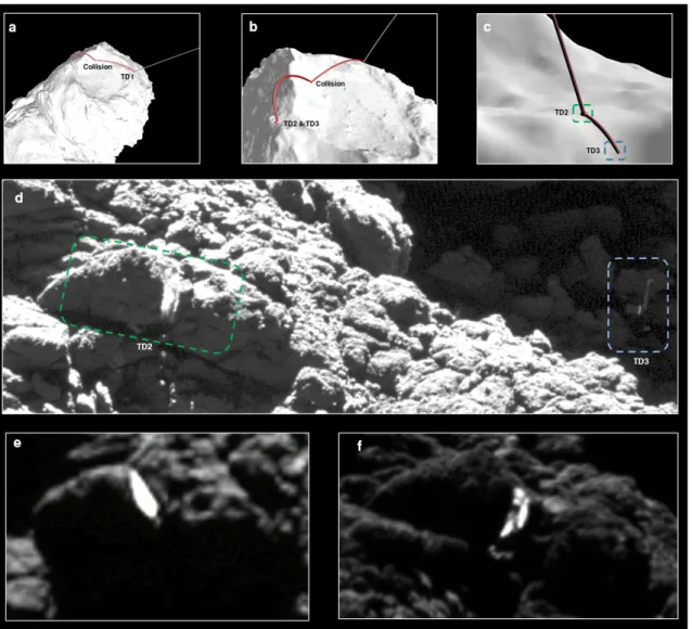
Fig. 1 – Philae landing trajectory, TD2 and Philae, Visible ice. Images a, b and c : three views showing the Philae landing trajectory as it crosses the surface of the comet (shape model) highlighting the locations of Touchdown 1 (TD1), Collision, Touchdown 2 (TD2) and Touchdown 3 (TD3). OSIRIS image d (2nd Sept 2016 19:59 UT; 0.049 m/pixel) is overexposed in order to show the skull-top crevice and the Philae lander hidden in the distant shadows. Images e and f show views of the ice in the crevice (6th
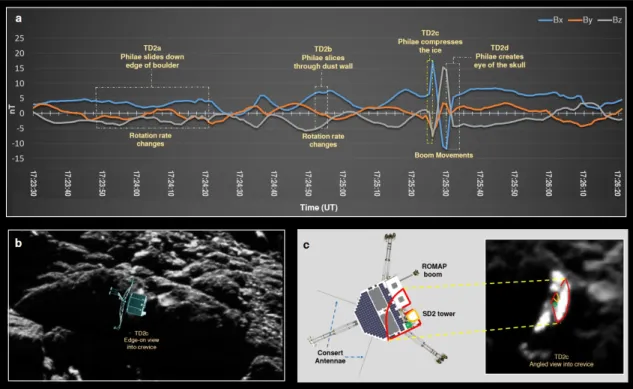
Fig. 2 A ROMAP guide and Philae impacts TD2c : Panel a shows the ROMAP magnetometer rotation/boom measurements matching Philae touchdown events versus time (see Methods and Supplementary Methods). OSIRIS Image b focusses on TD2c where the lander compressed the ice in the crevice (2nd September 2016). Image c shows
an overhead view of the Philae lander highlighting its instruments. The red, orange and green markings map to the impression in the ice (OSIRIS image 24th August 2016). See
Supplementary Video 2 showing a fly-over of the crevice and Supplementary Video 3 for an animation of this current figure.
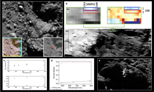
Fig. 3 Multi-instrument view of the water ice. a OSIRIS inset-images (left : multi-filter view, right : star and black dot position for plots c,d) within NAC image (14th June 2014
10:29UT). b 0.55 µm VIRTIS-M Hyperspectral cube (V1_00424522185.QUB) of the Abydos region (14° June 2016 10:51-11:35 UT) with skull-top ridge located in the green box. The inset panels zoom on spectral slope (left) and I/F image (right). c plot of reflectance and I/F versus wavelength and d the measured albedo. OSIRIS Image e (2nd Sept 2016) shows the crevice edge-on with e1 (crevice width) 1.03 ± 0.07 m and e2 (compression width) 0.246 ± 0.049m.
Extended Data Fig. 1 Pre & post-landing image comparison. This figure compares the skull-top ridge location (yellow rectangle) as it looked in OSIRIS image a for pre-landing (22nd October 2014) and image b for post-landing (14th May 2016). The yellow
dashed lines outline the skull-top boulders (see Supplementary Video 3 for a detailed comparison) while context terrain similarities between images are shown in blue dashed lines.. Although the spacecraft distance is the same (approx. 8km), the sun illumination and Rosetta viewing geometry differ between the images. An arrow points at the Philae lander location in the post-landing image.
Extended Data Fig. 2 OSIRIS Colour composites of skull-top boulders Images a & b Pre-landing images of “skull-top” boulders (inset); RGB setting: “green”= F24 (480.7 nm), “red”= F22 (649.2 nm), “blue”= F16 (360.0 nm). Images c-e “skull-top” boulders observed December 2014; RGB setting: “green”= “red”= F22 (649.2 nm), “blue”= F24 (480.7 nm). Images f-i The “skull-top” boulders observed in March 2016; RGB setting: “green”= “red”= F22 (649.2 nm), “blue”= F24 (480.7 nm).. Images j-m Color composite of the “skull-top” boulders in early and mid-June 2016; RGB setting: “green”= F24 (480.7 nm), “red”= F22 (649.2 nm), “blue”= F16 (360.0 nm).
Extended Data Fig. 3 Skull-top crevice illumination geometry. a Transparent overlay of the azimuth plots from the insets on a 12th June 2016 OSIRIS NAC image. The red
highlight is the sun illumination from Philae landing to end of mission. Each concentric circle represents 30 degrees azimuth. The green line maps the edge of the sun illumination. The yellow line shows the crevice horizon mask. b 21st August 19:19-19:24
azimuth plot with red-lined horizon mask of skull-top crevice. Inset OSIRIS image from that date/time shows crevice is illuminated. Red dot is sun angle and green dot is Rosetta viewing angle
Extended Data Fig. 4 VIRTIS water ice analysis plots – Average I/F of skull-top boulder location (blue curve) and on the nearby dark terrain (red curve) before (plot a) and after (plot b) normalization at 550 nm. Plot c : theoretical abundance of water ice as a function of the spectral slope in the visible spectral channel43. Black dots and dashed lines indicate a water ice rich region observed by VIRTIS
to calibrate the theoretical curves. The x-axis values correspond to slope values scaled to the dark terrain unit viewing conditions (Fig 3b. panel b1 red box) for observation V1_00424522185.QUB.
Extended Data Fig. 5 Combined ROMAP and RPC-MAG magnetic field and boom
measurements. The three components of the magnetic field observations are shown starting before TD2 at 17:23:00 UTC and ending shortly after the boom movement was detected. This figure also shows the concurrent orbiter RPC-MAG observations as reference. See Methods and
Extended Data Fig. 6 : Philae Interaction geometry and Boulder volume-filling factor. a Interaction geometry of Philae with the ice/dust at moment of deepest penetration in TD2c. b Philae superimposed on OSIRIS image (2nd September 2016)
showing equivalent interaction geometry as in a. c Compressive stress curves for a hierarchical makeup. Note the volume-filling factor Φ denotes packing of porous pebbles only; these are then further packed to make up the whole boulder. See Methods for detailed explanation.
Extended Data Table 1 - Estimation of the water ice content of the bright spot observed at the crevice of the “skull” boulder on three separate observations by the OSIRIS instrument in mid June 2016. ∆: distance between the spacecraft and the comet surface, α: phase angle and ρ: water ice fraction. The 14th June 2016 10:30:32 image
provides the highest value as the illumination into the crevice and viewing condition was the best of the three opportunities.
Extended Data Table 2 Philae lander dynamics through TD2a to TD2d Summary of the underlying values and results for TD2, including timing, as described in the Methods (Philae Lander Dynamics at Touchdown 2c point only) and Supplementary Methods (see section on “Detailed Description of flight through TD2 from ROMAP/RPC-MAG Analysis”). Supplementary Video 4 provides an animation showing the dust wall referred to in the table.