The use of hydrological and geoelectrical data to fix the boundary conditions of a ground water flow model: a case study

(1)

HAL Id: hal-00305218

https://hal.archives-ouvertes.fr/hal-00305218

Submitted on 1 Jan 2003

HAL is a multi-disciplinary open access archive for the deposit and dissemination of sci-entific research documents, whether they are pub-lished or not. The documents may come from teaching and research institutions in France or abroad, or from public or private research centers.

L’archive ouverte pluridisciplinaire HAL, est destinée au dépôt et à la diffusion de documents scientifiques de niveau recherche, publiés ou non, émanant des établissements d’enseignement et de recherche français ou étrangers, des laboratoires publics ou privés.

The use of hydrological and geoelectrical data to fix the

boundary conditions of a ground water flow model: a

case study

M. Giudici, M. Manera, E. Romano

To cite this version:

M. Giudici, M. Manera, E. Romano. The use of hydrological and geoelectrical data to fix the bound-ary conditions of a ground water flow model: a case study. Hydrology and Earth System Sciences Discussions, European Geosciences Union, 2003, 7 (3), pp.297-303. �hal-00305218�

(2)

The use of hydrological and geoelectrical data to fix the boundary conditions of a ground water flow model: a case study Hydrology and Earth System Sciences, 7(3), 297303 (2003) © EGU

The use of hydrological and geoelectrical data to fix the boundary

conditions of a ground water flow model: a case study

Mauro Giudici, Martina Manera and Emanuele Romano

Università degli Studi di Milano, Dipartimento di Scienze della Terra, Sezione di Geofisica, Via Cicognara 7, I-20129 Milano, Italy Email for corresponding author: Mauro.Giudici@unimi.it

Abstract

To assess whether the hydrometric level of an artificial lake in a quarry near Milan (Italy) could be assigned as a Dirichlet boundary condition for the phreatic aquifer in a fine scale groundwater flow model, hydrological measurements of piezometric head and rainfall rate time series have been analysed by spectral and statistical methods. The piezometric head close to the quarry lake proved to be well correlated with seasonal variations in the rainfall. Furthermore, geoelectrical tomography detected no semi-permeable layer between the phreatic aquifer and the lake, so the contact between surface and ground water is good. Finally, a time-varying prescribed head condition can be applied for ground water flow modelling.

Keywords: ground water flow, boundary conditions, surface and ground water interactions, geoelectrical tomography, statistical analysis.

Introduction

The application of a groundwater flow model requires the assignment of the boundary conditions, not always available for fine scale models of small areas because the physical borders of the aquifer system may be far from the modelled area (Mehel and Hill, 2002; Romano et al., 2002). In particular, when the boundary conditions are represented by the flow across a border (Neumann boundary conditions), a potential must be assigned at a point in the domain (Dirichlets datum) to obtain a unique solution.

In the development of a fine scale model (modLambro) for the part of the aquifer system of Milan beneath the Lambro Park (Romano et al., 2002), the boundary conditions were obtained from a coarser scale model (ModMil) for the ground water flow over the whole city area (Giudici et al., 2000). At the south-eastern corner of the domain modelled with modLambro are some small artificial lakes whose water levels could be assigned as the Dirichlets datum provided that the hydraulic contact between the lake and the phreatic aquifer ensures equilibrium between the water level in the lake and the head in the aquifer.

Hence, the conditions at one of these small artificial lakes has been studied. Since in the modelled area the water table is more than 10 m below ground level and the lake is up to

35 m deep, the aquifer and the lake can exchange water; the problem is whether the heads of water in the lake and the aquifer are equal or whether water exchange occurs through less permeable materials between the lake and the aquifer. In the absence of hydrometric measurements, information on the characteristics of the hydraulic contact between the lake and the aquifer has been explored using geoelectrical prospecting; the possibility of assigning a constant or time-varying potential by analysing piezometric head and rainfall rate data has been evaluated. The time series of water table oscillations has been analysed statistically: the phreatic head has been correlated with the cumulative rainfall for different time intervals prior to the piezometric measurements.

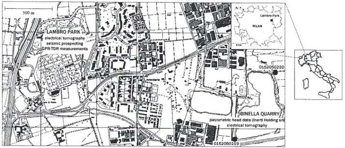
The area investigated is near the Binella quarry, a facility to dig sand and gravel in the municipality of Segrate, a suburb of Milan. The site is largely uncovered and characterised by an artificial quarry lake, about 0.25 km2_in

area (Fig. 1).

The domain studied is part of the Po river alluvial plain and the sediments investigated, deposited in glacial and fluvio-glacial environments since the middle Pleistocene, consist mainly of sandy-gravel layers, separated by silt and clay lenses; a continuous layer of fine grain material, some 30 m below ground level, separates the shallow phreatic

(3)

Mauro Giudici, Martina Manera and Emanuele Romano

aquifer and semi-confined aquifers, which together form the so called traditional aquifer, i.e. the aquifer most exploited for water abstraction.

The investigation benefited from other field data and modelling results obtained by geophysical prospecting nearby (seismic, geoelectrical, GPR and TDR). These helped to clarify the information on the hydrogeological structure and the physical properties under the Lambro Park.

Hydrological and geophysical data

To the geoelectrical measurements made in this study have been added rainfall rate data received from the Istituto di Fisica Generale Applicata of the University of Milan as well as piezometric head data from Inerti Holding srl, the company managing the Binella quarry.

HYDROLOGICAL DATA

Piezometric heads are measured monthly at two piezometers close to the shore of the Binella quarry lake (Fig. 1.). Data from March 1998 to October 2002 have been analysed, along with piezometer readings close to other quarries managed by the same company some kilometres away.

The linear correlation coefficient between the piezometric heads for the two piezometers is 0.99 so it is very likely that the two temporal series are linearly dependent.

Hourly meteorological data are available from January 1999 to December 2002.

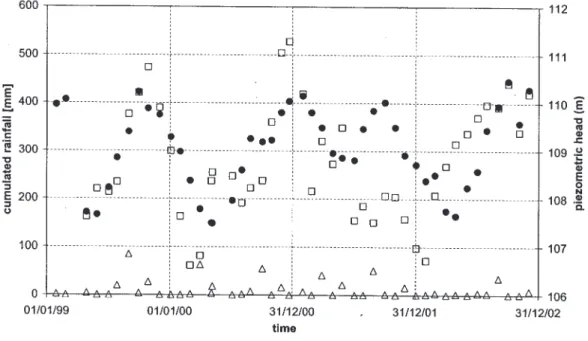
In Fig. 2 the phreatic head at piezometer 0152050219 is

plotted against time, together with two series that correspond to the rainfall accumulated over short and long time intervals before the measurement of the piezometric head. In particular, a short interval of five days and a long interval of 90 days have been assessed. The plot shows that the available head data are correlated with the precipitation accumulated over the longer time intervals but not over the shorter time period.

GEOPHYSICAL DATA

The geoelectrical data were obtained with the 16G computer-controlled automatic acquisition system made by P.A.S.I. srl, equipped with 16 electrodes, using a dipole-dipole array. Four linear arrays were run parallel to the south shore of the quarry lake, about 100 m east of piezometer 0152050219. For the first array, the electrodes were arranged on the ground with an electrode spacing of 5 m and a total

Fig. 1. Map of the study area. The Binella quarry is located at the South-East corner, the dots with

the code show the positions of the wells. The area of the Lambro park, where further geophysical data have been acquired, is shown. (The topographic base is the CTR 1:10000, realised by Regione Lombardia)

Fig. 3. Geometry of the four surveys performed along the south

(4)

The use of hydrological and geoelectrical data to fix the boundary conditions of a ground water flow model: a case study

Fig. 2. Diagram of the time series of piezometric head (circles) and cumulated rainfall for different time

intervals (triangles and squares correspond to time intervals of 5 and 90 days, respectively).

length of 75 m. To explore the shallowest part of the underground better, three arrays with the spacing between adjacent electrodes reduced to 2 m were used; these arrays were partially overlapped, to cover approximately the same area of the first array (Fig. 3).

Data processing and results

SPECTRAL AND STATISTICAL ANALYSIS OF HYDROLOGICAL DATA

The water table oscillations were studied by spectral analysis of piezometric head time series; the power spectrum shows two dominant periods of six and 12 months. Both the Fourier analysis and the autocorrelation function of the precipitation series, converted to a monthly series, show a dominant period of six months.

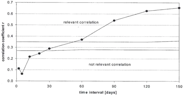
The relationship between the water table level and the rainfall rate has been studied statistically. Because it is unlikely that the head data are strongly correlated with the precipitation immediately before the head measurements (Fig. 2), precipitation was accumulated over time intervals of 2150 days prior to the head measurements. The linear correlation coefficient, r, between the phreatic head and the rainfall thus calculated has been used in evaluating the link between the two series. Figure 4 shows r as a function of the time interval for piezometer 0152050219; the maximum value of r is 0.69, corresponding to the longest time interval (150 days, i.e. five months).

The linear correlation coefficient should be close to 1 to have a relevant correlation. In order to quantify this, the probability that the absolute value of the linear correlation coefficient be greater than a given value even if the piezometric data were not linearly correlated with the cumulated rainfall (null hypothesis) has been estimated. Two probability ranges have been considered:

not relevant correlation, when the probability of the null hypothesis exceeds 5%;

relevant correlation, when the probability of the null hypothesis is smaller than 1%.

Following standard estimates (Taylor, 1997), the correlation has appeared to be not relevant for time intervals shorter than 21 days and relevant for time intervals longer than 60 days.

GEOELECTRICAL DATA PROCESSING AND INTERPRETATION

Geoelectrical data were processed and inverted using computer codes Res2Dinv and Res3Dmod (Loke, 2003). Res2Dinv identifies a two-dimensional subsurface resistivity distribution the response of which fits the measured apparent resistivity pseudo-section. Res2Dinv calculates the apparent resistivity corresponding to a given subsurface resistivity distribution, using a finite difference approximation to compute the electrical field (Dey and Morrison, 1979a; Loke, 1994); the program identifies the optimal resistivity

(5)

Fig. 4. Linear correlation coefficient trend between the piezometric head of well 0152050219 and the cumulated

rainfall in a progressive sequence of time. Areas in different greys correspond to the linear correlation range between the two variables (Taylor, 1997).

which minimises the RMS of the differences between modelled and observed apparent resistivity in an iterative procedure. Res3Dmod implements a 3-D finite difference model (Dey and Morrison, 1979b) to compute the apparent resistivity corresponding to a given spatial distribution of electrical resistivity.

The use of a 3-D inversion was not justified by the geometry of the data collection. Instead, a method was developed to reduce the effect of topography outside the survey line on the measured values of apparent resistivity. The arrays run parallel to the shore, over a small terrace, the top of which is about 6 m above the water level in the quarry lake. Res3Dmod has been used to estimate the distortion effect of the terrace slope and of the water basin on the geoelectrical measurements. Figure 5, a vertical section perpendicular to the shore, represents the geometry of the field data acquisition and of the discrete model. The values of resistivity have been assigned on the basis of the geoelectrical stratigraphy obtained from a preliminary inversion of the geoelectrical data. The terrace slope has been modelled as a vertical contact, 6m thick, between the air and the ground. The lake is represented as a conductive body with a rectangular area of coordinates 16 < x < 4 m, 6 < z < 15 m and ρ = 40 Ωm. Two forward models have been developed for arrays with spacings of 2 and 5 m along the y-direction and for total lengths of 75 and 30 m respectively, to simulate the distribution of the apparent resistivity for both field acquisitions.

Apparent resistivity pseudosections have been computed,

corresponding to spacings of 2 and 5 m between the electrodes and located 2 and 14 m from the edge of the terrace. The apparent resistivity for the pseudosections near the edge, which is roughly the position of the arrays used in the acquisition of real data, is represented by ρn, whereas the apparent resistivity for the arrays far from the edge is denoted by ρf. The latter arrays are far enough from the edge of the terrace to avoid the effects of topographic anomalies, while the former arrays, near the edge, are influenced by the resistive medium, the air and the lake.

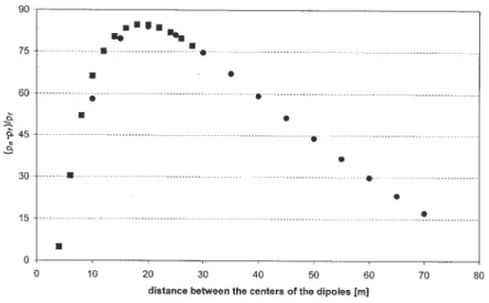
The differences between the two pseudosections have been quantified as a percentage of ρf. and represented in Fig. 6, where (ρn ρf.) / ρf. is plotted as function of the distance between the centres of the potentiometric and the current dipoles, for spacings of both 2 and 5 m. The differences between ρn and ρf. are estimated between 50% and 83% for distances between 7 and 45 m. If the distance is less than 6 m or greater than 60 m, the discrepancy between the two apparent resistivity sections is always less than 40%. This shows that the topographic effect has altered the values of the collected geoelectrical data and, in particular, the resistivity values have been overestimated. Finally, the results of Fig. 6 have been used to correct the measured apparent resistivity with the application of an adjustment factor, ρcorrected.= ρmeasured ρf./ ρn.

The corrected tomographic data have then been inverted with Res2Dinv. To exploit the information given by all the arrays simultaneously, all the measured data were edited into a single file containing both the measurements for the

(6)

array with 5 m spacing greater exploration depth and with 2 m spacing better resolution. The total number of measurements of the four arrays is 358. Several tests have been performed with this data set to evaluate the effects of different alternatives as follows:

1. monitoring and treating noisy data;

2. changing the discretisation grid for the finite difference forward modelling to compute the modelled apparent resistivity pseudo-section;

3. reducing the weights of the side block on the calculation of the Jacobian matrix used for the iterative inverse procedure;

4. selecting different inversion methods.

The main characteristics of the final processing and inversion procedure are summarised in the following paragraphs.

The discrete grid has been subdivided into 999 blocks of horizontal width 1 m and layer thickness increasing by 110% with depth.

Since the data set contains a small number of noisy measurements, the robust inversion option has been selected. This L1 norm inverison method (Farquharson and Oldenburg, 1998; Loke et al., 2001) constrains the inversion routine through a cut-off factor, which greatly reduces the

Fig. 5. Three-dimensional resistivity model section along x, z.

Fig. 6. Diagram of

(

ρn−ρf

)

ρf for dipole-dipole arrays with spacing of 2 and 5 m, as a function of the distance between the centres of the dipoles. Squares and circles correspond to spacing of 2 and 5 m, respectively.

(7)

effect of data points where the differences between the measured and computed apparent resistivity values are greater than 5%.

The results of the inversion of the geoelectrical data, corrected by the topographic anomalies, are shown in Fig. 7. Three geoelectrical layers can be identified (Fig. 7-c): (1) a shallow geoelectrical layer with a thickness of about 2 m and a resistivity range between 200 and 1000 Ω⋅m, with the highest values in the region between 12 and 32 m from the beginning of the acquisition line; (2) an intermediate geoelectrical layer with a thickness of about 4.5 m and a resistivity range between 700 and 1500 Ω⋅m, with some isolated resistive anomalies; and (3) a geoelectrical layer with resistivity less than 300 Ω⋅m.

To build a lithological scheme of the study area, the inversion model results have been compared with the well stratigraphy and with the piezometric head, sampled near the Binella quarry. The discontinuity between the geoelectrical layers (2) and (3) coincides not with a lithological discontinuity in the sandy-gravel ground but the saturated-unsaturated limit (Fig. 8).

The geoelectrical results at the Binella quarry have been compared with the results obtained at the Lambro Park area; they are quite similar for the geoelectrical layers (2) and (3)

Fig. 7. Robust data constrain inversion: (a) measured pseduosection of apparent resistivity; (b) calculated

pseudosection of apparent resistivity; (c) resistivity distribution obtained from the inversion.

and small discrepancies are probably due to heterogeneities in the quantities of sand, gravel and water content whereas, in the Lambro Park area, a shallow fine-grained soil is present with a resistivity of about 100 Ω⋅m.

Fig. 8. Correlation between the stratigraphy of well 0152050019

(8)

Conclusions and perspectives

The temporal trend of the hydrometric level of the Binella quarry lake can be evaluated by combining statistical analysis with hydrological considerations. The correlation coefficients show that the piezometric head sampled approximately monthly correlates with the rainfall accumulated over a prior time interval longer than 90 days but not with rainfall collected over a period of less than 30 days. This effect can be understood by considering the interaction between the lake and the aquifer. After a rain event, the rise in the water table should be greater than that in the lake by a factor, which depends on the effective porosity. However, the rise in the water table is slowed by the infiltration through the unsaturated zone, more than 10 m thick in this area; the velocity of water in the unsaturated zone depends not only on the physical properties of the soil, but also on the soil water content before the rainfall, on the rain intensity and duration. The exchange from the aquifer to the lake and vice versa is therefore quite complex and varies with time. Hence, the lake acts as a compensation basin, with a slow response time, which influences the temporal piezometric variations near the lake itself.

Since monthly sampling of the phreatic level does not allow investigation of the effect of a single rain event on the piezometric head, one can only hypothesise a direct dependence between the water table oscillation and the hydrometric level for a seasonal time interval.

Geoelectrical data have shown a discontinuity of resistivity at a depth of about 6 m, which correlates well with the water table and with the lake level. The geoelectrical survey has not revealed the presence of sediments with small permeability, which could hinder the water exchange between the aquifer and the lake. Therefore it is possible to suppose that the lake and the phreatic aquifer have a good hydraulic contact, so that the hydrometric level of the Binella quarry can be used as Dirichlet datum in modLambro, even if time-varying and related to the seasonal rainfall.

The time series of piezometric head at another two quarries, located at a distance of 5 km east and 10 km southeast from the Binella quarry have also been considered. The correlation coefficients between the piezometric head for those quarries with the cumulated rainfall are greater than for the Binella quarry. This could be an effect of the differences between mining activity and lake fluctuations at the three sites.

This work opens perspectives for future developments: the temporal lake trend could be analysed better by taking direct measurements of the hydrometric level and developing a mathematical model which simulates the hydrometric head trend as a function of the recharge and of

the ground-surface water flow. Furthermore, the simultaneous use of geophysical (geoelectrical tomography) and hydrological (rainfall and piezometric head) data can be extended to other artificial lakes present in the modLambro domain.

Acknowledgements

M. Maugeri and L. Buffoni (Istituto di Fisica Generale Applicata, Università degli Studi di Milano) are thanked for the rainfall rate data, M. Noris and M. Carini (Inerti Holding s.r.l.) for the piezometric head data, C. Arduini and F. Di Palma (Provincia di Milano) for the lithological well logs and Inerti Holding s.r.l. for permission to make the geolectrical survey. Finally, Professor Gianni Ponzini is thanked for discussions.

The work has been supported by the research programme The contribution of geophysics to hydrogeological risk assessment: exploration, monitoring and modelling, coordinated by Professor Mauro Giudici and financed in part by the Italian Ministry for Instruction, University and Research.

References

Dey, A. and Morrison, F., 1979a. Resistivity modeling for arbitrarily shaped two-dimensional structures. Geophys. Prospect., 27, 10201036.

Dey, A. and Morrison, F., 1979b. Resistivity modeling for arbitrarily shaped three-dimensional structures. Geophysics, 44, 753780.

Farquharson, C.G. and Oldenburg, D.W., 1998. Non-linear inversion using general measures of data misfit and model structure. Geophys. J. Int., 134, 213227.

Giudici, M., Foglia, L., Parravicini, G., Ponzini, G. and Sincich, B., 2000. A quasi three dimensional model of water flow in the subsurface of Milano (Italy): the stationary flow. Hydrol. Earth Syst. Sci., 4, 113124.

Loke, M.H., 1994. The inversion of two-dimensional resistivity data. PhD thesis, University of Birmingham, UK.

Loke, M.H., 2003. Tutorial: 2-D and 3-D electrical imaging surveys. Geotomo Software, Penang, Malaysia.

Loke, M.H., Acworth, I. and Dahlin, T., 2001. a comparison of smooth and blocky inversion methods in 2D electrical imaging surveys. Proc. ASEG 15th Geophysical Conference, Brisbane, Australia.

Mehel, S. and Hill, M.C., 2002. Development and evaluation of a local grid refinement method for block centred finite difference groundwater models using shared nodes. Advan. Water Resour.,

25, 497511.

Romano, E., Giudici, M. and Ponzini, G., 2002. Simulation of interactions between well fields with nested models: a case study, Acta Univ. Carolinae Geologica, 46, 637640.

Taylor, J.R., 1997. An introduction to error analysis: the study of uncertainties in physical measurements. University Science Books, Sausalito, CA, USA.