Whistler wave occurrence and the interaction with strahl electrons during the first encounter of Parker Solar Probe

HAL Id: hal-03265977

https://hal.sorbonne-universite.fr/hal-03265977

Submitted on 21 Jun 2021

HAL is a multi-disciplinary open access

archive for the deposit and dissemination of

sci-entific research documents, whether they are

pub-lished or not. The documents may come from

teaching and research institutions in France or

abroad, or from public or private research centers.

L’archive ouverte pluridisciplinaire HAL, est

destinée au dépôt et à la diffusion de documents

scientifiques de niveau recherche, publiés ou non,

émanant des établissements d’enseignement et de

recherche français ou étrangers, des laboratoires

publics ou privés.

strahl electrons during the first encounter of Parker

Solar Probe

V. Jagarlamudi, T. Dudok de Wit, C. Froment, V. Krasnoselskikh, A. Larosa,

L. Bercic, O. Agapitov, J. Halekas, M. Kretzschmar, D. Malaspina, et al.

To cite this version:

V. Jagarlamudi, T. Dudok de Wit, C. Froment, V. Krasnoselskikh, A. Larosa, et al.. Whistler wave

oc-currence and the interaction with strahl electrons during the first encounter of Parker Solar Probe.

As-tronomy and Astrophysics - A&A, EDP Sciences, 2021, 650, pp.A9. �10.1051/0004-6361/202039808�.

�hal-03265977�

Astronomy

_&

Astrophysics

Special issue

A&A 650, A9 (2021) https://doi.org/10.1051/0004-6361/202039808 © V. K. Jagarlamudi et al. 2021

Parker Solar Probe: Ushering a new frontier in space exploration

Whistler wave occurrence and the interaction with strahl

electrons during the first encounter of Parker Solar Probe

V. K. Jagarlamudi

1,2

_{, T. Dudok de Wit}

1

_{, C. Froment}

1

_{, V. Krasnoselskikh}

1

_{, A. Larosa}

1

_{, L. Bercic}

3,4

_{, O. Agapitov}

5

_,

J. S. Halekas

6

_{, M. Kretzschmar}

1

_{, D. Malaspina}

7,8

_{, M. Moncuquet}

3

_{, S. D. Bale}

5,9,10,11

_{, A. W. Case}

12

_,

J. C. Kasper

12,13,14

_{, K. E. Korreck}

12

_{, D. E. Larson}

5

_{, M. Pulupa}

5

_{, M. L. Stevens}

12

_{, and P. Whittlesey}

5

1_{LPC2E/CNRS, 3 avenue de la Recherche Scientifique, 45071 Orléans Cedex 2, France}

2_{National Institute for Astrophysics-Institute for Space Astrophysics and Planetology, Via del Fosso del Cavaliere 100, 00133 Roma,}

Italy

e-mail: vamsee.jagarlamudi@inaf.it

3_{LESIA, Observatoire de Paris, Université PSL, CNRS, Sorbonne Université, Université de Paris, 5 place Jules Janssen,}

92195 Meudon, France

4_{Physics and Astronomy Department, University of Florence, Via Giovanni Sansone 1, 50019 Sesto Fiorentino, Italy} 5_{Space Sciences Laboratory, University of California, Berkeley, CA 94720-7450, USA}

6_{Department of Physics and Astronomy, University of Iowa, Iowa City, IA 52242, USA}

7_{Laboratory for Atmospheric and Space Physics, University of Colorado, Boulder, CO 80303, USA} 8_{Astrophysical and Planetary Sciences Department, University of Colorado, Boulder, CO 80303, USA} 9_{Physics Department, University of California, Berkeley, CA 94720-7300, USA}

10_{The Blackett Laboratory, Imperial College London, London, SW7 2AZ, UK}

11_{School of Physics and Astronomy, Queen Mary University of London, London E1 4NS, UK} 12_{Smithsonian Astrophysical Observatory, Cambridge, MA, 02138, USA}

13_{Climate and Space Sciences and Engineering, University of Michigan, Ann Arbor, MI 48109, USA} 14_{BWX Technologies, Inc., Washington, DC 20002, USA}

Received 30 October 2020 / Accepted 12 January 2021

ABSTRACT

Aims. We studied the properties and occurrence of narrowband whistler waves and their interaction with strahl electrons observed

between 0.17 and 0.26 au during the first encounter of Parker Solar Probe.

Methods. We used Digital Fields Board band-pass filtered (BPF) data from FIELDS to detect the signatures of whistler waves.

Additionally parameters derived from the particle distribution functions measured by the Solar Wind Electrons Alphas and Protons (SWEAP) instrument suite were used to investigate the plasma properties, and FIELDS suite measurements were used to investigate the electromagnetic (EM) fields properties corresponding to the observed whistler signatures.

Results. We observe that the occurrence of whistler waves is low, nearly ∼1.5% and less than 0.5% in the analyzed peak and

aver-age BPF data, respectively. Whistlers occur highly intermittently and 80% of the whistlers appear continuously for less than 3 s. The spacecraft frequencies of the analyzed waves are less than 0.2 electron cyclotron frequency ( fce). The occurrence rate of whistler waves

was found to be anticorrelated with the solar wind bulk velocity. The study of the duration of the whistler intervals revealed an anticor-relation between the duration and the solar wind velocity, as well as between the duration and the normalized amplitude of magnetic field variations. The pitch-angle widths (PAWs) of the field-aligned electron population referred to as the strahl are broader by at least 12 degrees during the presence of large amplitude narrowband whistler waves. This observation points toward an EM wave electron interaction, resulting in pitch-angle scattering. PAWs of strahl electrons corresponding to the short duration whistlers are higher com-pared to the long duration whistlers, indicating short duration whistlers scatter the strahl electrons better than the long duration ones. Parallel cuts through the strahl electron velocity distribution function (VDF) observed during the whistler intervals appear to depart from the Maxwellian shape typically found in the near-Sun strahl VDFs. The relative decrease in the parallel electron temperature and the increase in PAW for the electrons in the strahl energy range suggests that the interaction with whistler waves results in a transfer of electron momentum from the parallel to the perpendicular direction.

Key words. waves – scattering – plasmas – Sun: heliosphere – magnetic fields

1. Introduction

Whistler waves are right-handed polarized electromagnetic modes observed between the lower hybrid frequency ( fLH) and

electron cyclotron frequency ( fce) in the plasma frame. The

range between fLHand fce is usually referred to as the whistler

range since whistler waves are the dominant electromagnetic modes observed in this range. In the solar wind, whistlers are

dominantly observed in the range between fLHand 0.5 fce(Zhang

et al. 1998;Lacombe et al. 2014;Tong et al. 2019a;Jagarlamudi et al. 2020).

Whistler wave modes through their interaction with electrons are thought to be one of the prime contributors in the regula-tion of fundamental processes in the solar wind (Vocks & Mann 2003; Pagel et al. 2007;Kajdiˇc et al. 2016; Tang et al. 2020). Wave particle interactions, such as those between whistler waves

A9, page 1 of10

Open Access article,published by EDP Sciences, under the terms of the Creative Commons Attribution License (https://creativecommons.org/licenses/by/4.0),

and electrons, might play a significant role in explaining many physical process such as the heating, acceleration, and scattering of the particles in the solar wind. The electron velocity dis-tribution can be mainly divided into three parts: a low energy isotropic distribution called the core, a high energy isotropic part called the halo, and the heliospheric magnetic field aligned high energy component called the strahl (Feldman et al. 1978;Pilipp

et al. 1987a,b). While collisions were shown to isotropise the

dense low energy electron population referred to as the electron core, they are not sufficient to regulate the more tenuous higher energy electron populations such as the halo and strahl (Ogilvie & Scudder 1978;Pilipp et al. 1987a). Wave particle interactions have a crucial role in explaining the phenomena happening in the high energy ranges.

Due to their small mass, electrons reach high thermal veloc-ities in the hot solar corona. The fastest electrons such as strahl can escape the solar corona almost undisturbed, carrying the majority of the heat flux stored in the solar wind. The rate of radial decrease in electron heat flux from the Sun suggests the existence of the scattering mechanism during solar wind expansion (Scime et al. 1994; Hammond et al. 1996; Štverák

et al. 2015). Therefore, understanding the evolution of strahl

electrons and the wave modes interacting with them gives us valuable insight into the global solar wind thermodynamics and energy transport. Observations have shown that the strahl pitch-angle width (PAW) increases as we move further from the Sun (Hammond et al. 1996;Graham et al. 2017;Berˇciˇc et al. 2019). It is also seen that the relative density of the electron halo increases, while the relative density of the strahl decreases as we move away from the Sun (Maksimovic et al. 2005;Štverák et al. 2009). Whistler waves with their interaction with strahl electrons could be able to explain the observed evolution of electron veloc-ity distributions (Vocks 2012; Kajdiˇc et al. 2016; Boldyrev & Horaites 2019;Tang et al. 2020).

There are quite a few studies on the whistler waves in the free solar wind at 1 au. One of the early studies to show the clear presence of whistler waves in the free solar wind was done by

Zhang et al.(1998). In their study, the authors used the

high-resolution electric and magnetic field wave form data on board the Geotail spacecraft. They observed that whistler waves have frequencies between 0.1 fceand 0.4 fce, and the wave vectors were

dominantly aligned to the magnetic field direction and propagat-ing in the anti-sunward direction. Whistler wave packets were observed for short durations (less than 1 s).

Lacombe et al. (2014), using the magnetic spectral matrix

routine measurements of the Cluster/STAFF instrument, stud-ied the long duration whistlers (5–10 min). They have studstud-ied 20 events, which were observed in the slow wind with a fre-quency range between 0.1 fce and 0.5 fce. The observed waves

were quasi-parallel and narrowband. Tong et al. (2019a) car-ried out a large statistical study of whistler waves using 3 yr of magnetic field spectral data from the ARTEMIS (Acceler-ation, Reconnection, Turbulence, and Electrodynamics of the Moon’s Interaction with the Sun) spacecraft. They show that the occurrence of whistler waves was dependent on the electron tem-perature anisotropy, and the amplitude of whistler waves were typically small, below 0.02 of the background magnetic field.

A statistical study on whistler waves in the solar wind in the inner heliosphere (0.3–1 au) was performed byJagarlamudi et al.(2020), who used the search coil spectral data to identify the signatures of whistler waves. Their observed whistler waves have frequencies between 0.05 fce and 0.3 fce. They show

differ-ent properties of whistler waves and find that the slower the bulk velocity of the solar wind, the higher the occurrence of whistlers.

They show that the occurrence probability of whistler waves is lower as we move closer to the Sun and suggest that whistler occurrence and variations in the halo and core anisotropy as well as the heat flux values were related.

Cattell et al. (2020) studied the large amplitude whistler

waves in the solar wind at frequencies of 0.2–0.4 fce using

the STEREO electric and magnetic field waveforms. These waves were often observed in association with the stream inter-action regions. Their studies show that the large amplitude and obliquely propagating, less coherent whistlers were able to resonantly interact with electrons over a broad energy range.

A recent study by Agapitov et al. (2020), using the Parker Solar Probe’s (PSP’s) magnetic and electric waveform data, has shown the presence of whistler waves when magnetic field dips were observed around switchback boundaries. The observed waves were quasi-parallel to dominantly oblique, wave normal angles were close to the resonance cone. The observed whistler wave packets have frequencies below 0.1 fce.

In this study, we focus on the whistler waves observed in the solar wind in the inner heliosphere between 0.17 and 0.26 au using the PSP’s first perihelion data. The PSP mission was launched in August 2018 to study the Sun closer than ever before through in situ measurements of solar wind (Fox et al. 2016).

We present the plasma properties (mainly the strahl electron properties) corresponding to the observed signatures of whistler waves identified using band-pass filtered (BPF) data. Studies by

Lacombe et al.(2014) at 1 au show that any local enhancement

(concentration of spectral power) observed in the magnetic field power spectral density in the frequency range of fLH and 0.5 fce

always corresponded to a narrowband whistler wave. For our study we assume that any local enhancement of spectral power observed in the frequency range between fLH and 0.5 fce is a

whistler wave signature (Zhang et al. 1998;Lacombe et al. 2014;

Jagarlamudi et al. 2020). The advantage of using band-pass data

is that we have high resolution continuous measurements, which allows us to analyze wave parameters statistically. However, the drawback is that we only have a single component of data avail-able and we do not have the polarization information, which has been compensated for by using the polarization information from the analysis of low time resolution cross-spectral data measured by the search coil magnetometer. Waveform data are useful to show the presence of whistlers in PSP’s data. However, only low frequency whistlers can be seen in the continuous waveform (with the sampling rate of 293 s−1_{and less), that is to say we can}

use waveforms for special cases, such as when there are drops in the magnetic field (Agapitov et al. 2020).

This article is structured as follows. In Sect.2we show the data and the methodology followed to identify the whistlers. In Sect. 3 we present the basic properties of whistler waves, as well as their occurrence and generation conditions. In Sect.4, using the strahl distributions, strahl PAW of electrons and the strahl parallel temperatures, we investigate the interaction between whistlers and strahl electrons. In Sect.5we present the conclusions for our study.

2. Methods and data for the whistler waves analysis

For the purposes of this paper, whistler analysis was performed using the data from the FIELDS (Bale et al. 2016) and SWEAP

(Kasper et al. 2016) instruments on board PSP during the first

encounter with the Sun (October 31–November 11, 2018). For the detection of the signatures of narrowband whistlers, we used the DC BPF measurements obtained from the Digital Fields Board (DFB) for FIELDS on board PSP (Malaspina et al. 2016). DFB

V. K. Jagarlamudi et al.: Whistler wave occurrence and the interaction with strahl electrons 102 103

Frequency (Hz)

f

LH

0.5f

ce 2.1 1.8 1.5 1.2 0.9 0.6 0.3 0.0 0.3 0.6

log(Peak BPF (nT))

02:13:33 02:14:03 02:14:33 02:15:03 02:15:33 02:16:03

3 Nov 2018

102 103

Frequency (Hz)

f

LH

0.5f

ce 2.0 1.8 1.6 1.4 1.2 1.0 0.8 0.6 0.4 0.2

log(Mean BPF (nT))

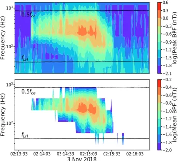
Fig. 1.Example of the peak and average band-pass filtered (BPF) data

used for the analysis of whistler waves.

gives the peak absolute and the average absolute values in each band-pass time series sample of ∼0.87 s, covering the frequency range of 0.5 Hz–9 kHz. The DC BPF data are organized in 15 frequency bins; for each, we have the mean amplitude of the magnetic field and the peak amplitude. BPF data are available for only one component of the magnetic field. Here, we have the Bu component of the SCM (Jannet et al. 2021). However, the main advantage compared to the three component cross-spectral data (∼28 s) is that BPF data are of a higher time resolution (∼0.87 s) and importantly both the peak and average data are available.

In Fig.1we show an example of peak and average BPF data using a 3 min interval when the BPF spectra showed a local enhancement of power. The data output of average BPF data is zero when the signal is very low in the corresponding frequency channels.

For the detection of the whistler signatures, we used a sim-ilar method as those used in the studies of Jagarlamudi et al.

(2020) andTong et al. (2019a), where a local enhancement of spectral power in the whistler range was inferred to indicate the presence of a narrowband whistler wave. First, we squared the peak and average BPF data and divided the squared values by the corresponding frequency bin width, which gives us an equiv-alent of the power spectral density (PSD) values. Using the PSD values, we identified the presence of one single local maximum in the whistler range which clearly stands out with respect to the PSD of the background turbulence (Alexandrova et al. 2012,

2020). Mathematically speaking, the indicator for whistler wave influenced PSD spectra is, as we go toward higher frequencies at a certain frequency, dPS D

d f will be positive and then it naturally

becomes negative again. However, we would like to mention that the suggested method could only be used with higher confidence for the average spectra. The reason is that the observations to date have shown the presence of whistlers in waveform data to the presence of local enhancement of spectral power in the average spectral data only.

An example of average PSD spectra which contain whistlers is shown in Fig.2, where spectra with distinctive local enhance-ment in the whistler range were selected. After selecting the spectra with whistler signatures, we studied the plasma

Fig. 2.Example of the spectra showing signatures of whistler waves in

the average BPF data as a function of f / fceon November 5, 2018. The

black vertical lines correspond to fLH/ fceand 0.5, respectively.

properties corresponding to those whistler signatures. We mainly focused on the strahl electron properties.

The advantage of BPF data is that thanks to their time res-olution of ∼0.87 s, they gives us a much better statistics and information on the duration of the whistlers compared to the low resolution spectral data (∼28 s). However, the cross-spectral data give us the approximate information on the absolute ellipticity. The study of cross-spectral data from PSP’s first perihelion byFroment et al.(2020) has shown that all the cross-spectra, which have shown the local enhancement of power in the whistler range, have higher ellipticity (∼1), indicating circu-lar pocircu-larization. This supports our assumption that spectra with local maxima in the BPF data in the whistler range are most probably due to the whistler waves.

To study the whistler wave properties, we used DC magnetic field data from the fluxgate magnetometer on board PSP (Bale

et al. 2016). We used electron and proton observations made by

the Solar Wind Electrons Alphas and Protons (SWEAP) exper-iment (Kasper et al. 2016). Proton densities and proton bulk velocities were obtained from their respective distribution func-tions measured by the Solar Probe Cup (SPC) at a cadence of ∼0.22 s (Case et al. 2020). The electron velocity distribution functions were measured by Solar Probe Analyzer (SPAN) elec-tron sensors on the ram (ahead) and anti-ram (behind) faces of the spacecraft (Whittlesey et al. 2020) and the data available for the first perihelion was of ∼28 s cadence.

We used the 4 Hz magnetic field data and interpolated these to the resolution of available BPF data. For proton and electron parameters, we considered the closest available value to the BPF interval with the whistler signature. The magnetic field data and the proton moments are taken from PSP Science Gateway1_.

The electron density, core temperatures, and heat flux are taken from the work of Halekas et al. (2020, 2021), where a bi-Maxwellian distribution is assumed to fit the core parame-ters. The strahl pitch-angle widths (PAWs), the cuts through the strahl electron VDFs, and the strahl parallel temperatures (Tsk)

are taken from the work ofBerˇciˇc et al.(2020). PAWs represent the full-width-at-half-maximum of a Gaussian fit to pitch-angle distribution functions at every instrument energy bin. The max-imal values of these fits by definition appear at a pitch-angle of 0 deg and thus form the parallel cut through the strahl VDF. In using this technique to study the properties of the strahl along the magnetic field, we account for the portion of the strahl VDF which is sometimes blocked by the spacecraft heat shield (see

Berˇciˇc et al. 2020for more details about the analysis). We note

1 _{https://sppgway.jhuapl.edu/}

that Tsk is a Maxwellian temperature of the strahl along the

magnetic field direction.

For our analysis, we also use the low-frequency receiver (LFR) data from the Radio Frequency Spectrometer on board PSP (Pulupa et al. 2017). Using the ∼7 s resolution LFR data, we detect the presence of Langmuir waves. The technique followed for the detection of Langmuir waves is similar to the whistler wave detection, that is to say usually the spectra influenced by Langmuir waves appear with a very distinctive local maxima (at least 1 order of magnitude higher than the regular QTN line peak); using this as an indicator, we looked for large local enhancements in the LFR intervals between 0.9 fpeand 1.1 fpe.

3. Whistler wave occurrence and their properties

3.1. General properties

We have detected 2492 and 17313 spectra with the whistler sig-natures in the 1 142 095 average/peak samples of BPF data. We observed that whistlers occur intermittently. The spectra which showed the whistler signatures represent less than 0.5% of the average BPF data and around ∼1.5% of the peak BPF data. The reason for the relatively higher number of whistlers observed in the peak BPF data compared to the average BPF data is under-standable, since if the whistlers have a low amplitude or a very short lifetime, they are not visible in the average spectra, but they can only be observed in the peak data. However, if the whistlers are of a large amplitude or long duration, they would appear in average BPF data and in peak BPF data.

From both the average and peak spectra showing the whistler waves signatures, we observe that the occurrence of whistler waves is low (<2%). This is in line with the predictions by

Jagarlamudi et al.(2020), where the authors suggest that for a

distance lower than 0.3 au from the Sun, the occurrence rate should be less than observed 3% at 0.3 au. The reason the authors suggest that is because as we go closer to the Sun, the conditions for whistler generation through WHFI and WTAI are weaker; therefore, the closer we are to the Sun, the lower the occurrence rate of whistlers. All whistler studies to date which used spectral data have used average spectral data. So while comparing our observed properties with other studies, we used the properties of whistlers identified in average BPF data.

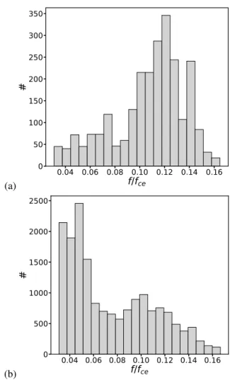
In Figs.3a,b, we show the normalized spacecraft frequency of the whistler waves identified using the peak and average BPF data. From Fig. 3a, we observe that most of the whistlers in the average BPF data are concentrated around 0.1 fce, which is

similar to previous observations in the solar wind (Tong et al.

2019a; Jagarlamudi et al. 2020). Meanwhile, from Fig. 3b, we

can observe that peak BPF data show a significant fraction of whistlers in the low normalized frequency (<0.05) range.

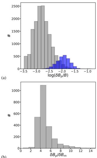
In Figs.4a,b, we show a histogram of the log of normalized peak amplitudes and the ratio of peak and average amplitudes corresponding to the whistlers. The method followed to estimate the approximate amplitude of the fluctuations that are associated with whistler waves is as follows: The spectral value of the iden-tified local maximum is multiplied with its respective frequency of the wave and the square root of this value is interpreted as the amplitude of the fluctuation. We note that δBprepresents the

peak amplitude calculated using the peak BPF data and δBm

rep-resents the average amplitude calculated using the average BPF data.

In Fig.4a, the blue histogram corresponds to intervals when whistlers are observed both in the peak and average BPF data, whereas the gray histogram corresponds to intervals when the

(a)

0.04 0.06 0.08 0.10 0.12 0.14 0.16

f/f

ce

0

50

100

150

200

250

300

350

#

(b)

0.04 0.06 0.08 0.10 0.12 0.14 0.16

f/f

ce

0

500

1000

1500

2000

2500

#

Fig. 3.Histogram of normalized frequencies of the whistler waves in

the average and peak BPF data. We show the normalized frequency of whistlers observed in average BPF data in panel a and the normalized frequency of whistlers observed in the peak BPF data in panel b.

whistlers are only observed in the peak BPF data, but not in the average. We observe a clear separation between the two distribu-tions. Normalized peak amplitudes of the whistlers, which are only observed in the peak band-pass data, are smaller (gray) than the ones which are observed in both peak and average BPF data (blue). We observe that most of the whistlers are of a low amplitude, and these whistlers are not observed in the average BPF data. We cannot deduce whether the low-amplitude whistlers are short-lived or not. However, we can observe that there is a considerable overlap between the gray and blue his-tograms, which suggests that there are whistlers which might be of a large enough amplitude to be visible in average BPF data, but they are very short-lived. Therefore, they are not visible in the average BPF data. We can also understand that most of the low normalized frequency whistlers observed in Fig.3b are of a low amplitude and that is the reason they are not visible in the average BPF data.

In Fig. 4b, we show the ratio of peak and average ampli-tude of the whistlers when whistlers are observed simultaneously in the average and peak BPF data. This relation is important in understanding the variability of the envelope of the whistler wave. From the plot, we observe that their ratios are concentrated between 3 and 7. This shows that when the whistler signatures are observed in both average and peak data, the ratios are nearly con-stant and there is no high variability. This leads us to conclude

V. K. Jagarlamudi et al.: Whistler wave occurrence and the interaction with strahl electrons (a)

3.5

3.0

2.5

2.0

1.5

1.0

log( B

p

/B)

0

500

1000

1500

2000

2500

#

(b)

Fig. 4.Histogram of peak and average amplitudes. Panel a: log of

nor-malized amplitudes of whistlers observed in the peak; blue corresponds to the data where whistlers are observed in both peak and average BPF, and gray corresponds to when the whistlers are observed only in the peak BPF spectra. Panel b: ratio of the peak and the average amplitude of spectra with whistler signatures.

that there might not be high variability in the whistler envelopes in our study when the whistlers are observed in both peak and average BPF data.

In Fig.5we show a histogram of whistlers as a function of the duration of their observation. The minimum whistler dura-tion is dependent on the resoludura-tion of BPF data; therefore, the minimum duration of the whistler is ∼0.87 s. For this study we use the whistlers observed in the average BPF data, as this provides the only approximate representation of how long the whistlers are continuously observed. Most of the whistlers in average BPF data are of a comparatively large amplitude and occur for a time that is long enough to be observed in average BPF spectra. We observe that 80% of the time, whistlers occur continuously for less than 3 s and the probability of observing whistlers continuously for a long duration (>30 s) is low. This shows that most of the whistlers occur intermittently, and the probability that whistlers occur for a long duration is low. There is an exponential decrease in the duration of the time whistlers are continuously observed. However, even when the whistlers appear continuously in the BPF data, it does not necessarily mean that a large whistler wave packet is present for such a long period. We believe that it could be a continuous occurrence of short duration whistler wave packets for a long time.

0

10

20

30

40

50

60

70

Duration (s)

10

0

10

1

10

2

#

Fig. 5.Histogram of the duration of whistler wave’s continuous

obser-vations in the average BPF data.

250 300 350 400 450 500 550 600 650

V

SW

(km/s)

0.0

0.2

0.4

0.6

0.8

1.0

1.2

1.4

%

of

w

his

tle

rs

Fig. 6. Occurrence rate of whistler waves as a function of the solar

wind bulk speed (Vsw). For each velocity bin, we show the fraction of

BPF data that have the signature of whistler waves.

We have presented some of the basic features of the observed whistler signatures. Now we explain how we studied the proper-ties of whistlers as a function of different physical parameters. First, we directly related the presence of whistlers to their observed conditions. Second, we related the plasma conditions to the duration of a consecutive whistler appearance. The first one gives information on the conditions when the whistlers are observed, while the second one gives important information on the differences in the conditions when whistlers are observed for a short duration compared to when they are observed continu-ously for a long duration. For these studies, we used the whistlers observed in the average BPF data, the reason is that they repre-sent the whole interval size unlike the whistlers that are only observed in the peak BPF.

In Fig. 6 we show the percentage of whistlers as a func-tion of solar wind bulk velocity, that is to say the number of whistlers in the velocity bin to the number of spectra available in the corresponding velocity bin, which takes the occurrence rate of different solar wind speeds into account. We observe that the lower the velocity of the wind, the higher the presence of whistler waves. A similar behavior is shown in the study ofJagarlamudi et al.(2020), where the authors show the anticorrelation between

10 20 30 40 50

Duration (s)

0.0018 0.0020 0.0022 0.0024 0.0026 0.0028 0.0030 0.0032

B/

B

(a) 10 20 30 40 50

Duration (s)

300 305 310 315 320 325 330

V

sw

(k

m

/s)

(b) 10 20 30 40 50

Duration (s)

260 270 280 290 300 310

N

p

(c

m

3

)

(c) 10 20 30 40 50

Duration (s)

0.06 0.08 0.10 0.12 0.14 0.16 0.18

|(B

B

)/

B

|

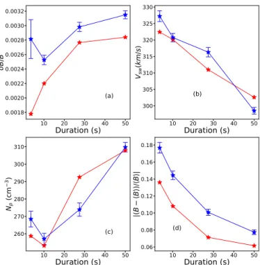
(d)

Fig. 7. Different properties of whistlers as a function of the duration

of their observations; blue and red correspond to the mean and median values, respectively. Panel a: normalized amplitude of whistler waves. Panel b: bulk velocity of the solar wind is shown. Panel c: density of the solar wind is shown. Panel d: magnetic field variations (|B−hBi

hBi |) are

shown. Error bars show the standard error (_√σ n).

the occurrence of whistler waves and the solar wind velocity. The authors explain the reason why for slower wind speeds, the conditions were better for the generation of whistlers through whistler temperature anisotropy instability (WTA) and whistler heat flux instability (WHFI).

We also looked into the relation between magnetic field gradients (such as drops, jumps and discontinuities) and the occurrence of whistlers. We used the ratio |B−hBi

hBi |as an

indica-tor for the magnetic field gradients, and we observe that nearly ∼80% of the time whistlers appear, the normalized magnetic field variations (|B−hBi

hBi |) are less than 30%, that is to say most

of the whistlers appear when there are not any large absolute magnetic field gradients. This guided us in concluding that large magnetic field gradients are not necessary for the occurrence of whistlers.

We also studied the relation between the occurrence of whistlers and the structures with sudden changes in the radial magnetic field orientation, called switchbacks (Bale et al. 2019;

Kasper et al. 2019;Dudok de Wit et al. 2020). For this, we used

the switchbacks identified in the work ofLarosa et al.(2021). We observed that only ∼15% of the switchbacks showed the pres-ence of whistler waves close to their boundaries or inside the structure.

In Fig. 7 we show the mean (blue) and median (red) of different plasma parameters when the whistlers are observed, as a function of their duration. We observe that the normal-ized amplitudes of the whistler waves which occur continuously are slightly higher compared to the whistlers of short duration. The velocity of the solar wind corresponding to the whistlers is relatively lower for the cases when the whistlers are observed continuously for a long duration. The density is higher for long

10

0

₁₀

1 c

10

2

10

1

10

0

|q

e

/q

0

|

Vasko et al 2019 (WFI), s/ c= 2 Vasko et al 2019 (WFI), s/ c= 0.5

Fig. 8.Normalized heat flux of the whistlers observed in the average

BPF data. We show the normalized heat flux (qek/q0) as a function of

electron core parallel beta (βekc), the dashed lines correspond to the

thresholds of whistler fan instability for∆s/∆c= 0.5 and ∆s/∆c = 2,

given byVasko et al.(2019).

duration whistlers. We also observe that normalized magnetic field variations (|B−hBi

hBi |) are lower when the whistler waves are

observed for a long duration. Similarly, we have also studied the variations in the radial magnetic field as a function of the dura-tion of the whistlers (not shown here). We observed that radial magnetic field variations were lower when the whistlers were observed for a long duration. This indicates that the probabil-ity of occurrence of long duration whistlers is lower when there are switchbacks. Long duration whistlers occur when the condi-tions are quiet. Now, in the following subsection, we look into the possible generation mechanism for the observed whistlers. 3.2. Whistler wave generation

Studies by Lacombe et al. (2014), Stansby et al.(2016),Tong et al.(2019a,b) andJagarlamudi et al.(2020) show that whistler heat flux instability is at work when whistlers are observed. For our case, in which we studied the whistlers which are observed closer to the Sun, we do not have an accurate estimate for the whistler heat flux instability threshold in the literature yet. The level of threshold is sensitive to variations in the densities of electron core and halo populations, and also their temperatures

(Gary et al. 1994), which vary with radial distance. Therefore,

we could not verify whether the whistler heat flux instability is at work or not. However, using the work ofVasko et al.(2019), where the instability thresholds were estimated by considering the electron core-strahl velocity distribution functions typical for the solar wind closer to the Sun (0.3–0.4 au), we could verify the probability of whistler fan instability (for oblique whistlers) working. For our study, we used the normalized heat flux values from the work ofHalekas et al.(2021). In Fig.8we present the normalized heat flux as a function of electron core parallel beta (βkc).

From Fig. 8 we infer that the whistler fan instability (for oblique whistlers) is probably at work, as the whistler intervals are around those thresholds (Vasko et al. 2019). However, fan instability is only pronounced for oblique whistlers and we do not have information on the angle of propagation. Therefore, it is important to know the angle of the whistler wave propagation with the mean magnetic field to properly identify for which cases the fan instability is at work. This will be one of the important goals for the future study.

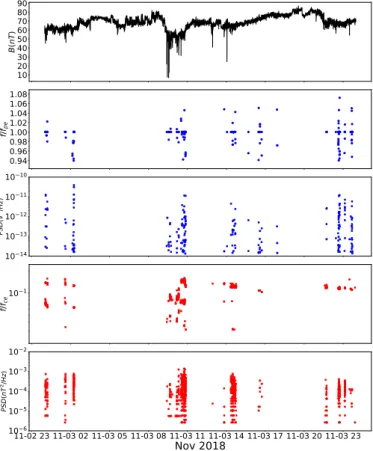
V. K. Jagarlamudi et al.: Whistler wave occurrence and the interaction with strahl electrons 10 20 30 40 50 60 70 80 90 B( nT ) 0.94 0.96 0.98 1.00 1.02 1.04 1.06 1.08 f/fpe 1014 1013 1012 1011 1010 PS D( V 2/Hz) 101 f/fce 11-02 23 11-03 02 11-03 05 11-03 08 11-03 11 11-03 14 11-03 17 11-03 20 11-03 23

Nov 2018

106 105 104 103 102 PS D( nT 2/Hz)

Fig. 9.Example of simultaneous observation of whistlers and Langmuir

waves in the PSP data. Panel 1: absolute magnetic field. Panel 2: nor-malized frequency of Langmuir waves with electron plasma frequency. Panel 3: spectral density of the observed Langmuir waves. Panel 4: normalized frequency of whistler waves with the electron cyclotron frequency. Panel 5: spectral density of whistler waves.

Recent study by Jagarlamudi et al. (2020) have suggested that whistler core and halo anisotropy instabilities might be at work when the whistlers are observed. For our study, only core electron anisotropy values are available and they are of a low resolution; therefore, we are not able to identify whether the whistler anisotropy instabilities are the source of our observed whistlers.

While analyzing the electron parameters, such as the den-sity and temperature measurements obtained from the QTN technique (Moncuquet et al. 2020), to study the conditions of whistler generation, we observed that for most of the times when the whistlers were observed, no halo or core temperatures were available corresponding to the whistler interval. This frequently observed behavior led us to probe the LFR data used for the elec-tron parameter estimation in the QTN technique. Interestingly, we observed that the LFR spectra showed the presence of a large spectral enhancement around the electron plasma frequency whenever there was a whistler wave during that time period. We identify these enhancements in LFR spectra as Langmuir waves, as all the jumps are centered around an electron plasma frequency (0.9–1.1 fpe). The simultaneous presence of whistlers

and Langmuir waves is similar to what has been reported in the study ofKennel et al.(1980) using the data from ISEE-3.

We identified that 85% of the time, intervals corresponding to whistlers in the average BPF showed the presence of Langmuir waves. A glimpse of this behavior can be seen in Fig.9, where the Langmuir waves normalized frequency and their PSD along with the whistlers normalized frequency and their PSD is shown in blue and red. From this plot, we can infer that there is a clear

correlation between the occurrence of whistlers (red dots) and Langmuir waves (blue dots) during this interval. These simul-taneous observations of whistlers and Langmuir waves give us a clue that there might be a common generation source for both the whistlers and Langmuir waves; therefore, we have to broaden our ideas as to potential whistler generation sources. An advanced study will be performed in the future using the waveform and high resolution particle data to accurately identify the source of the whistlers closer to the Sun.

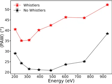
4. Whistlers and strahl electrons

In Fig.10we show the mean strahl pitch-angle width (PAW) of electrons when the whistlers are observed both in the average BPF data (red) and when the whistlers are not observed at all (black). We observe that the strahl PAWs are significantly larger in all the strahl energy ranges when the whistlers are observed. These observations point toward an interaction between whistler waves and the strahl electrons, which results in the observed broadening of the strahl electron population. The recent study

by Agapitov et al. (2020) identified the presence of sunward

whistlers along the switchback boundaries which could inter-act with the anti-sunward strahl electrons and scatter the strahl. However, in our study, we do not have any information on the direction of whistler wave propagation.

In Fig.11we show the difference in the strahl PAW between the intervals with whistlers observed in the average BPF and the intervals with no whistlers. We observe that the PAW is at least 12 degrees broader for sampled energies above 200 eV. The difference between PAW is the largest for the energies between 500 and 700 eV. A similar behavior was observed in the study ofKajdiˇc et al.(2016) at 1 au. An energy-dependent increase in strahl PAW is expected for the resonant interaction with narrowband whistler waves (Behar et al. 2020).

In Fig.12we show the mean strahl PAW of electrons corre-sponding to the whistlers by separating them on the basis of the duration of their consecutive observation. Type 1 corresponds to the family of whistlers which are observed for less than ∼3 s, and Type 2 corresponds to the family of whistlers which are observed for longer than ∼20 s. Interestingly, we observe that short duration whistlers show broader PAW than the long dura-tion whistlers. This distincdura-tion can be clearly seen in the energy range of 200–600 eV. This is an interesting result as we would expect the long duration whistlers to scatter the strahl broader than the short duration one. Instead, we observe in our study that shorter duration whistlers scatter the strahl more than the ones which are observed for a long duration.

In Fig.13a, we show the normalized amplitude of whistlers as a function of strahl PAW for electrons of energy 486 eV. We observe that there is no correlation (∼0.06) between the normal-ized amplitude of whistlers and strahl PAW. From the trends of normalized amplitudes of whistlers as a function of duration (see Fig.7a) and no correlation between the normalized amplitude of whistlers and strahl PAW, we can conclude that amplitudes of the waves may not be a reason for the observed differences between the strahl PAW of short duration (Type 1) and long duration (Type 2) whistlers shown in Fig.12.

In Fig. 13b, we show the normalized magnetic field varia-tions (|B−hBi

hBi |) as a function of strahl PAW for electrons of energy

486 eV. A positive correlation (∼0.54) between these two param-eters was found. We also found a similar correlation between the normalized magnetic field variations and the PAW of strahl electrons for other strahl energies (200–700 eV). Interestingly,

200 300 400 500 600 700 800 900

Energy (eV)

20

25

30

35

40

45

50

PA

W

(°

)

Whistlers

No Whistlers

Fig. 10.Mean strahl PAW of electrons as a function of electron energy

of whistler intervals observed in average BPF data (red) and of non-whistler intervals (black). Error bars show the standard error (_√σ

n).

200 300 400 500 600 700 800 900

Energy (eV)

12

14

16

18

20

22

PA

W

(°

)

Fig. 11. Difference in the mean strahl PAW of electrons of whistlers

observed in average BPF data and of non-whistler intervals as a function of electron energy.

short duration whistlers have relatively higher normalized mag-netic field variations than the long duration ones (see Fig.7d). These observations suggest that strahl PAW of electrons corre-sponding to the whistlers that are generated closer to the larger normalized magnetic field variations are broader and that the short duration whistlers are generated close to the larger normal-ized magnetic field variations, which can be connected to the result in Fig.12. Therefore, magnetic field variability might be one of the factors for the higher strahl PAW observed for the short duration whistlers compared to the long duration ones as observed in Fig.12.

The recent study byAgapitov et al.(2020) have shown the presence of oblique whistler waves closer to the Sun, and studies such asArtemyev et al.(2014,2016),Roberg-Clark et al.(2018),

Vasko et al. (2019),Verscharen et al. (2019) and Cattell et al.

(2020) have suggested that oblique whistlers scatter the strahl electrons better than the parallel ones. Therefore, our observa-tions may suggest that whistlers generated around the relatively higher magnetic field variations might be comparatively more

200 300 400 500 600 700 800 900

Energy (eV)

25

30

35

40

45

50

55

PA

W

(°

)

Type 1

Type 2

No Whistlers

Fig. 12.Mean PAW of whistlers separated on the basis of their duration

of observation and mean PAW of non-whistlers as a function of electron energy. Type 1 corresponds to the family of whistlers observed consec-utively for less than ∼3 s, Type 2 corresponds to the family of whistlers observed consecutively for more than ∼20 s, and the black curve corre-sponds to the non-whistler intervals. Error bars show the standard error (_√σ

n).

oblique than the ones which are generated around relatively low magnetic field variations.

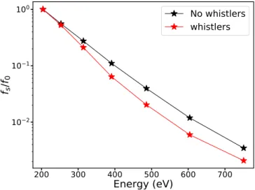
In Fig.14we show the parallel cut through the strahl electron VDF, that is to say the portion of the strahl velocity distribution function aligned with the magnetic field. We observe that for the non-whistler intervals, the distribution curves can be well represented by a Maxwellian VDF which forms a straight line in parameter space (Halekas et al. 2020;Berˇciˇc et al. 2020). On the other hand, for the whistler intervals, the distribution is curved compared to the non-whistler cases, corresponding to a Kappa distribution function better (see Fig. 11 inBerˇciˇc et al. 2020for a comparison between Maxwellian and Kappa fits to the strahl parallel VDF). The distribution of strahl electrons was observed to evolve with radial distance; in the near-Sun regions, the strahl was found to be close to a Maxwellian VDF, while further from the Sun it is better represented with a Kappa VDF. Kappa values were found to decrease with radial distance, which means that the relative density of high-energy tails increases as we move away from the Sun. A second suprathermal electron component, the halo, was found to be more important for larger distances from the Sun. The electron halo as well was found to be well represented by a Kappa distribution function (Maksimovic et al. 2005;Štverák et al. 2009). Our observational results reveal that whistler waves can affect the shape of the strahl VDF, and they could be one of the prominent mechanisms responsible for the radial evolution of strahl VDF.

In Fig. 15 we show the mean strahl parallel electron tem-peratures (Tks) corresponding to the whistlers observed in the

average BPF data and intervals with no whistlers. We find that mean Tks values are lower for whistler intervals compared to

their counterparts of non-whistlers with the same proton bulk velocity. There is more than a 10% decrease in the strahl tem-peratures corresponding to whistlers when compared to their counterparts corresponding to intervals with no whistlers. As shown byBerˇciˇc et al.(2020), an anticorrelation between Tksand

the solar wind velocity can be seen for non-whistler cases. How-ever, this anticorrelation between the Tksand solar wind velocity A9, page 8 of10

V. K. Jagarlamudi et al.: Whistler wave occurrence and the interaction with strahl electrons (a) 20 30 40

PAW (°)

50 60 70 80 90 0.002 0.004 0.006 0.008 0.010 0.012 0.014 0.016

(

B/

B)

100 101 (b) 20 30 40 50

PAW (°)

60 70 80 90 0.0 0.1 0.2 0.3 0.4 0.5 0.6 0.7

|(B

B

)/

B

|

100 101 102

Fig. 13. 2d histogram of the normalized amplitudes of whistler waves in

panel aand magnetic field variations corresponding to whistler waves in panel b as a function of the strahl PAW of 486 eV electrons. The black line and the dashed line correspond to the mean and median of the whistler wave’s normalized amplitudes and the magnetic field variations corresponding to the whistlers, respectively.

200

300

400

500

600

700

Energy (eV)

10

2

10

1

10

0

f

s

/f

0

No whistlers

whistlers

Fig. 14.Mean of the parallel cuts through the strahl VDFs ( fs)

normal-ized to the VDFs value at 200 eV ( f0). The black curve corresponds to

the non-whistler intervals, while the red curve corresponds the whistler intervals.

is not observed for the whistler intervals because these whistlers mainly appear in the slow solar wind.

During the presence of whistler waves, Tks appears to be

smaller than at other times. This observation together with the increase in strahl PAW shown in Fig.10, leads to the conclusion

250 300 350 400 450 500 550 600 650

V

sw

(km/s)

75

80

85

90

95

100

T

s

(e

V)

Whistlers

No Whistlers

Fig. 15.Mean strahl parallel temperatures (Tks) as a function of solar

wind bulk velocity, for whistlers observed in average BPF data (red) and for non-whistler intervals (black). Error bars show the standard error (_√σ

n).

that during the wave-particle interaction, the parallel strahl elec-tron momentum is converted to perpendicular momentum (Veltri

& Zimbardo 1993). Further analysis of waves and electron VDFs

are required to determine whether or not the total electron energy is conserved during this mechanism.

5. Conclusions

Our analysis of PSP DFB BPF data from the first perihelion has shown the presence of bursts of quasi-monochromatic elec-tromagnetic waves. These bursts are observed between 20 and 700 Hz. Despite only one component of the magnetic field data being available and even though the absence of accurate polar-ization measurements prevents us from accurately characterizing these waves, based on the knowledge from different studies at 1 au and the information from the cross-spectral data analysis, the bursts observed in the PSP’s DFB BPF data in the solar wind are interpreted as most likely due to the whistler waves. The statisti-cal study of these wave properties and their relation to the strahl electrons offer a unique opportunity in understanding the signifi-cance of the whistlers in strahl electron scattering. These results, in turn, help in gaining the insight into the solar wind energy transport, as strahl electrons carry the majority of the heat flux.

Our study has shown that whistlers occur highly intermit-tently and the spacecraft central frequencies of the waves are between fLHand 0.2 fce. The occurrence probability of whistlers

which are observed in the magnetic field is low (<2%), between 0.17 and 0.26 au whistlers are observed for less than 0.5% in average BPF data and around 1.5% of the time in peak BPF data. The occurrence of whistlers is highly dependent on the bulk velocity of the solar wind. We observe that the lower the velocity of the solar wind, the higher the occurrence of whistlers. A lower occurrence of whistlers suggests that even though whistlers might play a role in regulating the heat flux, they might not be able to completely explain the regulation of the heat flux in the solar wind.

Around 80% of the whistlers are observed for less than 3 s continuously. The occurrence of long duration whistlers (>30 s) is very low. We show that the velocity of the whistlers is lower for the cases when the whistlers are observed continuously for

a long duration. We also show that conditions are found to be quieter, that is to say magnetic field variations such as jumps, drops, and discontinuities are low when the whistler waves are observed continuously for a long duration.

In our study we observe the simultaneous occurrence of whistler and Langmuir waves, which confirms the idea that there might be a common source or a mechanism for the generation of these waves. An in-depth analysis on the reason for the simulta-neous presence of whistlers and Langmuir waves should be done in the future to find the common source for both the waves.

The strahl PAW of electrons in the strahl energy ranges are broader when the whistlers are observed, which suggests that whistlers are interacting with the strahl electrons and scatter-ing the strahl. Our observations also show that short duration whistlers scatter the strahl electrons better than the whistlers which are observed for a longer duration. The strahl parallel temperatures are observed to be lower for the intervals corre-sponding to the whistler waves than to the non-whistler intervals, which suggests that while whistlers are resonantly interacting with the strahl electrons and scattering them, they transfer the momentum from the parallel direction, leading to the decrease in strahl parallel temperatures for whistler intervals.

Whistler waves were found to have an effect on the shape of the parallel cut through strahl electron VDF. We therefore suggest that whistlers have an important role in the radial evo-lution of the strahl VDF and the formation of the Kappa-like halo observed farther from the Sun.

Acknowledgements.Authors thanks M. Liu for helpful discussion. The FIELDS experiment was developed and is operated under NASA contract NNN06AA01C. A.L., V.K., T.D., C.F., V.K.J. and C.R. acknowledge financial support of CNES in the frame of Parker Solar Probe grant. O.A. was supported by NASA grants 80NNSC19K0848, 80NSSC20K0697, 80NSSC20K0218. S.D.B. acknowledges the support of the Leverhulme Trust Visiting Professorship programme. Parker Solar Probe was designed, built, and is now operated by the Johns Hopkins Applied Physics Laboratory as part of NASA’s Living with a Star (LWS) program (contract NNN06AA01C). Support from the LWS management and technical team has played a critical role in the success of the Parker Solar Probe mis-sion. The data used in this study are available at the NASA Space Physics Data Facility (SPDF),https://spdf.gsfc.nasa.gov. Figures were produced using Matplotlib v3.1.3 (Hunter 2007;Caswell et al. 2020).

References

Agapitov, O. V., Dudok de Wit, T., Mozer, F. S., et al. 2020,ApJ, 891, L20 Alexandrova, O., Lacombe, C., Mangeney, A., Grappin, R., & Maksimovic, M.

2012,ApJ, 760, 121

Alexandrova, O., Krishna J., V., Rossi, C., et al. 2020, Nat. Commun., submitted [arXiv:2004.01102]

Artemyev, A. V., Vasiliev, A. A., Mourenas, D., Agapitov, O. V., & Krasnoselskikh, V. V. 2014,Phys. Plasmas, 21, 102903

Artemyev, A., Agapitov, O., Mourenas, D., et al. 2016,Space Sci. Rev., 200, 261 Bale, S. D., Goetz, K., Harvey, P. R., et al. 2016,Space Sci. Rev., 204, 49 Bale, S. D., Badman, S. T., Bonnell, J. W., et al. 2019,Nature, 576, 237 Behar, E., Sahraoui, F., & Bercic, L. 2020,J. Geophys. Res. Space Phys., 125,

e28040

Berˇciˇc, L., Maksimovi´c, M., Land i, S., & Matteini, L. 2019,MNRAS, 486, 3404 Berˇciˇc, L., Larson, D., Whittlesey, P., et al. 2020,ApJ, 892, 88

Boldyrev, S., & Horaites, K. 2019,MNRAS, 489, 3412

Case, A. W., Kasper, J. C., Stevens, M. L., et al. 2020,ApJS, 246, 43

Caswell, T. A., Droettboom, M., Lee, A., et al. 2020,https://doi.org/10. 5281/zenodo.592536

Cattell, C. A., Short, B., Breneman, A. W., & Grul, P. 2020,ApJ, 897, 126 Dudok de Wit, T., Krasnoselskikh, V. V., Bale, S. D., et al. 2020,ApJS, 246, 39 Feldman, W. C., Asbridge, J. R., Bame, S. J., Gosling, J. T., & Lemons, D. S.

1978,J. Geophys. Res., 83, 5285

Fox, N. J., Velli, M. C., Bale, S. D., et al. 2016,Space Sci. Rev., 204, 7 Froment, C., Krasnoselskikh, V., Agapitov, O. V., et al. 2020, in AGU Fall

Meeting 2020, AGU

Gary, S. P., Scime, E. E., Phillips, J. L., & Feldman, W. C. 1994,J. Geophys. Res., 99, 23391

Graham, G. A., Rae, I. J., Owen, C. J., et al. 2017,J. Geophys. Res. Space Phys., 122, 3858

Halekas, J. S., Whittlesey, P., Larson, D. E., et al. 2020,ApJS, 246, 22 Halekas, J. S., Whittlesey, P. L., Larson, D. E., et al. 2021,A&A, 650, A15(PSP

SI)

Hammond, C. M., Feldman, W. C., McComas, D. J., Phillips, J. L., & Forsyth, R. J. 1996,A&A, 316, 350

Hunter, J. D. 2007,Comput. Sci. Eng., 9, 90

Jagarlamudi, V. K., Alexandrova, O., Berˇciˇc, L., et al. 2020,ApJ, 897, 118 Jannet, G., Dudok de Wit, T., Krasnoselskikh, V., et al. 2021,J. Geophys. Res.

Space Phys., 126, e2020JA028543

Kajdiˇc, P., Alexandrova, O., Maksimovic, M., Lacombe, C., & Fazakerley, A. N. 2016,ApJ, 833, 172

Kasper, J. C., Abiad, R., Austin, G., et al. 2016,Space Sci. Rev., 204, 131 Kasper, J. C., Bale, S. D., Belcher, J. W., et al. 2019,Nature, 576, 228

Kennel, C. F., Scarf, F. L., Coroniti, F. V., et al. 1980,Geophys. Res. Lett., 7, 129 Lacombe, C., Alexandrova, O., Matteini, L., et al. 2014,ApJ, 796, 5

Larosa, A., Krasnoselskikh, V., Dudok de Wit, T., et al. 2021,A&A, 650, A3 (PSP SI)

Maksimovic, M., Zouganelis, I., Chaufray, J.-Y., et al. 2005,J. Geophys. Res. Space Phys., 110, A09104

Malaspina, D. M., Ergun, R. E., Bolton, M., et al. 2016,J. Geophys. Res. Space Phys., 121, 5088

Moncuquet, M., Meyer-Vernet, N., Issautier, K., et al. 2020,ApJS, 246, 44 Ogilvie, K. W., & Scudder, J. D. 1978,J. Geophys. Res., 83, 3776

Pagel, C., Gary, S. P., de Koning, C. A., Skoug, R. M., & Steinberg, J. T. 2007, J. Geophys. Res. Space Phys., 112, A04103

Pilipp, W. G., Miggenrieder, H., Mühlhaüser, K. H., et al. 1987a,J. Geophys. Res., 92, 1103

Pilipp, W. G., Miggenrieder, H., Montgomery, M. D., et al. 1987b,J. Geophys. Res., 92, 1075

Pulupa, M., Bale, S. D., Bonnell, J. W., et al. 2017,J. Geophys. Res. Space Phys., 122, 2836

Roberg-Clark, G. T., Drake, J. F., Swisdak, M., & Reynolds, C. S. 2018,ApJ, 867, 154

Scime, E. E., Bame, S. J., Feldman, W. C., et al. 1994,J. Geophys. Res., 99, 23401

Stansby, D., Horbury, T. S., Chen, C. H. K., & Matteini, L. 2016,ApJ, 829, L16 Štverák, Š., Maksimovic, M., Trávníˇcek, P. M., et al. 2009,J. Geophys. Res.

Space Phys., 114, A05104

Štverák, Š., Trávníˇcek, P. M., & Hellinger, P. 2015,J. Geophys. Res. Space Phys., 120, 8177

Tang, B., Zank, G. P., & Kolobov, V. I. 2020,ApJ, 892, 95

Tong, Y., Vasko, I. Y., Artemyev, A. V., Bale, S. D., & Mozer, F. S. 2019a,ApJ, 878, 41

Tong, Y., Vasko, I. Y., Pulupa, M., et al. 2019b,ApJ, 870, L6 Vasko, I. Y., Krasnoselskikh, V., Tong, Y., et al. 2019,ApJ, 871, L29 Veltri, P., & Zimbardo, G. 1993,J. Geophys. Rese. Space Phys., 98, 13325 Verscharen, D., Chandran, B. D. G., Jeong, S.-Y., et al. 2019,ApJ, 886, 136 Vocks, C. 2012,Space Sci. Rev., 172, 303

Vocks, C., & Mann, G. 2003,ApJ, 593, 1134

Whittlesey, P. L., Larson, D. E., Kasper, J. C., et al. 2020,ApJS, 246, 74 Zhang, Y., Matsumoto, H., & Kojima, H. 1998,J. Geophys. Res. Space Phys.,

103, 20529