HAL Id: hal-00302247
https://hal.archives-ouvertes.fr/hal-00302247
Submitted on 1 Jan 2003
HAL is a multi-disciplinary open access
archive for the deposit and dissemination of
sci-entific research documents, whether they are
pub-lished or not. The documents may come from
teaching and research institutions in France or
abroad, or from public or private research centers.
L’archive ouverte pluridisciplinaire HAL, est
destinée au dépôt et à la diffusion de documents
scientifiques de niveau recherche, publiés ou non,
émanant des établissements d’enseignement et de
recherche français ou étrangers, des laboratoires
publics ou privés.
Increasing the horizontal resolution of ensemble
forecasts at CMC
G. Pellerin, L. Lefaivre, P. Houtekamer, Christian Girard
To cite this version:
G. Pellerin, L. Lefaivre, P. Houtekamer, Christian Girard. Increasing the horizontal resolution of
ensemble forecasts at CMC. Nonlinear Processes in Geophysics, European Geosciences Union (EGU),
2003, 10 (6), pp.463-468. �hal-00302247�
Nonlinear Processes in Geophysics (2003) 10: 463–468
Nonlinear Processes
in Geophysics
© European Geosciences Union 2003
Increasing the horizontal resolution of ensemble forecasts at CMC
G. Pellerin1, L. Lefaivre1, P. Houtekamer2, and C. Girard3 1Canadian Meteorological Centre, Montreal, Canada
2Data Assimilation and Satellite Meteorological Division, Montreal, Canada 3Recherche en Prevision Numerique Dorval, Canada
Received: 20 August 2002 – Revised: 21 March 2003 – Accepted: 22 April 2003
Abstract. Ensemble forecasts are run operationally since
February 1998 at the Canadian Meteorological Centre, with outputs up to ten days. The ensemble size was increased from eight to sixteen members in August 1999. The method of producing the perturbed analyses consists of running in-dependent assimilation cycles that use perturbed sets of ob-servations and are driven by eight different models, mainly different in their physical parameterizations. Perturbed anal-yses are doubled by taking opposite pairs. A multi-model approach is then used to obtain the forecasts. The ensem-ble output has been used to generate several products. In view of increasing computing facilities, the ensemble pre-diction system horizontal resolution was increased to TL149 in June 2001. Heights at 500 hPa and mean sea-level pres-sure maps are regularly used. Charts of precipitation with the probability of precipitation being above various thresh-olds are also produced at each run. The probabilistic fore-cast of the 24-h accumulated precipitation has shown skill as demonstrated by the relative operating characteristic (ROC). Verifications of the ensemble forecasts will be presented.
1 Introduction
The ensemble prediction system is running operationally at the Canadian Meteorological Centre (CMC) since Febru-ary 1998, using 8 members of the SEF (Spectral Finite El-ement) model at resolution TL95 (Ritchie 1991). Adding the experimental runs, accomplished in development, the CMC ensemble prediction system has been running since January 1996. In August 1999, the ensemble size was dou-bled to 16 members. A different model, the Global Environ-ment Multi-scale (GEM), was then used for the additional 8 members (see Cˆot´e et al., 1998). Section 2 will describe the method used for this multi-model approach. With the increasing computational facilities at CMC in 2001, it was decided to increase the horizontal resolution of the set. Sec-Correspondence to: G. Pellerin (Gerard.pellerin@ec.gc.ca)
tion 3 will describe the results obtained when the horizon-tal resolution of the SEF ensemble members increased from TL95 to TL149, and the resolution of the GEM ensemble members increased from 1.875 to 1.2 degrees. No funda-mental changes to the methodology have been implemented since 1996, but as a result of these modifications, the scores have improved significantly. Section 3 will also describe the method used for verifications and the pertinence of the im-provement as compared to previous year validations. Sec-tion 4 will cover a short discussion and outline the future work planned.
2 Description of the ensemble prediction system
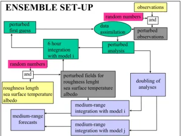
The ensemble method used at CMC is described in Houtekamer et al. (1996) and Lefaivre et al. (1997). The basis of the method is to produce perturbed analyses through data assimilation procedures. In order to do so, 8 parallel analysis cycles are run quasi-independently of the determin-istic operational analysis (TL199). In addition, the mean of the 8 analyses is calculated and then subtracted to that of the deterministic analysis. A fraction of this difference is then added to the original 8 perturbed analyses so that a total of 16 initial fields is obtained for the medium range forecasts (see Table 1). The characteristics of the perturbed cycles are summarised in Fig. 1.
First, each observation used to feed the analyses is per-turbed. For observations with multiple levels, such as ra-diosondes, the vertical correlations are taken into account by performing an eigenvector analysis of the vertical covari-ance matrix. Random numbers, drawn from a Gaussian dis-tribution with zero mean and unit variance, are then multi-plied by eigenvectors times the root of the eigenvalues (e.g. Houtekamer, 1993). For single- level observation, the pertur-bations are simply independent random numbers with zero mean and the variance appropriate for that observation. The random values are different for each independent piece of in-formation and are different from one perturbed cycle to the
464 G. Pellerin et al.: Increasing the horizontal resolution of ensemble forecasts at CMC
Table 1. Combination of modules for different model versions
SEF Add ops Convection/ GWD0 GWD0version Orography Number Time
(T149) analysis Radiation of levels level
1 yes Kuo/ Garand strong high altitude 0.3 σ 23 3
2 no Manabe/ Sasamori Strong low altitude 0.3 σ 41 3
3 no Kuo/ Garand weak low altitude mean 23 3
4 yes Manabe/ Sasamori weak high altitude mean 41 3
5 yes Manabe/ Sasamori strong low altitude mean 23 2
6 no Kuo/ Garand strong high altitude mean 41 2
7 no Manabe/ Sasamori weak high altitude 0.3 σ 23 2
8 yes Kuo/ Garand weak low altitude 0.3 σ 41 2
control mean Kuo/ Garand mean low altitude 0.15 σ 41 3
GEM Add ops Deep convection Shallow Soil moisture Sponge Number Coriolis
(1.2◦) analysis convection of levels
9 no Kuosym1 new <20% global 28 implicit
10 yes RAS2 old <20% equatorial 28 implicit
11 yes RAS2 old <20% global 28 implicit
12 no Kuosym1 old >20% global 28 implicit
13 no Kuosym1 new >20% global 28 explicit
14 yes Kuosym1 new <20% global 28 implicit
15 yes Kuosym1 old <20% global 28 implicit
16 no Kuosun3 new >20% global 28 explicit
0Gravity Wave drag (see McFarlane (1987) and McLandress and McFarlane (1993)) 1Deep convection stream (see Wagneur (1991))
2Relaxed Arakawa-Schubert (see Moorthi and Suraez (1992)) 3see Dastoor (1994)
Pellerin, G. et al., The CMC Ensemble Prediction System
7
ENSEMBLE SET-UP
and roughness length sea surface temperature albedo
medium-range forecasts
perturbed fields for roughness lenght sea surface temperature albedo random numbers observations and perturbed observations random numbers data assimilation perturbed first guess perturbed analysis 6 hour integration with model i medium-range integration with model i
doubling of analyses
medium-range integration with model j
Figure 1: Organisation chart of the ensemble set-up
Fig. 1. Organisation chart of the ensemble set-up.
other. The analysis scheme used is the Optimal Interpolation (O/I) technique (Rutherford, 1972), which has the advantage of being efficient computerwise (the weights for the innova-tions are calculated once for the control, using a cholesky
de-composition, and used for the 8 ensemble members as well). Second, each of the models used in the assimilation cy-cles, although based on the same spectral model (Ritchie, 1991) with a horizontal resolution of TL149 and a horizon-tal diffusion in ∇4, have different switches activated. These different configurations, used to produce the trial fields of each cycle, are described in the top half of Table 1. In ad-dition, some physical parameters are set with random values (horizontal diffusion, minimal roughness length over SST, time filter). Perturbations are also introduced in the surface forcing through modifications (gaussian perturbations) of the sea surface temperature, the albedo and the roughness length fields. The GEM models are only used for the forecasts.
Once a day, at 00:00 UTC, 10-day forecasts are produced using:
– 8 perturbed analyses, half of them obtained by adding a
fraction of the difference between the ensemble mean and the operational analysis (see 2nd column of Ta-ble 1), using the same model options as the ones used to produce the trial fields as detailed in top half of Table 1;
– the control run, obtained from an analysis with no
per-turbed observations and with intermediate model op-tions (the deterministic model keys are mostly used);
G. Pellerin et al.: Increasing the horizontal resolution of ensemble forecasts at CMC 465
Pellerin, G. et al., The CMC Ensemble Prediction System
8
Validation of ensemble forecasts (500 hPa) over NH DECEMBER 2000 2 3 4 5 6 7 8 9 10 1 2 3 4 5 6 7 8 9 10
Lead Time (days)
RM S errors agai nst anal yses ( d am) global (0.9) Mean-Lo (1.875) Spread-Lo Mean-Hi (1.2) Spread-Hi
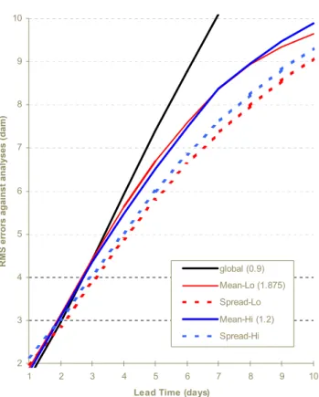
Figure 2: Verification (root mean square error) of height at 500 hPa over northern Hemisphere
for the low resolution ensemble (Solid red line) as compared to the High resolution ensemble (Solid blue line) and the deterministic model (solid black line); spreads in the ensemble are dashed lines.
Fig. 2. Verification (root mean square error) of height at 500 hPa
over northern Hemisphere for the low resolution ensemble (solid red line) as compared to the high resolution ensemble (solid blue line) and the deterministic model (solid black line); spreads in the ensemble are dashed lines.
– 8 perturbed analyses, half of them obtained by adding a
fraction of the difference between the ensemble mean and the operational analysis (see 2nd column of Ta-ble 1), using this time the GEM model with its own set of perturbations, detailed in bottom half of Table 1.
3 Verification results
By December 2000, a parallel run was set-up with the higher resolution ensemble. It was evaluated over the winter season (December to February) and gave acceptable results. It was then decided to pursue testing for a few months to assess the gain in the precipitation scores. The next sections will de-scribe verification scores for the RMS errors and Talagrand diagrams for the 500 hPa height field and for precipitation forecasts. The ROC curves provide a good representation of the quality of probabilistic precipitation forecasts (Mason, 1982). A comparison of ROC curves calculated for both low and higher resolutions will give a good indication of the im-provement of precipitation forecasts. This will be shown in the next sections.
3.1 RMS errors for the 500 hPa height field
The December 2000 verification for the two ensemble sets is seen in Fig. 2, where a series of Root Mean Square (RMS) er-rors of height at 500 hPa for Northern Hemisphere are shown. The solid line indicates the RMS error for the operational model (GEM 0.9◦ L28), while the thin blue and red lines, represent the ensemble mean RMS errors for the high and low resolution runs, respectively. The dotted lines repre-sent the spread of the ensembles (blue for high resolution). One would like to see the RMS errors for the ensemble mean smaller than for the high resolution model and the spread of the ensemble close to the ensemble mean error. Although af-ter 7 days, the scores of the high resolution ensemble are not as good as that of the low resolution one, the spread remains better for all forecast times. This was also the case for the month of July 2001 (not shown), the higher resolution en-semble had increased spread and reduced mean RMS errors throughout the 10 day period.
3.2 Talagrand diagrams for the 500 hPa height field To verify if the spread of an ensemble encompasses the ver-ifying analysis, Talagrand et al. (1997) proposed a statisti-cal method for displaying bias and dispersion within the en-semble. The so-called Talagrand diagrams are obtained by checking where the verifying analysis usually falls with re-spect to the ensemble forecast data (arranged in increasing order at each grid point). The first (last) bin is selected if the analysed value is lower (higher) than any of the values in the ensemble.
Since all perturbations are intended to represent equally likely scenarios, this distribution should be flat. Several com-mon problems can be diagnosed from the diagrams:
– a U-shape diagram is obtained if the spread in the
en-semble is typically too small;
– if the spread in the ensemble is too big one obtains an
n-shape (highest in the middle);
– if the diagram is asymmetric the model has a bias to one
side. An L-shape would correspond to a warm bias for the model.
Operationally, these diagrams are produced every month. For our comparison we show the low (TL95) and high res-olution (TL149) diagrams for the 500 hPa (global coverage) in Figs. 3 and 4 respectively. These diagrams are for all lead times of the month of February 2001. It is encouraging to see that the diagrams display nearly flat distributions with no marked systematic biases, except a slight warm bias which does not seem to have changed with the increase in resolu-tion. It is true that there is too much spread at day 1, espe-cially for the high resolution ensemble. We think that this may be due to the perturbations of the observations which were set to high (factor 1.8) during the analysis cycles.
466 Pellerin, G. et al., The CMC Ensemble Prediction SystemG. Pellerin et al.: Increasing the horizontal resolution of ensemble forecasts at CMC
9 Figure 3:Talagrand diagrams for height at 500 hPa over global area for February 2001 for lead times from 24 to 240 hours, for low resolution model (192x96).
Fig. 3. Talagrand diagrams for height at 500 hPa over global area for
February 2001 for lead times from 24 to 240 h, for low resolution model (192 × 96).
3.3 Relative Operating Characteristic curves for precipitation
The Relative Operating Characteristic (ROC) curves have been proposed by Mason (1982) as a verification measure for ensemble forecasts. The method is based on ratios that measure the proportions of events and non-events for which warning can be provided. The ratios provide estimates of the probabilities that an event will be for-warned (hit-rate) and that an incorrect warning will be provided for a non-event (false-alarm). In a ROC curve, the hit rate is shown as a function of the false alarm rate. The surface under the curve gives a good indication of the performance of the system. It is worth noting that a ROC area of 0.5 is the no-skill level, with the arbitrary value of 0.7 being accepted as the lower limit of usefulness (see Mason, 1982). The detection of pre-cipitation events (Hit rate) and non-events are obtained from a data set of nearly 160 stations distributed across Canada. These statistics are tabulated every 3 months and have been carried since early 1997. Figure 5 shows the ROC curves for the low (a) and high (b) resolution ensemble sets. These
re-Pellerin, G. et al., The CMC Ensemble Prediction System
10
Figure 4: Talagrand diagrams for height at 500 hPa over global area for February 2001 for lead
times from 24 to 240 hours, for high resolution model (300x150).
Fig. 4. Talagrand diagrams for height at 500 hPa over global area for
February 2001 for lead times from 24 to 240 h, for high resolution model (300 × 150).
sults are for the 5 mm threshold at 4 lead times (day 1, day 4, day 7 and day 10). They were calculated for the 3 month pe-riod starting in December 2000 and ending February 2001. The area under the curves (see Table 2) shows that both sets demonstrate skill up to 10 days and that the high resolution is better at all lead times.
Increasing the resolution to improve on the precipitation forecasts was also demonstrated with the ECMWF ensemble system (Buizza et al., 1998). Interestingly this relative gain is about the same as that obtained when the ensemble pre-dictions system was increased in size from 8 to 16 members, which is shown under LOW(8) for 8 members. Generally speaking, Table 2 shows that an increase in ensemble resolu-tion has a positive impact on the ensemble skill, due mostly to better topography related precipitation forecasts.
It is interesting to plot the variation of the areas as a func-tion of the lead time. Figure 6 shows the plot of the low resolution scores (in dashed red) along with the high reso-lution scores (in solid black). As mentioned earlier, the im-provement is apparent up to day 7, marginally so there after. After re-sampling our scores into shorter periods (10 days),
G. Pellerin et al.: Increasing the horizontal resolution of ensemble forecasts at CMC 467
Pellerin, G. et al., The CMC Ensemble Prediction System
11 Figure 5: Relative Operating Characteristic curves for 5mm threshold for Winter 2000-01 (Dec-Jan-Feb) for low resolution models (192X96) in a) and high resolution models (300X150) in b).
5mm - ROC Winter Season (D-J-F)
0.65 0.7 0.75 0.8 0.85 0.9 1 2 3 4 5 6 7 8 day(s)9 10 Areas
Figure 6: Comparison of ROC curves for the 5mm threshold for Winter 2000-01 (Dec-Jan-Feb) for high resolution models in solid black and low resolution models in dashed red.
Fig. 5. Relative Operating Characteristic curves for 5 mm
thresh-old for Winter 2000–01 (Dec–Jan–Feb) for low resolution models (192 × 96) in (a) and high resolution models (300 × 150) in (b).
Table 2. Comparison of ROC areas between high and low
resolu-tion (16 and 8 members)
high low (16) low (8)
day 1 0.892 0.887 0.870
day 4 0.824 0.798 0.781
day 7 0.772 0.751 0.730
day 10 0.719 0.716 0.683
we find the null hypothesis using student-t confidence level is rejected at 65% at day 1, 75% at day 4, 85% at day 7 but ac-cepted beyond day 8. It is clear that both sets differ slightly at the beginning, due to the highly deterministic nature of short lead time. The higher resolution forecasts show an in-crease in skill up to day 7, afterward both sets move towards the climatological threshold. There is a fair amount of sea-sonal variations in these ROC scores and it is also interesting to plot the annual variations with time. Figure 7 shows four consecutive winter scores for the 5 mm threshold. The 4 con-secutive years are; 1997–1998 in blue (8 members), 1998– 1999 in grey (8 members), 1999–2000 in green (16 mem-bers) and 2000–2001 in red (16 memmem-bers), all of which are computed from the common grid of 192 × 96 points. The comparison with the previous plots indicate that the annual variability is as great as the improvement obtained by the in-crease of resolution to 300 × 150 grid points.
The winter verifications (Figs. 6 and 7) show that forecasts have utility up to and even beyond day 7. These conclusions are similar for the 2 and 10 mm thresholds, the 25 mm thresh-old is not verified because of the sample being too small.
4 Future work
The first priority is to make full use of the 16-member en-semble, extending the generation of our products in terms of probabilistic forecasts. Probabilities thus obtained will be used in the production of worded forecasts up to day 10. Ver-ification methods will also include the Probability
Distribu-Pellerin, G. et al., The CMC Ensemble Prediction System
11 Figure 5: Relative Operating Characteristic curves for 5mm threshold for Winter 2000-01 (Dec-Jan-Feb) for low resolution models (192X96) in a) and high resolution models (300X150) in b).
5mm - ROC Winter Season (D-J-F)
0.65 0.7 0.75 0.8 0.85 0.9 1 2 3 4 5 6 7 8 day(s)9 10 Areas
Figure 6: Comparison of ROC curves for the 5mm threshold for Winter 2000-01 (Dec-Jan-Feb) for high resolution models in solid black and low resolution models in dashed red.
Fig. 6. Comparison of ROC curves for the 5 mm threshold for
Winter 2000–01 (Dec–Jan–Feb) for high resolution models in solid black and low resolution models in dashed red.
Pellerin, G. et al., The CMC Ensemble Prediction System
12
5mm - ROC Seasonal Variation (D-J-F)
0.65 0.7 0.75 0.8 0.85 0.9 1 2 3 4 5 6 7 8 days 9 10 Areas 1997+98 1998+99 1999+00 2000+01
Figure 7: Comparison of ROC curves at the 5mm threshold for Winter season starting 1997-1998 in blue, 1998-1999 in grey, 1999-2000 in green and ending 2000-2001 in red. (All low resolution).
Fig. 7. Comparison of ROC curves at the 5 mm threshold for Winter
season starting 1997–1998 in blue, 1998–1999 in grey, 1999–2000 in green and ending 2000–2001 in red. (All low resolution).
tion Function, as proposed by Wilson et al. (1999).
Second, at some point in the near future, the OI code will be replaced by an equivalent resolution ensemble Kalman filter. Since 1996, a great deal of effort has been concen-trated on the development of an ensemble Kalman filter (see Mitchell and Houtekamer, 2000; Houtekamer and Mitchell, 2001; Mitchell et al., 2002). It is currently possible to assim-ilate a full set of observations with one of the latest version of the GEM model. The ability of the Kalman filter to pro-vide the analyses for the medium-range ensemble prediction system is being examined.
Third, exchanges with NCEP have started in order to produce “grand ensemble” products. This collaboration is likely to be continued.
References
Buizza, R., Petroliagis, T., Palmer, T. N., Barkmeijer, J., Hamrud, M., Hollingsworth, A., Simmons, A., and Weddi, N.: Impact of model resolution and ensemble size on the performance of an ensemble prediction system, Q. J. R. Meteorol. Soc., 24, 1935– 1960, 1998.
Cˆot´e, J., Gravel, S., M´ethot, A., Patoine, A., Roch, M., and Stan-iforth, A.: The Operational CMC/MRB Global Environmental
468 G. Pellerin et al.: Increasing the horizontal resolution of ensemble forecasts at CMC
Multiscale (GEM) Model: Part I – Design Considerations and Formulation, Mon. Wea. Rev., 126, 1373–1395, 1998.
Dastoor, A. P.: Cloudiness parameterization and verification in a large-scale atmospheric model, Tellus, 46A, 615–634, 1994. Houtekamer, P. L.: Global and local skill forecasts, Mon. Wea. Rev.,
121, 1834–1846, 1993.
Houtekamer, P. L., Lefaivre, L., Derome, J., Ritchie, H., and Mitchell, H. L.: A system simulation approach to ensemble pre-diction, Mon. Wea. Rev., 124, 1225–1242, 1996.
Houtekamer, P. L. and Mitchell, H. L.: A Sequential Ensemble Kalman Filter for Atmospheric Data Assimilation, Mon. Wea. Rev, 129, 123–137, 2001.
Lefaivre, L., Houtekamer, P. L., Bergeron, A., and Verret, R.: The CMC Ensemble Prediction System. Proc. ECMWF 6th Work-shop on Meteorological Operational Systems, Reading, U.K, ECMWF, 31–44, 1997.
Mason, I.: A model for the assessment of weather forecasts, Aust. Meteor. Mag., 30, 291–303, 1982.
McFarlane, N. A.: The effect of orographically excited gravity wave drag on the general circulation of the lower stratosphere and tro-poshere, J. Atmos. Sci., 44, 1775–1800, 1987.
McLandress, C. and McFarlane, N. A.: Interactions between oro-graphic gravity wave drag and forced stationary planetary waves
in the winter Northern Hemisphere middle atmosphere, J. Atmos. Sci., 50, 1966–1990, 1993.
Mitchell, H. L. and Houtekamer, P. L.: An Adaptive Ensemble Kalman Filter, Mon. Wea. Rev., 128, 416–433, 2000.
Mitchell, H. L., Houtekamer, P. L., and Pellerin, G.: Ensemble Size, Balance and Model-Error Representation in an Ensemble Kalman Filter, Mon. Wea. Rev. 130, 2791–2808, 2002.
Moorthi, S. and Suarez, M. J.: Relaxed Arakawa-Schubert: A pa-rameterization of moist convection for general circulation mod-els, Mon. Wea. Rev., 120, 978–1002, 1992.
Ritchie, H.: Application in the semi-Lagrangian method to a multi-level spectral primitive-equations model, Quart. J. Roy. Meteor. Soc., 117, 91–106, 1991.
Rutherford, I. D.: Data assimilation by statistical interpolation of forecast error fields, J. Atmos. Sci., 29, 809–815, 1972. Talagrand, O., Vautard, R., and Strauss, B.: Evaluation of
proba-bilistic prediction systems, Proceedings, ECMWF Workshop on Predictability, 1997.
Wagneur, N.: Une ´evaluation des sch´emas de type Kuo pour le param´etrage de la convection, Msc Thesis, UQAM, 76, 1991. Wilson, L. J., Burroughs, W. R., and Lanzinger, A.: A Strategy
for Verification of Weather Element Forecasts from an Ensemble Prediction System, Mon. Wea. Rev., 127, 956–970, 1999.