Commuting, Ricardian rent and house price appreciation in cities with dispersed employment and mixed land-use

W' ' MITLIBRARIES

Digitized

by

the

Internet

Archive

in

2011

with

funding

from

Boston

Library

Consortium

Member

Libraries

mB3i

,>^

^

M415

3^

Massachusetts

Institute

of

Technology

Departnnent

ot

Economics

Working

Paper

Series

COMMUTING,

RICARDIAN

RENT

AND

HOUSE

PRICE

APPRECIATION

IN

CITIES

WITH

DISPERSED

EMPLOYMENT

AND

MIXED

LAND-USE

William

C.

Wheaton

Working

Paper

02-35

March

2002

Room

E52-251

50

Memorial

Drive

Cambridge,

MA

02142

This

paper

can

be

downloaded

without

charge from

the Social

Science

Research Network Paper

Collection at

I

MASSACHUSEHS

INSTITUTE I

_OFTECHNOLOGY_

JAN

2

1

2003

Draft:

March

23,

2002

Commuting,

Ricardian

Rent

and

House

Price

Appreciation

in

Cities

with

Dispersed

Employment

and

Mixed

Land-Use

By

William

C.

Wheaton

Department of

Economics

Center

for

Real

Estate

MIT

Cambridge,

Mass

02139

wheaton@mit.edu

Originallypresentedatthe

2001 meeting of

the

Asian

RealEstate Society,

August

1-4,

2001

Abstract:

Commuting,

Ricardian

Rent

and

House

Price

Appreciation

In

Cities

with

Dispersed

Employment

and

Mixed

Land

Use

For

centuries,cities

have been

modeled

asgeographically centered

markets

in

which

locational scarcitygeneratesRicardian

Land

Rent,that inturn increases

over time

as citiesgrow. This paperfirstpresents

some

empirical evidencethat this isnotthe case: inflation-adjustedlocational rent

does

not

mcrease over

time

-

despite

enormous

urban

growth.Rather thantrying toexplainthistendency withina "monocentric"

framework,

this

paper

developsa

model where

jobs

and

commerce

can

be

spatiallyinterspersed

with

residences,

under

certain

economic

conditions.

The

paper

presents

new

empirical evidencethat

such job

dispersal

does

characterize atleast

US

cities.

The

comparative

statics

of

this

model

are

much

more

consistentwiththe data

-

accommodating

extensive

urban growth

withhttleor

no

increasein

commuting

and

Ricardian Rent.

I.

Introduction

Sincethe 19'*^ _{century, the}

_dominant

_view

_{of urban}

_{landuse has}

_{been based}

_on

_the

Ricardianrent,monocentriccity

model.

Inthis

model,

transportationfrictions for

commuting

or

commerce

generatea rent"gradient"

between

acitycenter

and urban

periphery.Thisentiregradient increases ascities

grow

inpopulation

because

travel distances

expand

and

speedsdeteriorate. Implicitly, this

model

is

behind

the

widespread

behef

thaturban housingprices(andrents)

grow

over tamesignificantly fasterthan

inflation. Increasedlocation"scarcity"

makes

real estateassets a

"good"

investment.

This

paper

has

two

objectives.

The

first isto

review

a range

of

empiricalevidence

thatsuggeststhisvision

of urban

form

islargelyincorrect.

Over

time, in

most

cities, real estaterents

and

assetprices

grow

httle

more

thaninflation.This isconsistentwiththe recentexperiencein

US

cities,

where

commuting

durations

have

not

worsened

inthelast

30

years, despite

huge

increases inpopulation

and

VMT.

Finally, recently released data

on

the spatialdistribution

of

jobs(by place

of work)

suggestthatfirms

and

residencesare

remarkable

well interspersed.

The

factssimply

do

notfita"monocentric"

model

-

nor

do

they supportits

comparative

staticswithrespect togrowth.

The

second

objectiveisto

develop

averysimply

model

of urban

spafialstructurethat doesfitthesefacts.

The

model

makes

many

simplifyingassumptions,

and

has

few

embellishments, butitcan

generatecity

forms

thatare consistentwiththedata

-

and which

do

yieldlittleor

no

growth

in real estatevaluesascities

expand

inpopulationoverthelongrun.This

model

hasfive

key

features.

•

Mixing

orinterspersedland

use

occursiflandisallocated toresidences or

commerce

inproportiontotheirrentratherthantothestrictlyhighestrent. •

The

rent foreachuse,

and

thusthe degree

of mixing depends

on

tradingoffthe

benefits

of

some

economic

agglomeration factorwiththeease

of

travel.

• Travelpatterns are

determined

with

mixed

landuse,

and

Solow

typecongestionis introduced.

Congestion

ishighestwith ftiUycentralized

employment

and

becomes

negligible as

commerce

isfijllydispersed

and

evenly

mixed

withresidences. • Inacitywith highly dispersed

employment

there turnsoutto

be

littleor

no

Ricardianrent

"gradienf

,incontrasttoa citywithcentralizedemployinent.

•

As

acitywithdispersed-

employment

increasesinpopulation

and

grow

spatially, thereis less,

and

in

some

cases

no

increasein

commuting

and

Ricardianrent,

againinsharpcontrasttoacitywithcentralized

employment.

The

paperisorganized asfollows.

The

nextsectionreviews a range

of

empirical

evidence

aboutboththe

growth

inreal estatevalues,

and

thespatialdistribution

of

jobs

and

people withincities.

The

followingsectionprovidesan

example of

how

dispersed

employment

and

mixed

landuse

can

generate congestedtraffic flows

between

firms

and

residences. Inthefourth section,thesetravelcostsare

used

togenerateequilibrium Ricardianrent

and

wage

gradients forboth firms

and

households. In sectionfive,the

model

isclosed,

by

incorporating

an

"idiosyncratic"auctionfiinctionthatallocates land

use based

on

therelative

magnitude of

Ricardianrents

from

the

two

uses.

The

sixth

withthelevel

of urban

agglomeration,thelevel

of

transportationinfrastructure,

and

population growth. Section nine then

compares

how

land rents

change

with population

growth

in citieswithfully dispersed

employment,

as

opposed

totraditional

monocentric

cities.

The

finalsectionconcludes with a longUst

of

suggested futureresearch

11.

Empirical Evidence.

The

firstevidencethat real estatevalues

might

notrisecontinually in realterms

comes

from

the

unique

Eicholtz [1999]repeat-salepriceindexforhousinginthecity

of

Amsterdam:

from 1628 through

1975.

The

deflated series inFigure 1

shows

no

obvious

trend,

and

statisticaltests

confirm

its stationarity. Thus, during almost

350

years,the

greater

Amsterdam

areahas gro\yninpopulation

and

jobs

by

1

200%

without

having

house

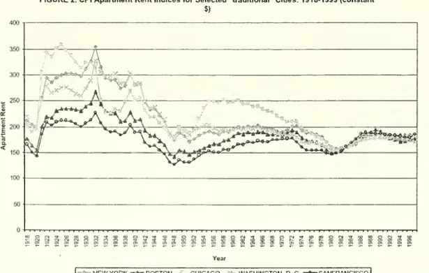
pricesrise fasterthaninflation.

Figures2

and

3

show

the longeststanding

US

series

on

residential

markets

-apartmentrents

from

the

US

Commerce

Department's

CPI

repeat

sample

survey, fri

Figure2,theindicesfor five"traditional"citiesare

shown,

whileinFigure3,the indices forthree

"newer"

citiesaredisplayed(constantdollars).

None

seems

to

have an

upward

trend,

and

theseriesforthe

"newer"

citiesactually

have

significant

downward

trends. If theseriesare

examined

over

just the

post-war

period

(1946-1999),

the

same

statistical

conclusionshold .

Over

these 81 years, thecitiesin this

sample

had

population

growth

(in theirmetropolitanareas)

of

between

110%

(New

York)

to

2100%

(Houston).

The

fmal data

examined

isthe

much

more

recent

OFHEO

repeat sales priceindex

for

US

single-family housing.

Here

again. Figure

4 shows

deflated prices forfiveolder cities,while Figure 5

does

sofor5

newer

areas:

from

1975

tothe present, hi four

of

the fiveoldercity series,there

does appear

to

be an

upward

trendinprices,butinthe

newer

citiesthereisnone. Infact,thisis

vaUdated

statistically,althoughthetimeseriesbehavior

of

the

two

groups

of

citiesisquitedifferent .Itisimportanttoseethatthe rentseries in

Figure3

show

asimilar

upward

trendas

do

prices

-

if

examined

from 1975

-

an

artifact largely

of

the shorttimeframe.

In recent years, therehas

been

anunrelated,but

growing

empiricalliteraturethat

suggests

employment

isfar

more

dispersedthan previouslythought. Mills[1972]

To

teststationarityfirstrequiresidentifying theunderlyingbehaviorofa series.

To

dothis,thefollowing

modelisestimated:?yi= ao

+

ai?yt.|...+By,+dt +et .

An

augmented"F"statisticisusedtodetermineif13

anddarecollectivelysignificant. If so,thenthe"t" statisticofd ascertainswhetherthe seriesisstationary. If arandom walk modelcannotberejected,thenthe"t"statisticonao ascertainswhetherthereissignificant "drift".FortheDutchseries,the"F"testpassesthe

5%

levelusing theaugmentedDickey-Fullercriteria,

but the trendhasa "t" statisticof only.6.

The same "F"statisticisgenerallylessconclusiveaboutwhethertheCPI dataisarandomwalkor

mean

reversionary.Theadditionofa

mean

reverting trendadds explanatorypowerinalloftheseries,but often onlyat 10-20%significance.Inoldercities,thetrend"t" statisticsrangefrom1.6to-1.4.Inthe

new

cities theyrangefrom-1.2 to-3.2.Inallcases, thevalueof oisnotsignificantfromzero

One

mustplace limitedcredenceinany timeseries testswith only25observations.Still,inall5older city series

mean

reversionisstatisticallysignificant, andinfouroffivethe trendsaresignificantatthe

5%

level. Inthe

new

cities,therandom walk modelcannotberejectedandthereisnosignificantdrift.If a

estimated

employment

aswellaspopulationdensity gradients,

and claimed

thatjobs

were

indeed

much

more

dispersed thanina

monocentric model.

More

recentresearch continuesto

show

that

employment

in

metropohtan

areas

around

theworld,isboth

dispersing

and

in

some

casesclusteringintosubcenters [Guiliano

and

Small, 1991;

McMillen-Macdonald,

1998]. Finally,there isequally

ample

evidence

of

thespatial variation in

wage

rates,

which

isnecessaryto

accommodate

job

dispersal [Eberts, 1981;

Madden,

1985;Dilanfeldt, 1992;

McMiUen-SingeU,

1998;

Timothy-

Wheaton,

2001].

A

more

detailedanalysis

of

jobdispersalhasrecently

become

possiblewiththe release

of

Commerce

Department

information

on

employment

atplace

of

work

-

by

Zip

Code

- asreportedin

Glaeser-Kahn[2001].

With

zip

code

leveldata, itispossibleto

constmctthecumulativespatialdistribution

of

employment

aswellaspopulation

-

from

the "center"

of each

MSA

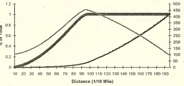
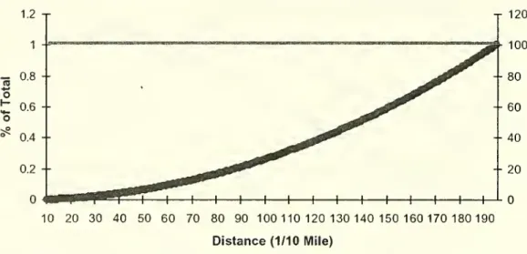
outward. Thisis

shown

inFigures6

and

7,forthe

two

areas in

the

US

that areheld

up

as representing "traditional" as

opposed

to"newer''cities:the

New

York

and

Los

Angeles

CMSAs.

While

employment

is slightly

more

concentrated than populationin

New

York,

thecloseness

of

the

two

distributionsis

unexpected

-

asis the remarkablesimilarityto

Los

Angeles

-

where

the

two

distributions arevirtually identical.

Itiseasyto

constmct

a simple

measure

of

how

"concentrated"thespatial

distributionsare inFigures

6 and

7.

One

takes the integral

of

the distribution

-

up

to (say) the

95%

point

and

then divides

by

thedistanceatthatpoint.Citiesthatare"flilly"

concentratedatsinglecentralpoint

have

avalue

of

unity,whilecitieswithan

even

distribution

have

a value

of

.5.

A

citywithvirtually all

employment

orpopulationatits

"edge"

would

have

a valuethatapproacheszero,hiFigure8,the value

of

this

measure

forbothpopulation

and

employment

is

shown

for 1

20

MSAs

(or

CMSAs).

Across

these

areas,the

measure of

population concentrationvaries

from

about.5to .75

depending

on

how

dense

and

spread out populationis.

What

is

remarkable

isthe extremelyclose correlation

between

the

two

measures

(R

=

.72). Citiesin

which

population isspread out

-

jobsare aswell

-

and

vice versa.

A

tme

"monocentric"

city

would

have

an

employment

valueof

something

like .8

and

a populationvalue

of

lessthan.5.

There

are

no

citieslike this.

Finally,the

US

National Personal Transportation

Survey

reportsthataverage

urban

commuting

durationsfell

from

22.0minutesin

1969

to20.7minutesin 1995,

despite thefactthat

VMT

grew

far fasterthanthe rathersmallincreasesin

Lane

Miles

of

Capacity.

Avoiding any

aggregationbias,

Gordon

and Richarson

[2001] report that

average

commuting

durationsinthe

Los Angeles

CMSA

have remained

unchanged from

1967

to

1995

-

despitea

65%

increaseinpopulation,

and an

85%

increaseinjobs.

What

explainsboththeremarkable abihty

of metropohtan

areas toabsorb growth,

and

ahigh degree

of

intermixed land use?Inthe followingsections,a

model

is

developed

which

brings togethera

number

of

previousideasintheUterature.

Following

White

[1976, 1988],

and

Ogawa

and

Fujita [1980], the

model

motivates

employers

toseek proximitytoresidencesinorderto

lower

the

commuting

and hence

wages

thatthey

pay

workers.

From

Helseley-Sulhvan

[1991],

and

Anas-Kim

[1996], the

model

introducesa

spatialagglomerationfactorfor firms,

which

provides

some

rationale forcentralization. Finally,

Solow-type

[1973]transportationcongestionisintroducedfor thefirsttimein

such models.

What

makes

the synthesis

of

theseideas analytically tractable isthe

mtroduction

of "mixed"

landuse

-

firms

and

residences

can

"jointly"

occupy

landatthe

same

location

-

depending

on

therelative

magnitude of

theirlandrents.

in.

Commuting

with

Dispersed

Employment

and

Mixed Land

Use

Like atraditional

monocentric

city,thecity

modeled

herewill

be

circular

and

have

a transportationtechnologythatonly allows

inward

radial

commuting.

The

only

distinguishing feature

of

landisthusitsdistance (t) fi^omthe geographiccenter

of

the city.

Land

that isnotvacantis

occupied

either

by

household

residencesor

by

the firms

that

employ

them.

At

each

location(t),the fraction

of

land

used

by

firms is F(t),

and

that

by

householdsis l-F(t).

The

functionF(t)will

be

discussed later.

For

now,

itissimply specified asa

mapping

from

tintothezero-oneinterval.

A

simplificationinthe cuirent

model

will

be

the

assumption

thatindividuals

consume

a fixed

amount

of

landspace,bothattheirplace

of

employment

(qr )aswellas

atthe location

of

theirresidence _(qh ).hi

most

modem

cities,

workplace

land

consumption

isfarsmallerthanresidential (qf

<

qh ),butthisisonly

an

observation

and

isnotnecessaryforthe

model

athand.

Allowing

density to

be endogenous

complicates

the

model,

butprobably

does

not

change

thequahtative conclusions derivedhere.In

any

case, itwill

be

one of

many

suggestedfiitureextensions.

With

fixeddensityatboth residence

and

workplace,e(t)

and

h(t)are

defmed

as

thecumulative

number

of workers

orhouseholds

who

hve

up

tothe

distance

t.

Using

the

F(-)fijnction,theseare:

e(t)= o'?2pxF(x)/qf

dx

,^ (1)

h(t)= o'i^2px[l-F(x)]/qhdx (2)

The

spatialdistribution

of

employment

and

householdswill

have

anouter

"edge"

orlimit.

No

jobsexist

beyond

the distance bf

and

no

households

beyond

thedistance

bh-The

following

boundary

conditions

on

e(t)

and

h(t)areobvious,

where

the

equaUty

between

totaljobs

and households

is

made

onlyforconvenience.

e(bf)

=

E

=

H

=

h(bh) . (3)

e(0)

=

=

h(0)

The

assumption

thatthetransportation

technology allows only

inward

radial

commuting

results inavery simple

and

easycharacterization

of

trafficflows.

The number

of

commuters

passingeachdistance inthecityisequal tothe difference

between

the

residents living

up

tothat

same

distance.Sincereverse

commuting

isnotallowed, italso

followsthat

workplaces

must

not

be

"more

dispersed"thanresidences.

Thus

the

demand

(flow)

of

inward- only

commuters

D(t),

under

this

assumption

is:

D(t)

=

e(t)-h(t)

>0

(4)

D(bh)

=

D(0)

=

bf

<

bh (5)

These

assumptions generate a resulting pattern

of

travel

demand

thathasseveral interestingfeatures. Firstoff,itisclearthatthereexistsa landuse

pattem

(aparticular functionF(t)) for

which

thereis

no commuting.

Ifatalldistances,t,e(t)=h(t),thentravel

demand

is

everywhere

zero.

Using

(1)

and

(2) this isthecaseifthe fraction

of

land

used

by

firmsis

always

equaltotheir"share"

of

overallland

demand:

F(t)

=

qf/(qrf-_qh) ,impliese(t)

=

h(t) forallt,

and

bf= bh . (6)

A

second

observationisthat

when

thelanduse

pattem

F(t)does generate travel

demand,

thentravel

demand

isata (local)

maximum

or

minimum

atthatdistance

where

theaggregate land

demand

of each

useisequal:

D(t)reachesa local

maximum

where

[l-F(t)]_qh

=

_{F(t) qr} (7)

As

will

be

shown

later,

maximum

travel

demand

tendstooccurator

around

the

edge of

employment

bf, regardless

of

how

dispersedthat

employment

is.

At

thispointin thecity,the

number

of

residents traveling

inward

isveryhigh,since

no

one

hasyetto

be

"dropped

off

at

work.

Finally,travel

demand

must

be

convertedintotravel costs.

Here an

amended

version

of

the

Solow

[1973] congestion functionisused. It's

assumed

thatthemarginal

cost

of

travelhas afixed

component

_(P)aswellascongestion

which

in

tum

is

proportionalto

demand

and

inversetocapacity,S(t).

?C(t)/ ?t

=

C'(t)

=

D(t)/S(t)

+

_p

(8)

If: eachhouseholdhas onlyone job and each jobisfilledbyonlyone household,andthereisnoreverse

commuting,thenD(t)<e(t)-h(t)impliesthatthereisexcesslabor

demand

somewhere uptodistancet,and

excesslaborsupplybeyondt.

The

reverseimpliestheoppositeinconsistencies. Finally,if e(t)-h(t)<0then there are

more

jobsbeyondtthanresidencesandreversecommuting mustbeoccur.

Inconversation,William Vickery once observedthatcongestionwas

much

worse aroundtheedges of

Manhattanthan at itscenter.

None

ofthe resultsherearebasedoncongestiondepending upontheratioof

demand

tocapacity.Thisis

used onlyforconvenienceinthesimulationresults.Actualstudies[Small,1992] suggestthattheratio assumptionisreasonable, butwithacoefficientthatisgreater than one.

Again

for thesake

of

simplicity,this

model

assumes

thattransportationcapacity

can be

provided without using

up

land

and

S(t) reflectsonly road"capital". This

keeps

the

number

of urban

landusesto just

two

(employment,

residence).

rV.

Wage

and Rent

Gradients

with

Agglomeration and

Dispersed

Employment

With

land

consumption

fixed,

and assuming

thattravel"costs"incorporate a fixed

value

of

time,

household

utihty

depends

only

on

net

income

afterreceiving

wages,

paying

for travel costs,

and

consuming

land(payingrent).

Household

equilibriumthus requiresthatnet

income

be

constant across locations.

Of

coursein this

model, households

make

two

location decisions:

where

to

hve and

where

towork.

There

thus

must

exist

two

"price" gradients to

make

households

indifferentabout

each

decision.

For households

ata fixedplace

of

residence,allaltemative

workplaces

must

yield

them

identicalnetincome. Sincerentisfixed

by

residenceplace,choice

of workplace

impactsnet

income

through

commuting. For

indifference,a

wage

gradient

W(t)

must

exist

and

varydirectlywiththemarginalcost

of

travel:

?W(t)/?t

=

W'(t)

=

-C'(t) ,

W(0) =

Wo

(9) e

For households

atafixedplace

of

employment,

all altemativeresidentialchoices

must

be

equallyattractive.Thisrequiresa landrent gradient Rh(t)thatvarieswiththe

marginal cost

of

travel

and everywhere

isgreaterthanthereservationrentforland(A),

exceptatthe

edge of

residential

development:

?Rh(t)/?t

=

R'h(t)

=

-C'(t)/qh , Rh(bh)

=

A

(10)

To

identifythelocationpreferences

of

firms, the

model

needs

some

additional cost

of

production

-

thatvarieswithlocation

-

besidesthat

of

labor

and

land.

The

intent

of

this

model

isnottodelvedeeply intothe issue

of

spatialagglomeration;thisagainis

reservedfor

model

extensions. Fujita[1980],

and Anas,

et.al [1998], for

example,

have

modeled

intra-

urban

agglomerationas theaggregation

of

distances

between

businesses. Inacircularcity,

such

asthis, such a

measure

yieldsthe greatestagglomerationatthe center

and

theleast attheedge.

The

objective here,

however,

isonlyto

examine

the

impact

of

such agglomeration

and

notitsgeneration.

Thus

the current

model

willsimply

have

agradient foroutput/workerQ(t),

which

declineswith distance fi'om the

urban

center.Greateragglomeration impliesa steeper gradient.

Making

thisgradient

exogenous

again providesgreat analytic simpbcity.

The

assumption

that

worker

productivity declineswithdistance (Q'(t)<0)simply provides

some

justificationforfirmstolocatecentrally.

Assuming

thatfirmtechnology does not allowsubstitution,firmprofitsequal output per

worker

minus

wages

and

land

costs/worker.

For

firms to

be

equallyprofitable at all locationsit

must be

true that

worker

productivity,

wages

and

firmlandrentsallexactlyoffseteachother.Thisyieldsa firm landrentgradientRf(t) that

obeys

thefollowingconditions:

? RKt)/?t

=

R'Kt)

=

[Q'(t)- W'(t)]/qf (1 1)

=

[Q'(t)

+

_{C'(t)]/ qf},

from

(9), Rf(bf)

=

A

Thus

ifthe

dechne

inproductivityislargerthanmarginaltravel costs, firmrent gradientsdecrease withdistance.

From

(4), this is

most

likelyto

occur

atthevery center (t=0)

and

atthe residential

edge

(t=bh).

On

theotherhand,ifmarginaltravel costsare largerthanthe declineinproductivity,thenfirmrentgradients

might

increasewith

distance.

Again from

(7) thisis

most

likely atornearthe

employment

edge

bf.

Thus,ifequations(9)through(11)hold both firms

and households can be

ina

locational equUibrium.

The

rent

and

wage

gradientsthatinsurethis,

however, depend

cmciaUy

on

congestion,

which

in turn,

depend on

thetravelflowsthat result

from

the pattern

of

landuse mixing.

V.

Rent

Gradients

and

"Mixed"

Land

Use

In thetraditionaltheory

of

competitive land markets, land

use

at

each

location deterministicaUyis

based

on

which

useoffersthe highestRicardianrent.

By

definition thisprecludes landuse mixing, except possiblyinthecase

where

the rent

from

two

uses

is identical.

Even

inthecase

where

rents are"tied",theexactSection

of

landthatis

assignedto

each

useisindeterminant.

As

aresult,traditionaltheory tendstocreateland usepatterns in

which

there areexclusive zones, ringsorareas for

each

use.

Here

we

adopta

new

convention

of assuming

thatthere are

random

oridiosyncratic effectsthat

make

F(t)vary continuouslyoverthe 0-1 interval-

_depending

_on

therelative

magnitude

of

the rent levels for

each

use.^

There

are a

number

of

fianctionsthat

one

coulduseto

model

some

kind

of

"idiosyncratic landuse competition", includingfor

example

logisticchoice. Here,

two

more

simpleformsareUlustrated,again foranalyticease.

The

only requirementisthat

each

map

a pair

of

positive rents intothe zero-

one

interval.

The

first,in(12)

assumes

that

with equal Ricardian rent,the

two

usesget equal

(50%)

landuse assignment. In(12'),it

is

assumed

thatwith equal Ricardianrent,

each

usegetsassigned a sharethatis proportionalto theirland use

consumption

levels (qf ,qh).

Equal

rents imply equalshares: F(t)

=

Rf<t)/[Rf<t)

+

Rh(t)] (12)

Equal

rents

imply

shares

proportional toland

consumption:

F(t)

=

qfRf(t)/[qf Rf<t)

+

qn Rh(t)] (12')

The mostreasonableargumentsforlandusemixingare thatthereexists

some

unmeasured"other" locationdimension,orthattherearerandomvariationsinutilityor production.

An

exampleofthefirst

wouldbethetendencyof

commerce

tooccupythefirstfloorofbuildingswhileresidencesexistabove.The unmeasuredimpact offoot trafficinthe verticaldimensiongeneratesthiskind of "mixing". Commercial

preferencesforcomers,frontage,etcoperatesimilarly.Truerandomeffectsgenerate stochasticRicardian Rents. Inthiscase,eachusewouldhaveaprobabilisticrentdistributionforanylocationandapplicationof thehighestuse principlewouldyield probabilisticallymixedlanduse.

Inaddition, for

any of

these functions,itisnecessaryto

assume

thatthereisa

reservation(e.g. agricultural)usetolandthathasa

uniform

rent

of A, and

thatifRf(t)

<

A

thenF(t)

=

0.

With

the specification

of

theF(t)function,the

model

is"closed".

An

equiUbrium

can

be imagined

withthefollowing

mappings.

Equations(l)-(2)taketheF(t)function

and determine

[e(t),h(t)] .

Then

equations(4),(8),(9),(10),(1 1)take [e(t),h(t)]

and

determine

[D,C,

W,

I^ ,Rh] - Finally,

one

of

theequations(12)

maps

[Rf ,Rh]

back

into

F(t).

While

itisquitestraightforward to findreasonable equilibriumsolutions,it

may

not

always be

thecasethata fixed pointexists,atleastwithoutfurtherrestrictionsthan those above.

A

particular

troublesome

problem

canarises for

seemingly

reasonable

representations

of

C(t)

and

Q(t).

At

points

of

maximum

congestionitispossiblethat

C'>Q'

and

fum

bid rents will slope

up

withgreater distance. Sinceaccordingto(7) thisis likelyto

happen

neartothe

edge of employment,

it

can

becomes

difficulttofinda

solution to bf

.

While

itisdifficulttoprovethat

an

equih"brium

always

existswith

mixed

land

use, itisquiteeasytofind particularequilibria,

and

todemonstratethatthese require certainconditions.

As

afirst step,itisuseful to

examine

therange

of

land

use

patterns thatarepossiblewiththeequations

from

theprevious sections.

Two

patterns are possible:

mixed

use (overa range),

and

fullydispersed

employment.

In thefirst,firms are

more

centralizedthanhouseholds, butthereisa range

of

locations

where

both usesexist. Inthe latter,firms

and

householdsare perfectly intermingled.

Each

of

these

outcomes

can

be

generatedwithparticularcombinations

of urban

productivity, transportcapacity

and

populationsize.

VI.

The

Dispersal

of

Employment

with

Agglomeration.

When

anidiosyncraticlanduse function isused,

such

as (12)or(12'),then

some

degree

of

landuse

mixing

occursalmost

by

definition.

The

degree

of

employment

dispersal,

and hence

landuse mixing,

however,

will

depend

heavily

on

thelevel

of

agglomeration or

on

how

rapidlyproductivity declineswithdistance.

Proposition

1.

Lower

Agglomeration

generates greater

employment

dispersalin

mixed

use

cities.

[By

contradiction]. In acitythathas a

mixed

landusepattern, bf

<

bh ,

and

F(t)

<

1,fort<bf.

With

lessagglomeration,Q'(t)decreasesat alllocations, //^greater

employment

centralization

were

to result,thenbf

would

have

to

be

smaller,

and

F(t)

higherovertheinterval 0-bf.

From

(l)-(8),

however,

this

would

cause

C

to

be

greater

overthis

same

interval.

From

(10)

and

(11)

lower

Q'

and

higher

C

when

combined

with

a smallerbfwillreduce

commercial

rentsRf(t),

and

increase residential rents Rh(t)

over

this interval.

With

either(12)or(12')thiswill reduceratherthanincreaseF(t)over

bf.

Through

thereverseargument,theconverse holdsaswell - greateragglomeration

cannotlead to

employment

dispersal.

At

the

extreme

case, fullydispersed

employment

recpairesthatagglomeration

must

either

be

non

existent, orelse

be

suchas toexactlyoffset

exogenous

congestion

costs.

Proposition

2.

A

fully

dispersed

employment

equilibriumispossible with (12)

and

(12').

Full

employment

dispersal requiresthat F(t)

=

qf/(qr+qh)

and

e(t)

=

h(t)overallt.

Hence

bf=

bh ,D(t)=0,

and

C'(t)= |3 (no congestion,only

exogenous

travel costs).

Example

#1: If (3=

Aq

h ,

and

Q'=

-A [q f

+

q

h] ,

where

X

is

any

positivescalar,then

W'(t)=

-Aq

h ,

R'h=

--^qh ,

and R'f= -Xqr

. Furthermore,it isnecessaryfor

A=0,

sothat

rent levels

become

proportionaltotheirslopes.

Then

using(12), ifF(t)

=

Rf{t)/[Rf(t)

+

Rh(t)], itisalso

tme

thatF(t)

=

qf/(qf+qh).

Example

#2: If

_P=

0,

and

Q'=

0,then,

W'(t)

=

0,

R'h=

0,

and

R'r

0. Furthermore,itis

necessaryfor

A

>

0.

Thus

bothrentgradients areflat

and

equaltothe positive value:

A.

Inthiscase,

and

using(12'), if F(t)

=

qfRf<t)/[qf Rf<t)

+

qhRh(t)] ,thenF(t)

=

_qf/(qf+_qh).

In thefirstexample,theassumptionsthat

C'=Xq^h and

Q'=

-A. _[q^f

+

_q^h]

may

seem

somewhat

contrived. Inactuality,thevalue

of

A

can

vary

between

cities

of

different size

and

withdifferenttransportationsystems.

The

critical

assumption

isthatfor

any

givencity, theratio C'/Q' isequaltothe residential share

of

squared land

consumptions

across the

two

uses.This case isinteresting in that

even

with

no commuting

and

congestion,ifthereexists

exogenous

travel costs,then

some

rent

and

wage

gradient

based

upon

theseis"necessary"toinsure that

employment

remains

dispersed.

Example

#2

provides aresultthatquite consistentwith

many

more

recent

empiricalstudies (e.g.

Waddell

[1993]),

which

show

thatin

newer

or

more

dispersed

cities,thereislittleor

no

rent gradient.

Figures9-1 illustratea

mixed

land usecitythatisextremelyclose tolookinglike

atraditional centralized

monocentric

city.

There

are2 million households (and workers), firm land

consumption

is.0001 square miles per

worker

and household

land

consumption

is .0005 square milesper worker.

Exogenous

marginaltransport costs are setto

(3=100

and

transportation capacityissetsoas to

be

constantacrossdistance.

The

business

zone

extendsto ring

96 and

the city

edge

is atring 195(ringsare tenths

of

miles). Congestion

iszeroattheverycenter

and

residentialedge,

and

reaches a

maximum

atthe

edge of

the

business

zone

(Figure9). This

edge

isdetermined

by where

thefirmrent gradientequals

the reservation rent forland (Figure 10),

and

firmrentsare

based

on

aspatialdeclinein

worker

productivitythat isabout tvwcethe

maximum

marginaltravelcost(Q'

=

1200).

ThisissufTicientsothat firmrentgradients are

much

steeperthan those

of

households

(Figure 10).

As

aresultthatportion

of

thecitywith

mixed

use(toring 96) has

on

average

almost

80%

of

itsland

used

by

firms. Inthissimulation,aggregatetravelexpendituresare 5.4billion,

and

centralresidentialrentsreach

105

million.

Figures

11-12

illustratea similar

mixed

landusecity,but

one

where

the

dechne

in productivityisa quarter as

much

-

300

as

opposed

to

1200

permile.

The

employment

border

moves

out

(from

96

to 155)

and

the fraction

of

landinsidethisborderthatis

devoted

to

commercial use

decreasesto

an

average

of

40%.

Central residentialrentsdrop,

hereto

78

milhon,

because

greaterlanduse

mixing

isloweringthenecessity to

commute

and

therebythemarginal cost

of

travel. In the aggregate,travelexpenditureis

down

sharply- to2.5biUion

-

lessthanhalf

of

theirvalue inthe

more

centraUzedcity(Figures

9-10).

FinallyinFigures 13-14,acitywithfiillydispersed

employment

isillustrated.

Thisissimply

accomplished

by

settingthelevel

of

agglomerationatthatspecified in

Example #

1

of

Proposition2.

There

is

no commuting

and hence no

congestion, so marginaltravelcosts

everywhere

areequalto 100.

At

each

location,

fmns

occupy

1

7%

of

land

and

residences

83%.

Even

withfixedtravel costs,aggregatetravelexpendituresare

equalto zerosince

no

one

hastotravel! Inthefullydispersedcity,theabsence

of

congestion generates a

huge

difference inlandrents

-

central residentialrents

now

are

only

37

million.

These

threesimulations

show

how

the dispersal

of

employment

cangreatly

reduce

commuting

costs

and

inturnresidentiallandrents.

Commercial

landrentsalso are greatlyreduced,fi-om

700 miUion

down

toonly7million,but

some

of

thisis

due

directly to thereductionsinagglomerationthatgeneratetheincreasingly

more

dispersed

employment

patterns.

Vn. The

Dispersal

of

Employment

and

Transportation Capacity.

While

changes

inagglomerationaltertheslope

of

a firm's rent gradient,

changes

intransportation capacityalterthe rent gradients forboth

commercial

and

residential uses,

by

impactingcongestion.

As

expanded

capacity

improves

travelflows,bothfirms

and

residences

move

further"apart" to realizeotherlocationadvantages.

Proposition

3.

Expanded

Transport capacity generates

employment

centralization.

Inthetop figureof eachpair,populationandemploymentdepict thenormalizedvariables;h(t)/H,e(t)/E.

Travel costsare;

C

=25D{t)/S(t)+p.Transportcapacityisset tobe uniform overt; S(t)= 125600.

Transportcosts areinyearly S/mile,andrentsareinyearly$/square mile.TTieannualopportunityrentof landattheurbanedgeis;

A

= $1000000per squaremile. Finally, invarioussimulationsworker

productivityisassumedtodeclinelinearlywithdistanceinthe range; Q'= 100to 1200.Thesesimulations use(12')fortheassignment oflanduse.

The mixedusecitysimulationsinFigures9-12use thesameF(t) functionas inthefullydispersed simulationresultsofFigures 13-14,thatis(12').Onlythevaluesof agglomerationandexogenoustravel

costsarechanged,sothat partialmixingoccursratherthatfullydispersedemployment.

[By

contradiction]. Ina

mixed

landusepattern, bf

<

bh,

and

F(t)

<

1,fort< bf .

With

a

uniform

expansion

of

S(t),

and

no

change

inlanduse, C'(t)willdecrease

everywhere.

From

(lO)-(l1) thiscauses R'f toincreaseataU locations,while R'h isless atalllocations.

Given

thatbh isfixed

(from

(1)

and

(2)),Rh(t)will

be lower

atail

locations.

Suppose

bf

were

toincrease,thenRf(t)

would

be

higherat alllocations.

From

either(12) or(12'),theserent

changes

would

causeF(t)to

be

greateratthe

same

time

that bf increases

-

violating(1).

To

meet

conditions (1), (2),bf

must

contract as F(t) increases

-

the deftnition

of

employment

centralization.

Figures

15-16

illustratea simulatedcitywith

mixed employment

thatisinall

respects identical to thatinFigure 11-12, exceptthatthevalue

of

transportcapacityS(t)

has

been doubled

at

each

location.

The employment

border

moves

in

(from

155

to 128)

and

the fraction

of

land insidethisborderthatis

devoted

to

commercial

useincreases. Central

commercial

rentsincrease whileresidentialrents decrease.

The

landuse

changes

inFigures

15-16

provide

an

interesting

example

of

"Braess' paradox":

adding

transportationcapacity

may

actuallyincreaseaggregate or

average

travelexpenditures- inthe absence

of

congestion-

based

userpricing[Small, 1992].' In thebase case simulation

of

Figure 11-12,marginal travelcostspermilearehigher,but

job

dispersal

keeps

the aggregate miles

of

travellow.

The

combination

of

the

two

yields

aggregatetravelexpenditure

of

2.5 bilhon.

By

addingcapacity,thecity inFigures

15-16

has

lower

marginaltravelcosts,butthe

more

centralizedlanduse

pattem

leads tolonger

trips.

The

product

of

longer but speediertravel leads to greatertravelexpenditure-

about

10%

higher, at2.7 bilUon.

Vin.

The

Dispersal

of

Employment

with Population growth.

Increasingpopulationwill deterioratetravelconditions, acting justinreverseto the

expansion of

transport capacity.

Firms

and household

shouldseekto mitigatethis situation

by moving

closer together.

Because

residentialdensityin this

model

isboth

exogenous

and

invariantacross locations, itisuseftil toconsider

two

types

of urban

growth.

Definition 1:Internal

metropolitan

growth.

With

internal growth,

E

and

H

increase

through

comparable

decreasesin_qh

and

qf (increased density),while bh

and

bf

remain

fixed.

Definition 2:

External metropolitan growth.

With

externalgrowth,

E

and

H

increasethrough expansion

of

bh

and

bf,(tobih

andbif)

whileqh

and

qf

remain

fixed

'"

Ifeachdriver's actions arebasedon minimizingtotalsystemcosts,astheywouldbe with congestion pricing,thentheenvelopetheoremappliesandthegeneralequilibriumimpactontotalsystemcostsof addingcapacityequals thepartialimpact-alwaysbeneficial. In the realworld,whereefficientcongestion pricingisabsent, thereare

many

documented examplesoftheparadox.

Proposition

4. Internal

growth

generates greater

employment

dispersal.

[By

contradiction].

Consider

starting

from

acity

whose

landusepatternisneither

fiillydispersednorfully centralized.Inthiscasebf

<

bh ,

and

F(t)

<

1,fort< bf.If

E

and

H

expand

internally

by

a factor (>1),

because

qh

and

qrdecrease

by

l/y,thenat

each

t,

e(t),h(t)

and

the difference D(t)

grow by

l/y.

Without

any expansion

of

travelcapacity, C'(t) increaseseverywhere. This causes R'f todecrease, while R'h isgreaterat all locations(inabsolute values).

Given

that bh isfixed,P^(t) will

be

greateratalllocations.

Suppose

bf

were

to decrease, thenRf{t)

would

be

less atalllocations.

From

either (12)or

(12'),theserent

changes

would

causeF(t)to

be

less atall locations

up

to bf .

To

meet

conditions(1),bf

must

expand

asF(t) islower.

An

expansion

of

bf

and

decreaseinF(t) for

t< bfisthe definition

of

greater

employment

dispersal.

Figures 17-18illustratea simulatedcitywith a

mixed

landuse

pattem

thathas halfthe population,

and

alsohalfthe density levels,

of

thecityinFigures 11-12.

The

increaseinpopulation

and

density

(moving from

figure

17-18

back-to 11-12) causesthe

employment

boundary

toincrease

from

126

to 155,

and

the

employment

distributionto flatten.

Congestion

is

everywhere

greater

and

thisleads

commercial

rentsatthecenter to

be

60%

higher,whileresidential rentsare

135%

greater.

It

might

be hypothesizedthatexternal

growth

hasa similar

impact

on urban

form,

thatis, itencourages

employment

dispersal

by

increasingcongestion.

The

difficultywith demonstratingthisisthat inorderto

meet

conditions(l)-(2),external

growth

by

definition

must

expand

the

employment

borderbf,

and change

F(t).

IX.

The

impact

of

Population

growth on Rents

and

when Employment

is

dispersed

as

opposed

to

centralized

A

major

hypothesis

of

this

paper

isthatpopulation

growth

hasquite different

impacts

on

cities

when

employment

isdispersedas

opposed

to

more

concentrated.

Consider

acity

whose employment

isconcentrated

due

tohigh agglomeration,

such

a displayedinFigures9-10.

With

increasedpopulation

through

internal

growth

(greater density),itisclear

from

Proposition

4

thatgreatercongestionwillcause

household

rent gradients to

become

steeperwith distance (R'h increases).This

same

increase in

congestionleadsthe rents forfirms to

become

less steeper (R'f decreases).

The

edge of

employment, however,

also

expands

outward.

Thus

while

household

rent levelsincrease

everywhere,the

change

infirm rentlevelscannot

be

determined

unambiguously.

When

the distribution

of

employment

is attheother

extreme

-

fullydispersed

-

theimpact

of

population

growth

on

rentsis

much

easier toassess.

Proposition

5:

Impact of

Internal

growth on

rentwith fully

dispersed

employment.

Using

the dispersed

example

#1, if

E

and

H

expand

internally

by

afactory(>1),

because

qn

and

qfdecrease

by

l/y,thenthevalue

of

_P,

and hence

C

is

lower

atall «.

locations.Inthiscase,both

wage

and

rentgradients areflatterwhilethedegree

of

mixing

F(t)

remains

unchanged

{Proposition 2).

Thus

internalorvertical

growth

would

actually /-e^Mcelandrents,while aggregatetravelexpenditure

remains unchanged

(atzero).

A

perhaps

more

realistic

assumption

isthat as qh

and

qrdecrease

by

l/ythevalue

of

increases

by

(l/y)^,thusleaving thevalue

of

(3

and

C

unchanged.

Inthiscase, the rentgradients

of

both

commercial

and

residentialusesincrease

by

y, as

would

bothrent levels.

In thecase

of

dispersed

example

#2, proportional decreases inqi,

and

qf

have

no

impact

on wages

orrents.

Wages

do

not vary

by

location

and

rent levels

remain

constant throughoutthecity

and

equaltotheopportunityvalue

of urban

land,

A.

In Table 1,a

comparison

is

made

between

landrentsinacity

of

1

and

2million

inhabitants

-

across the

two

extreme

types

of

landuse.

The

expansion

of

population occursthrough a doubling

of

density

and

sothe overall

boundary of

thecityremains unchanged.

With

centralized

employment

(thehighagglomeration

of

Figure 10),

commercial

rentsdouble

and

residential rentsincrease

200%. With

fullydispersed

employment,

using

example

#1,

commercial

rentsalsodouble,butresidentialrents

increase

by

only 1

00%.

This occurs

because

thevalue

of

|3 isnot

allowed

tochange.

With

flillydispersed

employment

usingthe

example

#2,allrents

remain

unchanged

atthe

value

of

A=l

miUion.

Table!:

Impact

of

Internal

growth

on

Land

Rents*

1

Million

2

Million

Commercial

Residential

Commercial

Residential

Centralized

415

35

826

104

Dispersed

#1 3.7 18.6 7.4 37.2

Dispersed

#2

1 1 1 1

*allrent figuresinmillionsper squaremile.

When

citiesexperienceexternalgrowth,boththe

edge of

employment

and

population

expand

outward.

The

impact of such expansion

on

congestion

and

the

marginalcost

of

travel

become

difficulttodetermine.

As

such, the

changes

inrent are

comphcated

aswell. Intuitivelyitis difficulttoimaginethatrents

do

notincrease,but

magnitudes

can only

be

determinednumerically. In the case

of

fullydispersed

employment, however,

theimpactisagaineasilyascertained.

Proposition

6:

_{Impact of}

External

growth

with fully

dispersed

employment.

Ina dispersedcity,using

example

#1, if

E

and

H

increase, whileqh

and

qf

remain

fixed,thenF(t)remains

unchanged

(by(6)),while bh (= bf)expands.

The

slopes

of

both

rentgradients

remain

unchanged

(sincecongestioniszero

and

marginaltravelcostsequal

P).

Denoting

the

new

value

of

the

border

as bih (= bif)central

commercial

rentlevels

become

Rif(0)

=

bihAqf

as

opposed

to Rf(0)

=

bh

Aqr

,

and

similarly for residentialrents.

Thus

thecentralrentlevel forboth usesincrease, butonly linearly

by

the

growth

inthe

border.

Aggregate

travelexpenditure

remains

unchanged

(atzero).

Ina dispersedcityusing

example

#2,

wages do

not vary across locations,

and

rent gradients

remain

flat atthe opportunitycost

of

land.

A,

even

astheborder expands.

Thus

thereis

no

change

inrentswithexternal growth.

Table 2

compares

landrentsinacity

of

1

and

2million inhabitants

-

again across

the

two

types

of

cities.Here,the

expansion

of

populationoccurs through adoubling

of

developed

area, whiledensities

remain unchanged.

With

centralized

employment,

commercial

rentsincrease

50%

and

residentialrentsincrease 1

00%. With

fullydispersed

employment,

using

example

#1,

commercial

rentsalsoincrease

50%,

butresidentialrents increase

by

only

50%. With

fullydispersed

employment

usingthe

example

#2,allrents

remain unchanged

atthevalue

of

A=l

miUion.

Table2:lmpact

of External

growth on

Land

Rents*

1

Million

2

Million

Commercial

Residential

Commercial

Residential

Centralized

548

52

826

104

Dispersed

#1 5.1

25.0

7.4 37.2

Dispersed

#2

1 1 1 1

*allrent figuresinmillionsper square mile

Clearly,thesesimulations

and Propositions

5-6

show

thatimpact

of growth

on

urban

rents will definitely vary

by

thedegree

of

employment

dispersal.

When

commercial

landuseishighlycentralized,

growth

generatesboth longer

commuting

distances,

and because

of

this,greatercongestion

and hence

higher marginaltravel costs as well.

On

theotherhand,witha fliUydispersed land usepattern,

growth

has

much

less impact.

There

is

no

increaseincongestion or marginaltravel cost,

and

traveldistances

remain

unchanged

(atzero).

The

comparative impact of

these

on

landrents

depends

to

some

degree

on which

model

one

chooses, butinallcasespopulation

growth

hasless

impact

on

rent

when

employment

isdispersed.

X.

Future

extensions

The example

of

"Braess'

paradox"

in

adding

transportcapacitysuggestsa

significantdifferenceexists

between

equilibrium

and

optimallanduseincitieswith dispersed

employment.

As

longas productivityisexogenous,theprimary

market

failure is

due

onlyto thepresence

of

congestion.Inthiscase,correctroadpricing

may

be

allthat is

needed

toobtain the"optimal" degree of land use mixing.

Such

pricing

would

have

two

effects inthe current

(mixed

use) model. First,it

would

tendtoincrease thesteepness

of

theresidentialrentgradient.

With

the

mixing

functionofthemodel,thisencourages householdsto

hve

closertothecenter.

At

the

same

time,it

would

increase the

wage

gradient

and

decreasethesteepness

of

the

commercial

rent gradient

-

encouragingfirms to livefarther

from

thecitycenter.

These

two

changes,

of

coiarse,tendtogenerate

greater

landuse

mixing

or

employment

dispersal.This suggeststliat

optimum

employment

locationsshould

be

more

dispersed than thoseina competitiveequilibrium.

The

paperalsohas only

begun

toanalyze cities

where

land use

mixing can

occur.

The

list

of

extensionsisquite long. Firstoff,

more

reaUstic2-

way

commuting might be

examined,

since clearlyalltravel

modes

have

this feature. Furthermore,themarginalcost

of

traveling the"opposite"directionisvery low.This

would seem

to further

encourage

job

dispersal. Next, density or land

consumption

could

be

made

endogenous,

and

this

givesanadditional

dimension of

adjustmentto

job

dispersal decisions. Privateland

consumption

decisions

by

households

arenotefficient,

and

theresidentialcasehas

been

wellstudied

[Wheaton,

1998], butthedensitydecision

of

firmsshouldimpact congestion

as well.

Lastly,the

modeling

of

joint

work-

residencelocation decisions

might

beginto

incorporatetheexistence

of

thelabor-marketfrictions,that

now

areso widely

modeled

in

macroeconomics.

The

onlysignificant\yorkhereistherecent

paper

by Rouwendal

[1998]

who

examines worker

"commuting"

sheds

when

job choiceisrepeatedly

made

in thepresence

of

uncertainty.

Does

worker

turnover,

and job

switchingalterthe results

of

the

model

presentedhere?

The

empirical implications

of

the

model

hereareverypointed.

Job

dispersalper seshould,ifthe

model

iscorrect, leadbothto

lower

marginal

commuting

costs

and

travel distances.

The

only research

on

thisquestion isa 12year old

paper

by

Richardson

and

Kumar

[ 1989]thatuses aggregatedata

and

quite

rough

approximationsfor

measures

of

job

dispersal. Theirresultsclearlysupportthe

model.

The

US

press,

however,

daily

speaks of

homble

congestion

and

commuting

patternsin

modem

"dispersed"cities.

The

empiricalquestion clearly

needs

to

be

examined anew, and

thistime with

much

more

disaggregateddata. If

commuting

has not

improved

with

job

dispersal,thenthe

model

is clearlymissing

some

criticalingredients.

References

W.

Alonso,

'"Location

and

Land Use"

Harvard

UniversityPress,

Cambridge,

MA,

(1964).

A. Anas,

I.

Kim,

General Equilibrium

Models

of

Polycentric

Land

Use...,

Journal of

Urban

Economics,

40,

232-256

(1996).

R.

W.

Eberts,

An

empiricalinvestigation

of urban

wage

gradients,

_{Journal of}

Urban

Economics,

10,

50-60

(1981).

P.Eicholtz,

Three

Centuries

of

House

Pricesin

Amsterdam:

theHerenrecht,

Real

Estate

Economics,

28,

50-60

(1999).

E. Glaeser,

M.

Kahn,

Decentralized

Employment

and

theTransformation

of

the

American

City,in

Gale

and

Pack

(editors)

Papers on

Urban

Affairs,

Brookings

histitution Press,

Washington, 2001,

pp

1-65.

P.

Gordon,

H. Richardson, Transportation

and

Land

Use,in

Holcombe

and

Staley

(editors)

Smarter

Growth:

Market

Based

Strategies

for

Land

Use Planning

in the

2P'

Century,

Greenwood

Press,

Westport,

Conn.

2002.

G. Guiliano

and

K. Small, Subcenters inthe

Los

Angeles

Region,

Regional Science

and

Urban

Economics,

21, 2,

163-182

(1991).

R. Helseley

and A.

SuUivan,

Urban

subcenter formation.

Regional

Science

and Urban

Economics,

21,2,255-275(1991).

K. R. Dilanfeldt, Intraurban

wage

gradients: evidence

by

race,gender, occupationalclass,

and

sector.

Journal of

Urban

Economics,

32,

70-91

(1992).

D.

P.

McMillen,

D.

and

L.

D.

Singell,Jr,

Work

location,residencelocation,

and

the

urban

wage

gradient.

Journal of

Urban

Economics,

32,

195-213

(1992).

D. P.

McMillen,

D.

and

J.

McDonald,

Suburban

subcenters

and

employment

density.

Journal

of

Urban

Economics,

43, 2,

157-180

(1998).

J. F.

Madden, Urban

wage

gradients: enpiricalevidence.

Journal of

Urban

Economics,

18,291-301(1985).

E. S.Mills, ''Studies in the

Structure

_of

the

Urban

Economy,'''

Johns

Hopkins

Press,

Baltimore

(1972).

Office

of

Federal

Housing

EnterpriseOversight,

House

Price

Index

(HPI),

Pubhshed

-H.

Ogawa

and

M.

Fujita,Equilibrium landusepatternsina

non-monocentric

city,

Journal

of

Regional

Science, 20,

455-475

(1980).

H.

Richardson, G.

Kumar,

The

influence

of

metropolitan stmcture

on

commuting

time,

Journal of

Urban

Economics,

11, 3 ,

217-233

(1989).

J.

Rouwendal, Search

theory,spatiallabor

markets

and commuting.

Journal of

Urban

Economics,

4?,, 1,

25-51

(1998).

K. A.

Small, ''Urban

Transportation

Economics" Harwood

Academic

Pubhshers, Philadelphia(1992).

R.

Solow,

R.,

Congestion

Costs

and

the

Use

of

Land

forStreets,BellJournal,4,2,

602-618,(1973).

D.

Timothy,

W.

C.

Wheaton,

hitra-Urban

Wage

Variation,

Commuting

Times

and

Employment

hocsA\on,

Journal of

Urban

Economics,

50, 2,

338-367

(2001).

U.S.

Department

of

Commerce, CPI

Rent

Series,

Washington,

D.C..

Waddell,

P,B. Berry,

and

W.

Hoch,

ResidentialProperty

Values

ina Multinodal

Urban

Area,

Journal ofReal

Estate

Finance

and

Economics,!

,2,

117-143

(1993).

W.

C.

Wheaton,

Land

Use

and Density

inCitieswithCongestion,

Journal

of Urban

Economics,

43, 2 ,

258-272

(1998).

M.

J.White,

Firm

suburbanization

and urban

subcenters.

Journal of

Urban

Economics,

3,232-243(1976).

M.

J. White, Location choice

and

commuting

behaviorincitieswith decentralized

employment.

Journal

_of

Urban

Economics,

liX,

_{129-152(1988).}

FIGURE1.AmsterdamSingleFamilyHousePriceIndex:1628-1972 {constantguilder)

liiiMiiiiTTiMiiiTiiiiiiiMiiiiiiiii'iriiii'irininiiiirrT'TiMiiMiiiiiMnriTniiTTTTiiTiTiiTiMMiiiiiiniiTiTTTMiTiTnMiinniiiinTriniiiTTiiTTiiTiiiTriiiniiiiiiiin

^^ ,^ ^# ,^^##> ^#

^

^

^^ 4^

^

<f

#

^ ^ ^

<^

^

^^

^

^

^#

#

^

^^

#

^

^

^^

#

^^

# # #

Year

FIGURE2.CPIApartmentRentIndicesforSelected"traditional" Cities: 1918-1999 (constant

$)

-^

ym

InT^""^^

250 200 II II II

-?—NEWYORK-^*—BOSTON CHICAGO - WASHINGTON D C.—^—SANFRANCISCO|

FIGURE3.CPIApartmentRentIndices forSelected"new"Cities:1918-1999 (constant$) 500 E n < 200 ISO 100 SO • Oi Ui ^ ^ O^ ^ 1^ t^ 0> ^ 0> Q>CTJff>

Q>0>OQ>0>Q>00>0>G>0>00>0^0^0^0>0>0>^^CT1Q>0>0^0>

|—«— HOUSTON-^-ATLa.NTA ->?-LOSANGELES|

FIGURE4.Repeat SaleHousePriceIndicesforSelected"Traditional"Cities:1975-1999(constant$) 250

230

210

/>

#

4^

# #

^

^^

#

_s# s#

^

^^ s.

#

#

^

^^ 's?'v^N<ri*^.;;^K::r.^f^f^<r

I <>•

~_Boston s Chicago NewYork Sanfrancisco~t~WashingtonD.C.|

FIGURE5. Repeat SaleHousePriceIndicesforSelected"new"Cities:1975-1999 (constant $)

#

#

^

#>

_N?N?

#

fi:T>i;p->:i7-fiirii^>i:p'f^>!;J'>!^fi<r^^fi^>^fi^^ 1

-c o CD Q..75 o Q. TJ

C

03 C E -5 >> Q. E

m

<u ,g.25 _ro

E

E

o

I X Atlanta~*~Dennver '^-^"Houston""-'^

_—

Los Angeles Phoenix|

Figure

6:

New

York

Spatial Distributions

Employment

Population

1

I

10

"^

~^

1^

"^

"X

—I

[— 50 55

15

lo

Distancefrom Centerofthe

CBD

(miles)

Figure

7:

Los

Angeles

Spatial Distributions

Employment

Population 1

-Q-.75 o CL -a c 0! E Q. E .5

-Q) •^.25 E E

o

-"^

_1^

_1^

"^

"^

60

To

Distancefrom Centerofthe

CBD

(miles)

Figure

8:

Employment and

Population

Centralization

in

a

Sample

of

120

Cities

c o

O

0) E >. o .6-Wichil^.sMoin RochesT Jadtsonv B'"

Pensac TuliIsaSar;

Lanat Lrock Anchor _^ , ,,u^.... flteSSMeW, FortWay""**™ r-I t, HaKwrat?!!^ Lincoln Chariot Ric^Mig^gpij^-Phoenix^l^tl

MW&auk

Jacksonv Tucson Fresno NewOriSaCTESanAnton Toledo Wale York SantonSi '-^"<=«aleigh Chicago ^'SflFX Scranlorf=hilad CI|i8*nFran ,„^^Men,ph^__^De,ro^ .5-Hartford

T

Population Centralization

23

Figure

9:

Land Use and

Travel

Costs,

2

million

inhabitants,

mixed

use

city,

high

agglomeration

10 20 30 40 50 60 70 80 90 100 110 120 130 140 150 160 170 180

Distance

(1/10 Mile)

190

"Cumulative

Employment

Cumulative

Population "Travel Costs/mile

Figure

10:

Land

Rents,

2

million

inhabitants,

mixed

use

city,

high agglomeration

yuu.uuu.uuu -1 800,000,000 -

^

700,000,000

-'^^>v

600,000,000

-^^v

a

500,000,000 -

^^^

(S 400,000,000 -

^^v

300,000,000 -

^^^

200,000,000 -

^^^

100,000,000 --

—

1

—

1

—

1

—

1

—

1

—

1

—

1

r^

#«*"

;?m

10 20 30 40 50 60 70 80 90 100110 120

130140

150 160

170180

190

Distance

(1/10 Mile)

•

_Commercial

Rent

—

—

Residential Rent

Figure

1 1:

Land

Use and

Travel

Costs,

2

million

inhabitants,

mixed

use

city,

low

agglomeration

10 20 30 40 50 60 70 80 90 100 110 120 130 140 150 160 170 180 190

Distance

(1/10 Mile)

"Cumulative

Employment

•cumulative Population "TravelCosts/mile

Figure

12:

Land

Rents,

2

million

inhabitants,

mixed use

city,

low agglomeration

140,000,000 120,000,000 100,000,000 j2 80,000,000

c

D£. 60,000,000 --40,000,000 20,000,000 10 20 30 40 50 60 70 80 90

100110

120

130140

150 160 170 180 190

Distance

(1/10 Mile)

•

Commercial

Rent

—

—

^

Residential Rent

Figure

13:

Land Use and

Travel Costs,

2

million

inhabitants,

fully

dispersed

city

1.2 -r -r 120

100

10 20 30 40 50 60 70 80 90 100 110 120 130 140 150 160 170 180 190 Distance (1/10 Mile)

Cumulative

Employment

Cumulative

Population

"

'Travel Costs/mile

40,000 35,000 30,000 25,000

«

I

20,000 a: 15,000 10,000 5,000

Figure

14:

Land

Rents,

2

million

inhabitants,

fully

dispersed

city

10 20 30 40 50 60 70 80 90 100 110120 130 140 150 160 170

180190

Distance(1/10 Mile)

»

_Commercial

Rent Residential Rent

Figure

15:

Land

Use and

Travel

Costs,

2

million

inhabitants,

mixed

use

city,

expanded

transport

capacity

10 20 30 40 50 60 70 80 90 100 110 120 130 140 150 160 170 180 190

Distance

(1/10 Mile)

Cumulative

Employment

Cumulative

Population "TravelCosts/mile

Figure

16:

Land

Rents,

2

million

inhabitants,

mixed use

city,

expanded

transport

capacity

180,000,000 -r 160,000,000 140,000,000

+

120,000,000

B

100,000,000 c o: 80,000,000 --60,000,000 --40,000,000 --20,000,000 --10 20 30 40 50 60 70 80 90

100110

120

130140

150 160 170 180 190

Distance

(1/10 Mile)

• Commercial Rent Residential Rent