Computation of nonlinear hydrodynamic loads on floating wind turbines using fluid-impulse theory

Computation of Nonlinear Hydrodynamic Loads on

Floating Wind Turbines using Fluid-Impulse Theory

by

Godine Kok Yan Chan

Submitted to the Department of Mechanical Engineering

in partial fulfillment of the requirements for the degree of

Doctor of Philosophy in Mechanical Engineering

at the

MASSACHUSETTS INSTITUTE OF TECHNOLOGY

June 2016

MASSAC U INSTITUTE 0 N-E LOGY

JUN

0

2 2016

LIBRARIES

ARCHNES

Massachusetts Institute of Technology 2016. All rights reserved.

Author

.Signature

red acted

Department of Mechanical Engineering

May 3, 2016

Signature redacted

Certified by...

...

Paul D. Sclavounos

Professor

Thesis Supervisor

Signature redacted

A ccepted by ...

. . . ..

"

.

-Rohan Abeyaratne

Computation of Nonlinear Hydrodynamic Loads on Floating

Wind Turbines using Fluid-Impulse Theory

by

Godine Kok Yan Chan

Submitted to the Department of Mechanical Engineering on May 3, 2016, in partial fulfillment of the

requirements for the degree of

Doctor of Philosophy in Mechanical Engineering

Abstract

Wind energy is one of the more viable sources of renewable energy and offshore wind turbines represent a promising technology for the cost effective harvesting of this abundant source of energy. To capture wind energy offshore, horizontal-axis wind turbines can be installed on offshore platforms and the study of hydrodynamic loads on these offshore platforms becomes a critical issue for the design of offshore wind turbine systems.

A versatile and efficient hydrodynamics module was developed to evaluate the

linear and nonlinear loads on floating wind turbines using a new fluid-impulse for-mulation - the Fluid Impulse Theory(FIT). The new formulation allows linear and nonlinear loads on floating bodies to be computed in the time domain, and avoids the computationally intensive evaluation of temporal and spatial gradients of the ve-locity potential in the Bernoulli equation and the discretization of the nonlinear free surface. The module computes linear and nonlinear loads - including hydrostatic, Froude-Krylov, radiation and diffraction, as well as nonlinear effects known to cause ringing, springing and slow-drift loads - directly in the time domain and a stochastic seastate. The accurate evaluation of nonlinear loads by FIT provides an excellent al-ternative to existing methods for the safe and cost-effective design of offshore floating wind turbines.

The time-domain Green function is used to solve the linear and nonlinear free-surface problems and efficient methods are derived for its computation. The body instantaneous wetted surface is approximated by a panel mesh and the discretization of the free surface is circumvented by using the Green function. The evaluation of the nonlinear loads is based on explicit expressions derived by the fluid-impulse theory, which can be computed efficiently.

Acknowledgments

Numerous people contributed to the success of this work. First and foremost, I would

like to thank Prof. Paul Sclavounos, my advisor, for his infinite patience and expert

guidance throughout the course of my doctoral program here at MIT. No words are

enough in expressing my sincere appreciation for his supervision and care throughout

my studies. I would also like to thank my committee members, Prof. Lermusiaux,

Prof. Techet and Dr. Jonkman for their valuable insight on my project. I would like

to especially thank Dr. Jason Jonkman for his kindness and dedication in managing

the project as well as providing detailed numerical solutions for this study.

I would like to express my sincerest love and thanks to my family, Mom, Dad

and Godfrey; and my extended families, my grandparents, my uncles and aunts and

my cousins for their endless love and support. Their encouragement and constant

belief in me provided the strength needed in completing this work. Heartfelt thanks

especially to my dear Hijung for her never-ending love during the last stretch of my

PhD sprint. I also thank God for His everyday blessing and guidance in my journey.

Finally, with a heavy heart, I dedicate this work to my Grandmother Chow, who

passed away during my final year of doctoral studies at MIT.

Last but not least, a number of present and graduated students at LSPF as well

as the Ocean Engineering Department also contributed to the success of this work. I

would like to thank my current lab mates, Yu Zhang and Yu Ma, for their generous

assistance over lengthy technical discussions amid their demanding academic

sched-ules. I would also like to thank Dr. Sungho Lee for providing valuable advice on my

project amid his busy work and family life. In addition, I would like to shout out to

my graduated lab mates, Carlos Casanovas and Giorgos Skar. I cannot imagine a life

at MIT without all my fantastic office mates in the small and cozy office of 5-329. My

sincere thanks also to our Administrative Assistant to the lab, Barbara Smith, for

her help in every details pertaining to the lab throughout my studies here at MIT.

Contents

1 Introduction 15

2 Theory 21

2.1 Fluid-Impulse Theory Formulation . . . . 22

2.1.1 Nonlinear Buoyancy Force and Moment . . . . 26

2.1.2 Froude-Krylov Impulse Force and Moment . . . . 26

2.1.3 Radiation and Diffraction Body Impulse Force and Moment . 27 2.1.4 Radiation and Diffraction Free-Surface Impulse Force and Mo-m ent . . . . ... . . . . 28

2.1.5 Sum m ary . . . . 28

2.2 Integral Equation for the Disturbance Potential . . . . 30

2.3 The Transient Wave Part of the Green Function . . . . 34

2.3.1 Clem ent . . . . 34

2.3.2 Newm an . . . . 37

2.4 Free-Surface Impulse Force . . . . 39

2.4.1 Free-surface impulse force in Surge . . . . 43

2.4.2 Free-surface impulse force in Heave . . . . 50

2.4.3 Free-surface impulse force in Pitch . . . . 55

2.5 Nonlinear loads on a vertical cylinder in irregular waves of small Ka . 61

3.3 A Quadrilateral Constant-Strength Source Panel Element . . . . 75

3.4 Comparsion of wave-loads between FIT and WAMIT . . . . 77

3.4.1 1st Order Solutions . . . . 80

3.4.2 Hydrodynamic Force in Surge Comparison Between FIT and W AM IT . . . . 84

3.5 Convergence Tests on FIT 2nd Order Surge Quadratic Solution . . . 91

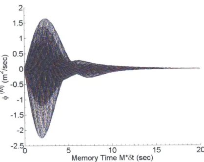
3.5.1 Memory Time Convergence . . . . 92

3.5.2 Size of Time Step Convergence . . . . 96

3.5.3 Mesh Convergence for FIT . . . . 97

3.6 Mesh Convergence between FIT and WAMIT on 2nd order solutions 98 3.7 Numerical Solutions from FIT . . . . 100

3.7.1 MIT/NREL TLP r=9m, T=47.89m . . . . 102

3.7.2 r=3m, T=43.2m . . . . 112

3.7.3 r=1.75m, T=30m . . . . 122

3.8 Comparison between Small Ka with FIT full expression . . . . 132

3.8.1 1st + 2nd Order Surge Force Comparison . . . . 133

3.8.2 Free-Surface Surge Force Comparison . . . . 139

4 Discussion and Future Work 147

Appendices 153

A Free-surface impulse force in Surge 155

B Free-surface impulse force in Heave 167

C Free-surface impulse force in Pitch 179

List of Figures

2-1 Free-surface interaction with floating body . . . . 24

3-1 3-2 3-3 3-4 3-5 3-6 3-7 3-8 3-9 3-10 3-11 3-12 3-13 3-14 3-15 3-16 3-17 Surfaces and vectors included in numerical analysis using FIT . . . . Top view of a cylindrical body and numerical panel elements surround-ing the body surface (Simplified in terms of the number of panel elements) Body mesh with 720 panels for MIT/NREL TLP, r=9m, T=47.89m Body mesh with 1440 panels for MIT/NREL TLP, r=9m, T=47.89m Body mesh with 2400 panels for MIT/NREL TLP, r=9m, T=47.89m Body mesh with 936 panels, r=3m, T=43.2m Body mesh with 684 panels, r=1.75m, T=30m A Quadrilateral uniform-strength source element . Wave spectral density of the JONSWAP seastate Phase of the JONSWAP irregular wave . . . . Wave elevation of the JONSWAP seastate . . . . Surge 1st order .... ... Surge 1st order PSD . . . . Heave 1st order . . . . Heave 1st order PSD . . . . Pitch 1st order . . . . Pitch 1st order PSD . . . . 67 68 70 71 72 . . . . 73 . . . . 74 . . . . 75 . . . . 78 . . . . 78 . . . . 79 .. ... 81 . . . . 81 . . . . 82 . . . . 82 . . . . 83 . . . . 83

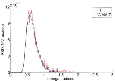
3-19 PSD comparison of total surge force between FIT and WAMIT, r=9m,

T = 47.89m . . . . 86 3-20 Close up PSD comparison of total surge force between FIT and WAMIT,

r=9m, T=47.89m . . . . 86 3-21 1st order surge hydrodynamic force from FIT and WAMIT, r=9m,

T= 47.89m . . . . 87 3-22 PSD comparison of 1st order surge force between FIT and WAMIT,

r=9m, T=47.89m . . . . 88 3-23 2nd order surge quadratic hydrodynamic force from FIT and WAMIT,

r=9m, T=47.89m . . . . 89

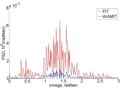
3-24 PSD comparison of 2nd order surge force between FIT and WAMIT,

r=9m, T=47.89m . . . . 90 3-25 Close up PSD comparison of 2nd order surge force between FIT and

WAMIT, r=9m, T=47.89m . . . . 90 3-26 Convergence study for memory time length t = 0 to 100s . . . . 92 3-27 Convergence study for memory time length t = 400 to 500s . . . . 92 3-28 Contribution of memory effects from each time step on Memory

func-tion, (z= 0) . . . . 93 3-29 Contribution of memory effects from each time step on derivative of

Memory function, (z=0) . . . . 93 3-30 Contribution of memory effects from each time step on Memory

func-tion, (z=1/2draft) . . . . 94

3-31 Contribution of memory effects from each time step on derivative of

Memory function, (z=1/2draft) . . . . 94

3-32 Contribution of memory effects from each time step on Memory

func-tion, (z= draft) . . . . 95

3-33 Contribution of memory effects from each time step on derivative of

3-36 Convergence study for mesh density t = 0 to loos . . . . 97

3-37 Convergence study for mesh density t = 400 to 500s . . . . 97

3-38 Mesh convergence for FIT . . . . ... . . . . 99

3-39 Mesh convergence for WAMIT . . . . 99

3-40 Wave spectral density of the OC5 seastate . . . . 101

3-41 Phase of the irregular wave in OC5 . . . . 101

3-42 Surge hydrodynamic force from FIT, r=9m, T=47.89m . . . . 104

3-43 PSD comparison between total, 1st and 2nd order surge force from FIT, r=9m, T=47.89m . . . . 105

3-44 Close up of PSD comparison between total, 1st and 2nd order surge force from FIT, r=9m, T-47.89m . . . . 105

3-45 1st order surge hydrodynamic force components from FIT, r=9m, T=47.89m 106 3-46 PSD comparison of 1st order surge hydrodynamic force components from FIT, r=9m, T=47.89m . . . . 107

3-47 2nd order surge hydrodynamic force components from FIT, r=9m, T=47.89m . . . . 108

3-48 PSD comparison of 2nd order surge hydrodynamic force components from FIT, r=9m, T=47.89m . . . . 109

3-49 2nd order surge free-surface impulse force components from FIT, r=9m, T=47.89m . . . . 110

3-50 PSD comparison of 2nd order surge free-surface impulse force compo-nents from r=9m, T=47.89m . . . .111

3-51 Surge hydrodynamic force from FIT, r=3m, T=43.2m . . . . 114

3-52 PSD comparison between total, 1st and 2nd order surge force from FIT, r=3m, T=43.2m . . . . 115

3-53 Close up of PSD comparison between total, 1st and 2nd order surge force from FIT, r=3m, T=43.2m . . . . 115

3-55 PSD comparison of 1st order surge hydrodynamic force components

from FIT, r=3m, T=43.2m . . . . 117 3-56 2nd order surge hydrodynamic force components from FIT, r=3m,

T = 43.2m . . . . 118 3-57 PSD comparison of 2nd order surge hydrodynamic force components

from FIT, r=3m, T=43.2m . . . . 119 3-58 2nd order surge free-surface impulse force components from FIT, r=3m,

T = 43.2m . . . . 120

3-59 PSD comparison of 2nd order surge free-surface impulse force

compo-nents from r=3m, T=43.2m . . . . 121

3-60 Surge hydrodynamic force from FIT, r=1.75m, T=30m . . . . 124

3-61 PSD comparison between total, 1st and 2nd order surge force from

FIT, r=z1.75m, T=30m . . . . 125 3-62 Close up of PSD comparison between total, 1st and 2nd order surge

force from FIT, r=1.75m, T=30m . . . . 125 3-63 1st order surge hydrodynamic force components from FIT, r=1.75m,

T = 30m . . . . 126

3-64 PSD comparison of 1st order surge hydrodynamic force components from FIT, r=1.75m, T=30m . . . . 127

3-65 2nd order surge hydrodynamic force components from FIT, r=1.75m,

T = 30m . . . . 128 3-66 PSD comparison of 2nd order surge hydrodynamic force components

from r=1.75m, T=30m . . . . 129 3-67 2nd order surge free-surface impulse force components from FIT, r=1.75m,

T = 30m . . . . 130

3-68 PSD comparison of 2nd order surge free-surface impulse force

3-70 PSD comparison between FIT full expression and small Ka approx. for

total surge hydrodynamic force, r=9m, T=47.89m . . . . 135 3-71 Close up of PSD comparison between FIT full expression and small Ka

approx. for total surge hydrodynamic force, r=9m, T=47.89m . . . . 135 3-72 Total surge hydrodynamic force between FIT full expression and small

Ka approx., r=3m, T=43.2m . . . . 136 3-73 PSD comparison between FIT full expression and small Ka approx. for

total surge hydrodynamic force, r=3m, T=43.2m . . . . 137

3-74 Close up of PSD comparison between FIT full expression and small Ka approx. for total surge hydrodynamic force, r=3m, T=43.2m . . . . . 137 3-75 Total surge hydrodynamic force between FIT full expression and small

Ka approx., r=1.75m, T=30m . . . . 138 3-76 PSD comparison between FIT full expression and small Ka approx. for

total surge hydrodynamic force, r=1.75m, T=30m . . . . 139 3-77 Free-surface surge hydrodynamic force between FIT full expression and

small Ka approx., r=9m, T=47.89m . . . . 140

3-78 PSD comparison between FIT full expression and small Ka approx. for

free-surface surge hydrodynamic force, r=9m, T=47.89m . . . . 141

3-79 Free-surface surge hydrodynamic force between FIT full expression and

small Ka approx., r=3m, T=43.2m . . . . 142

3-80 PSD comparison between FIT full expression and small Ka approx. for

free-surface surge hydrodynamic force, r=3m, T=43.2m . . . . 143

3-81 Free-surface surge hydrodynamic force between FIT full expression and

small Ka approx., r=1.75m, T=30m . . . . 144

3-82 PSD comparison between FIT full expression and small Ka approx. for

Chapter 1

Introduction

The energy industry continues to make new strides in constructing and deploying offshore wind turbines with the goal to expand modern society's energy portfolio and provide clean energy for today's ever growing economy. Offshore wind shows great potential as one of the future's prominent energy source due to a variety of reasons. For one, wind is inexhaustible and environmental friendly. The horizontal-axis wind turbine is a mature technology, which allows industries to harvest wind energy at utility scale at low cost. The logistics of the offshore environment favor large multi-megawatt turbines in the 6- to 10-MW range for efficient energy production. These turbines can be easily assembled, transported to, and installed at the offshore wind power plant site. The support structure of offshore wind turbines can be either a bottom-mounted structure in shallow waters or a floating platform if the water is deeper than about 50 m. With much of the worldwide energy demand located at coastal regions, it is imperative to utilize the vast wind resources in the offshore en-vironment.

Fortunately, there exists a vast wind resource potential in deeper water in the

USA, China, Norway, Japan and many other countries ([8], [101, [211). In recent years, the offshore wind industry continues to experiment with different designs of

energy production, wave loads exerted on these floaters by ambient sea states over the life of an offshore wind turbine must be properly modeled and predicted to ensure the structure to be safe and cost-effective.

The wave-body problem

The wave-body interaction problem of an offshore floating structure can be sum-marized as follow. In most seastates, linear wave theory captures most of the leading order aspects of hydrodynamic wave loads on offshore structures. This was theorized

by St. Denis and Pierson

161

as an offshore structure's response to a random sea can be estimated by superposing the response to each wave frequency component in the wave spectrum. This allows a reliability-index-based design method for a given sea spectrum to capture most of the leading order effects in a mild sea condition. There-fore, to avoid possible large load responses, offshore floating wind turbines platforms are often designed to have their natural frequencies to be higher or lower than the dominant ocean wave frequencies.

In extreme and severe sea states or large-amplitude body motions, nonlinear ef-fects are of greater importance and interest in addition to the linear efef-fects. Examples of nonlinear effects include nonlinear hydrostatic load by large-amplitude wave eleva-tions, nonlinear Froude-Krylov force and ringing load by steep large-amplitude waves, and nonlinear wave force by large-amplitude body motions. Large amplitude waves causes extreme wave loads which requires more load bearing capability. When en-countering steep waves, ringing loads may occur and excite the floating structure which leads to potential system failure due to fatigue of the tower (171,

1291).

Among the nonlinear effects, nonlinear hydrostatic force and nonlinear Froude-Krylov and disturbance forces are of greatest concern because they govern limits of the state of loads on tethers and anchors. For certain offshore wind turbine floater design such as the Tension-Leg Platforms (TLP), the nonlinear extreme wave loads may lead to tether overload and tether slack which are undesirable for the foundation design.

an offshore floating structure for wind turbines, as the energy of these nonlinear

ef-fects can reside about the natural frequency of the structure, typically around 1.7-1.8

rad/sec, causing failure of the structure both in the short term and in the long run.

This require an efficient and accurate method for analysis of nonlinear wave loads

on floating structures for their safe and cost-effective design, making it the primary

objective of this work.

Modeling Hydrodynamic Loads

There had been significant advancement in hydrodynamics/wave-body interaction

theory in recent years. The scientific community together with the offshore industries

had come a long way since Froude

[9]

and Krylov [16] first established a theoretical

approach to the hydrodynamic analysis of a floating body's motion.

Currently, the evaluation of the wave loads on offshore platforms is typically

car-ried out either by Morison's equation or by frequency-domain panel methods with

appropriate time-domain transforms for transient analysis. Morison's equation is a

strip theory- based time-domain method for slender structures first theorized by

Mori-son, O'Brien, Johnson and Schaaf

[201.

The method accounts for fluid inertia, added

mass, and viscous effects by selecting appropriate added mass and drag coefficients.

Viscous effects can also be accounted for by equipping appropriate drag and inertia

coefficients derived from experiments.

For large-volume platforms, frequency domain boundary element method based

on the potential flow theory has recently become one of the most popular tools

be-cause of its efficiency and reliability. The first application of BEM was pioneered

by Hess and Smith [11] and later adapted in wave-body problems by Newman and

other scholars

([31,

[231,

[24J). This method is primarily based on linear theory and

model linear and nonlinear potential-flow effects by solving first- and second-order

has resulted in several useful computational methods, an example being the

commer-cial code WAMIT, started here at the MIT Ocean Engineering Department [18].

Previous studies have carried out simulations for floating wind turbines using

Morison's equation and frequency-domain methods. Investigators carried out

com-putations of the loads and responses of TLP floating wind turbines and documented

them in ([2],

[32],

[34]). Simulations for the Hywind Spar floating wind turbine

struc-ture based on Morison's equation were reported by [25]. For the International Energy

Agency Offshore Code Comparison Collaboration (IEA OC3) Spar, simulations were

reported by

113].

For the semisubmersible WindFloat structure, simulations were

presented by [28]. In [26], simulations for the IEA OC3 Continued (OC4)

semisub-mersible were documented. The conclusions from the simulations reported in these

and other studies are summarized here. There is good agreement between

meth-ods predicting the linear potential-flow loads from Morison's equation or

frequency-domain methods. The accuracy of Morison's method deteriorates as the wavelength

of the ambient wave decreases and becomes comparable to the diameter of a

cylindri-cal floater. The agreement between various methods is less satisfactory for predicting

the nonlinear low- and high-frequency loads and responses partly because the

un-derlying modeling assumptions differ and partly because the accurate computation

of the sum- and difference-frequency QTFs is a complex and time-consuming task.

Additional limitation of a frequency domain analysis based on the linear wave and

linear dynamics theory is that the amplitudes of ambient wave and body motions

have to be small compared to the ambient wavelength. The linearity assumptions on

the wave and motion amplitudes hamstrings investigations of crucial hydrodynamic

interactions between waves and bodies in severe seas. Excessive computational cost

involved with the complexity of fluid and body interaction also limits the

develop-ment of the three-dimensional fully nonlinear numerical schemes. An alternative to

the methods discussed above are time-domain potential flow methods for the

com-putation of second order loads. The nonlinear time-domain solvers have yet to reach

The Fluid-Impulse Method

The goal of this work is to explore and develop a new versatile, accurate and

ef-ficient time-domain potential flow method for the treatment of nonlinear wave-body

interaction in irregular waves in the time-domain. The new method, the Fluid-Impulse

Theory (FIT), is based on new expressions for nonlinear hydrostatics, Froude-Krylov,

and radiation and diffraction loads derived by Sclavounos [30]. Further description of

the theory is presented in the theory section of this thesis.

The time-domain fluid-impulse method bridges the gap between long-wavelength

approximations in the time-domain Morison's equation and frequency domain

meth-ods. It can be used for both slender and large volume offshore structures and allows

for the modeling of higher-order transient nonlinear effects in the vicinity of the

wa-terline. In addition, the fluid impulse method allows the evaluation of second-order

and higher-order nonlinear effects via compact force expressions that circumvent the

discretization of the free surface by taking advantage of the analytical structure of

the time-domain Green function.

Overview

The rest of this thesis is organized as follows. Chapter 2 presents theoretical

for-mulations: the boundary value problem for a hydrodynamic wave-body interaction,

the force and moment components in FIT formulation, the solution of the disturbance

potential by solving a set of integral equation using the transient free-surface

Green-function method and the source formulation, and detailed derivation on solving the

free-surface impulse component in FIT. Chapter 3 presents numerical algorithms and

simulation results: the wave loads obtained by FIT formulation using the Perturbation

Theory, the treatment of surfaces and generation of body mesh, the representation of

surfaces with constant-strength source elements, verification and comparison studies

between FIT and WAMIT, several test cases obtained by FIT for buoy of different

Chapter 2

Theory

This chapter discuss the theory behind the computation of hydrodynamic loads using the Fluid-Impulse Theory (FIT). The goal of FIT is to provide a formulation for the computation of nonlinear hydrodynamics loads in the time-domain for body of any size in the ocean. This chapter starts by summarizing the formulation of FIT and discusses the different force and moment components in the formulation. In the formulation, as the ambient wave is assumed to be known, the only unknown is the Radiation and Diffraction (RD) potential, or the disturbance potential. The solution of the disturbance potential is obtained by solving a set of integral equations using the transient Green function and the source formulation. The transient Green function and the source formulation are described theoretically and numerically in their respective subsections. A theoretical framework on expressing the completely nonlinear term, the free-surface impulse force and moment components in surge, heave and pitch, with respect to known body surfaces is then presented for the efficient application of FIT. This allows FIT to be applied efficiently without the need of discretizing the ambient wave free-surface, while accounting for the nonlinear load contributions from the ambient irregular seastate. Finally, a summary on a simplified FIT formulation using the small Ka approximation for surge wave loads on cylinders is presented at the end of this chapter.

2.1

Fluid-Impulse Theory Formulation

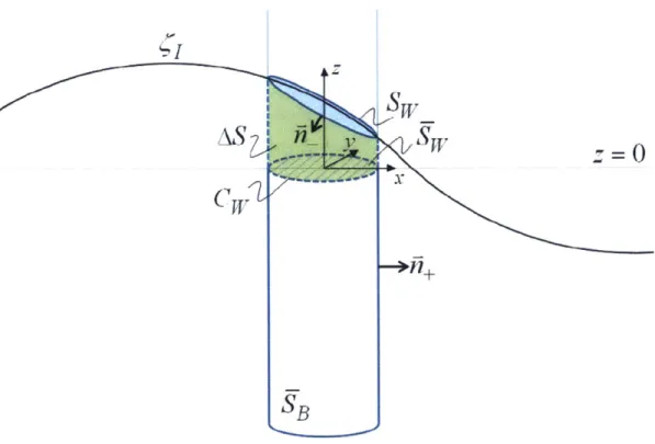
Fig. 2-1 illustrates a platform floating on a free surface interacting with a nonlinear ambient wave assumed to be irregular. The reference coordinate system (X, Y, Z)

is fixed in space with its origin located on the calm water surface with the positive Z-axis pointing upward. The free-surface elevation resulting from the ambient wave is denoted by the solid line. The dashed line defines a horizontal plane intersecting the Z-axis at the local elevation of the ambient wave profile. The acceleration of gravity is g and the water density is p.

The ambient wave velocity potential is denoted by 0b(X, Y, Z, t) and assumed to

be irregular and traveling in deep water:

(polychromatic)

#j(x,

y, z, t)=R igiyezivjxcos jiivysinj+iwt+ix1

J

(2.1)

where vj = W]/g.

And the disturbance radiation and diffraction potentials are denoted by

#(X,

Y, Z, t). 1JOUL potenitials are suUject u Ut LaplaCe

tequation

in bite HuiM doinain as

02 + 02 + Z0. (2.2)

On the instantaneous position of the body boundary SB(t), the normal velocity of the radiation potential is equal to the normal velocity of the body boundary U, because of its oscillatory motions

UTI on SB- (2-3)

On

In the diffraction problem, the diffraction potential offsets the ambient wave nor-mal velocity on SB (t)

after denoted by the same symbol, with the body boundary conditions from (2.3) and (2.4) applying for each potential, respectively.

z =

(X

.Y,.

_t)

_z

_L

_-(t

(S

(t)

The Fluid Impulse Theory (FIT) derived by [301 is capable of accounting the fully nonlinear free-surface by taking applying a fully nonlinear dynamic and kinematic free-surface condition in the boundary value problem. As this work focuses on study-ing the leadstudy-ing order nonlinear effects of a wave-body problem, the disturbance RD potential

#

in FIT was linearized about the ambient wave surface S1(t) exterior to the body waterline as

a

2

_o

₀₀

Ot2 + Y aZ = 0, on S1. (2.5)

The conventional definition of the force and moment acting on the body follows from the integration of the hydrodynamic pressure obtained from Bernoulli's equation over the instantaneous body wetted surface

F =

-J

V0 + +4) -V(O1 + 0) + gZj rds

SB _(2.6)

a=- +-2V(Oi + )V(01 +0) +gZ x (X x n ds.

SB

The evaluation of the nonlinear hydrodynamic force and moment given by (2.6) requires the computation of the partial time and space derivatives of the disturbance potential over the instantaneous wetted surface of the body. This computational task requires fine panel meshes that lead to slow convergence in the evaluation of nonlinear forces.

The FIT formulation circumvents the computation of gradients of the disturbance potential by deriving new expressions for the hydrostatic and hydrodynamic forces summarized in the following sections. The total force and moment in (2.6) can be represented as the sum of four components as described in (2.7): 1) nonlinear buoy-ancy force and moment; 2) Froude-Krylov impulse force and moment; 3) radiation and diffraction body impulse force and moment; and 4) radiation and diffraction free-surface impulse force and moment.

These force and moment expresssions are discussed in further details in the following subsections.

2.1.1

Nonlinear Buoyancy Force and Moment

The hydrostatic force and moment acting on the body takes the following form

FH = pgVwk -pg

J

Zds _(2.8)

SB+SW

PH-pg Z(X x n dS (2.9) SB+SW

In (2.8) and (2.9), k is the unit vector pointing in the positive Z-direction and Vw(t) is the volume enclosed by the body wetted surface SB(t) and the nonlinear ambient wave surface interior to the body Sw(t), defined in Fig. 1. The nonlinear hydrostatic force given by (2.8), then, always points upward. In the classical definition of the nonlinear body force obtained by integrating the hydrodynamic pressure from Bernoulli's equation in (2.6), the nonlinear hydrostatic force depends on the shape of the body wetted surface and does not necessarily point upward. (2.8) extends the classical Archimedean buoyancy force in calm water to the unsteady case of nonlin-ear wave body interactions via the introduction of a time-dependent displacement bounded by the body wetted surface and a dynamic water plane area defined by the ambient wave.

2.1.2

Froude-Krylov Impulse Force and Moment

This force and moment takes the following form

FF-K =-P

J

ilds (2.10)

The surface integrations in (2.10) and (2.11) are carried out over the instantaneous intersection of the body boundary and the ambient wave profile, which is assumed to be known with the unit normal vector pointing inside the body. An additional integration is carried out over the ambient wave free surface interior to the body. An application of Gauss's theorem provides an alternative definition of the Froude-Krylov impulse as the integral of the ambient wave velocity vector over the volume internal to the body wetted surface and its dynamic water plane area. The evaluation of the new Froude-Krylov force and moment requires knowledge of only the velocity potential of the ambient wave over the body boundary and not its partial time derivative or its

spatial gradients.

2.1.3

Radiation and Diffraction Body Impulse Force and

Mo-ment

This force and moment takes the following form

FB P Jpds _(2.12)

SB

IB

~ -~

(X

xn (2.13)

SB

The integrations in (2.12) and (2.13) are carried out over the instantaneous body wetted surface defined by its intersection with the ambient wave profile. Again the evaluation of the forces and moments requires only the RD velocity potentials over the body boundary and not their partial time derivative or spatial gradients.

2.1.4

Radiation and Diffraction Free-Surface Impulse Force

and Moment

The remaining nonlinear free-surface force and moment invovles integrals of the ra-diation and diffraction disturbances over the ambient wave free surface S1(t).

d

_C

FFS - qn'ds - pgk] ds Si Si (2.14) - p f CV#+0) + '(2 ZV( 1+0)

+..

ds

SI SI SI(2.15) d

f

_{1( a} -- pt X X V(#r +0)] + OZ X V(OI + 0)]+. ds S.1

Further derivation of this force and moment is discussed in Section 2.4.

2.1.5

Summary

In summary, the nonlinear hydrodynamic force acting on a body floating in an ambient irregular wave of large amplitude has been derived as the sum of a nonlinear buoyancy force pointing upward and the time derivative of a sequence of impulses. The Froude-Krylov nonlinear impulse involves an integral of the ambient wave velocity potential over the instantaneous body wetted surface and the interior water plane area defined

by the ambient wave elevation. The body RD nonlinear impulse involves an integral

of the RD velocity potentials over the body wetted surface. The free-surface RD nonlinear impulse involves integrals of the RD disturbances over the infinite ambient wave free surface exterior to the body waterline. The forces discussed in this section are based on the assumption that the RD velocity potentials satisfy the linear free-surface condition over the ambient wave free-free-surface profile. Higher-order nonlinear

2.2

Integral Equation for the Disturbance Potential

As discussed in Section 2.1, the ambient wave velocity potential

#

1(X, Y, Z, t) is

as-sumed to be known a priori. To compute the forces and moments presented using FIT, the disturbance potential 0(t) is the only unknown.

The disturbance potential 0(t) satisfies the linearized free-surface condition in (2.5) on the ambient wave surface illustrated in Fig. 1. The horizontal dashed planar surface illustrated in the figure intersects the Z-axis at the ordinate (1(0, 0, t) = (r(t). To take advantage of the analytical properties of the time-domain Green function, the free-surface condition (2.5) is hereafter assumed to be valid on the planar surface

Z = ((t). This assumption is justified by the small slope of steep waves in a sea state. Introduce the new coordinate system centered on the dashed planar surface as follows

x X

y Y (2.16)

z~)= Z -1t

The Laplace equation maintains its original form relative to the new coordinate system. The free-surface condition, satisfied by the disturbance potential relative to

the new coordinates p(x = X, y = Y,z Z - (I(t), t) =

#(X,

Y, Z, t), follows from

these identities

0#(t)

00(t)

OBP(t) Oz

OW(t)

-

V(t)

=

+

=r

- (iM)

at

at

+ z at

at

Oz

(217) a2#(t) 02p(t) 92p (t) t +p - 2 p t (2.t)

at2

-

2(azat-

(t)

a

Z

(

2

Introducing (2.17) in (2.5), the free-surface condition relative to the new coordi-nate system becomes

02 (t) .. W(t) 02 P(t) - 2 p(2

incident wave elevation are of the order of 6 = KA relative to the leading order terms, where A is the characteristic amplitude of the ambient wave and K is the characteristic wave number. Consequently, the free-surface condition relative to the new coordinate system, with relative errors of 0(6), becomes the following:

t

2

_(+g

_=z

_{0, z = 0}

_(2.19)

The body boundary conditions in (2.3) and (2.4) maintain their form because they involve only spatial derivatives. They are enforced on the instantaneous wetted surface of the body defined relative to the new coordinate system.

From the preceding analysis, it follows that the free-surface condition in (2.19) is enforced on the planar z = 0 surface at each time step. Relative to this plane the body wetted surface is more submerged below z = 0 when (I(t) > 0 and less submerged when (1(t) < 0. The vertical coordinate of a point of the body wetted

surface is given by z Z - (I (t), where Z is the vertical coordinate relative to the earth-fixed frame.

The boundary value problem for the disturbance potential becomes a body non-linear time-domain free-surface problem subject to the non-linear free-surface condition. Invoking the time-domain Green function, a time-convolution integral equation can

be derived for the disturbance potential along the lines of

[331,

[35J. The disturbance

velocity potential is represented by a distribution of sources over the instantaneous wetted surface of the body, as follows

($,

t)

=

Jds

o , t)(

,-1)

SB(t)

+ s(2.20)

+

J

dTr

JJ

ds

U($,T) H(Y~, t - T)

as follows

n

V(,) -s-( x On iV sa t)( 417 r r' S -B

M(2

_{.2 1 )}

+ jdT

ds

o(,T)Hr(,

,t T)1 0 SB(T)

The left-hand side of (2.21) is a known normal velocity on the body wetted surface for the RD problems via (2.3) and (2.4), respectively.

Invoking the following notation,

x (x, y, z)

(2.22)

r [(x - )2 + (y - 77)2 + (z - ()211/2

r [(x -- )2 + (y - q)2 + (z + ()2]1/2

the time-domain Green function is defined as follows

G (0) (z,5)=

HT(s, t) - -, dk /gek(z+) sin[V/gkt]Jo(kR) (2.23)

0

R = [(x - )2 + (y - rq)2]1/2

The integral equation in (2.20) through (2.23) is solved by discretizing the instan-taneous body wetted surface with planar panels and advancing the time-convolution integral ahead in time starting at t = 0.

The velocity potential of the incident wave W(', t) is based on the standard repre-sentation of an irregular wave train in a sea state. The solution of the integral equation in (2.21) provides the disturbance velocity potential over the instantaneous position

and body forces. This is carried out by first integrating the velocity potentials over the body wetted surface and then taking the time derivative of the resulting time-dependent integral. The evaluation of the partial time derivative and spatial gradients of the ambient and disturbance potentials is circumvented. The free-surface impulse force in Eqs. (2.14) and (2.15) is evaluated in Section 2.4.

2.3

The Transient Wave Part of the Green Function

The transient wave part of the Green function (2.23) described by Wehausen & Laitone [35] can be evaluated in several different ways. Its formulation is listed again below as:

00

HT(?, ,t - ) - dk VfgkekZ sin[Vgk(t - T)]Jo(kR)

0

r [(x - )2 + (y - 1)2 + (z - ()211/2

' [(x - )2 + (y - q)2 + (z + ()2]1/2 (2.24)

Z z

+

()

R

=[(X - )2 + (y 71)2]1/2

In this work, the wave part of the Green Function was computed numerically by two methods: 1) by solving the ordinary differential equation as described by Clement

[5]; or 2) by the methods described by Newman [22].

2.3.1

Clement

As derived by Clement [5], the wave part of the Green function HT(, f, t - T) stated above can be evaluated by solving an ordinary differential equation. Rewriting Hr(X,,t T) as:

CO

Hr(X, , t - T) = F(r, Z, t -Tr) = - f dk V/k-ekZ sin[Vdh(t - T)]Jo(kR)

0

(2.25)

Let r1 r2

+

Z2, with a change of variable (krl -+ A), Jami [12] showed that

the memory part of the Green function can be expressed as a function of two variables

with

F(t, T) fdA ve-A/ sin[VXT] Jo(A /1 - p2) (2.27)

0

where = -Z/ri and T= Fg(t - T)/f/rj.

F satisfies the following fourth-order differential equation:

+ IT + (2 + 41) + 4 + F = 0. (2.28)

with the initial conditions

P(2k)(, 0) = 0, p(2k+1)(p, _{0) =} (-1)k(k + 1)!Pk+((p); k = 0, 1, ... (2.29)

where P(k) denotes the kt-order differentiation of F with respect to T.

Further study by Chuang et. al [41 stated that a Taylor series expansion method can be applied to solve the differential equation (2.28) with low computational cost. Eq.

(2.28) is rewritten as:

K

()+TK( + (T2

+Ap

K

+ BTK(P

+ CKF

0

7(9 (2.30)

7

9

where A=4; B- , C= for KF

-Introducing the expression:

Based on the work of Chuang et. al [4], the coefficients a., can be obtained using the closed form solution:

1

a4 _24K1- (6K3a3

+

2K2a2 + K8a1 + Kgao)

1

1

a,,+4 =:' 1

(yn+3an+3

+ yn+2an.+2 + yn+ian+1 + ynan), for n 1, 2, 3,...

where Yn+4 = K1(n _{+ 4)(n + 3)(n + 2)(n + 1) (2.32)} Yn+3 = K3(n + 3)(n + 2)(n + 1) Yn+2 = K2(n + 2)(n + 1)n + K6((n + 2)(n + 1) Yn+1 = 5(n + 1)7 + K8(n + 1) yn = K4n(n - 1)

+

K-n + r'.

Once these coefficients are obtained, P can be computed and therefore the wave part of the Green function can be evaluated very efficiently from the computational perspective.

To compute the derivate of F for the evaluation of the derivative of the Green function,

by the extension of the Taylor series method presented by Chuang et. al [4], the

differential equation can be solved by taking (2.30) with new constants:

11 21

A=6; B--; C=- for KF -K. (2.33)

2.3.2

Newman

Another way of evaluating the transient wave part of the Green function is described in Newman [221. Transforming (2.24) using the spherical coordinates (ri, 0), with the angle 6 measured from the negative vertical axis.

Nondimensionalize the phusical parameters again with repect to g and ri:

0

= arccos(p) = arccos(-Z/ri), T =f -

(2.34)

The transient wave part becomes

HTF, f, t -F) =

( -

girT {(0,T)}

where

(2.35) 00

F

= -4i w2eiw-wT2cos Jo (w2 sin 0)dw; w -

k1/2

0

The computational domain is now (0 < T < oc, 0 < 0 < 7r/2).

For large value of T, asympototic expansion was derived in [22]. The function can now be decomposed into two parts:

S=

f

+ f1 + f2 (2.36)

The first part of the integral, integrating P in (2.35) up to iT/2, can be expanded using Watson's Lemma, and can be expressed as:

f

-4

(2n+

2_{)! T-2n-3Pn(COS}

0) (2.37)

The second part of the integral, fi was proven to be exponentially small for all values of

0,

and through a series of transformation outlined in [22], f2 can be rewritten into: f 2 s-4

i

2 si n9

24

(2.38)

si j n YdnmW2-2m-2n.-imO sin) m M=O

where doo = 1, dom = 0 for m > 0, and for n >

1

dnm = Cn (2m + 2n - 2)! (2n - 2)!22 mm!

and

[Cf(n +

]2 Un _7r2nn!

(2.39)

(2.40)

2.4

Free-Surface Impulse Force

Linearing the equations (2.14) and (2.15) above the free-surface using linear FSC

(2.5):

1 &q#

on S1. (2.41)

g at

Keeping terms up to leading order quadratic effects, the free-surface impulse force and moment expressions become:

d 8# d f10# FFJ=+ds + pJ -+V(oi+ O)ds (2.42) Si S1 SI MFS =-P + Xx -) ds+pJ (X x kPds S_{1 d 100 S} (2.43) P_ g 8t$x V(OI+4) ds SI

The unit normal vector to the ambient wave free surface may be expressed in terms of the gradients of the free-surface elevation. Denoting by 6 the order of magnitude of the ambient wave slope obtains the following, with errors quadratic in the wave slope

V (Z - ((1( XY1t 0) -iC1, - JC1, + k

|V(Z - (1(XY,t) 1 + _(2.44)

= (-iC1x - Jj1, + k)[1 + 0(62)]

Invoking again the linear FSC (2.41), and keeping the leading order unit normal vector:

(

1 &2 q, (2.45)

Substituting (2.45) in (2.42) and (2.43), the force in the surge and heave are respectively:

PFFSl J

- 2+1

(0+)ds

(2.46)

FyS1 gdl j aXatds g dt a t OX(+4 s2.6

SI Si

d ( p pd #

FFS,3 = -P- j ds + p Jds + I

K-

Y

(

H+

ds (2.47)

SI SI SI

By moving the derivative of the first term of the force expression inside of the

integral and keeping terms to the leading order, the first term of the heave force expression can be shown to cancel with the second term, thus leaving only the last term of the force expression to be computed:

-. p d (0 ap

FFS,3

g dt

__t

Z( $

ds

(2.48)

In the pitch direction, following (2.44), the cross product between the position vector and the unit normal vector and the gradient of velocity potentials X x n',

X x k, X x VW1 and X x VW in the pitch direction are respectively:

Z

) (z(} - x) 0(62)

( X V k ) - (2.49)

Xx r =Xo x8Z1

xV) = z -x O

The pitch moment is thus:

d 00 fo

A'IFS,5 ~ -P- J (z( - x ds

+

p (-xds

For small wave steepness, the pitch moment is evaluated on z = 0 , the remainder of the first and second integral cancels and the moment expression is reduced to:

p

d

0p 0p1

490

AFS,_{5 = t}

J

_{X +} ds (2.51)

S1

The fluid-impulse force and moment in (2.14) and (2.15) involves quadratic and cubic products of the incident and disturbance potentials. This section described the transformation of the expressions using the lienar FSC as well as assuming small ambient wave steepness. To further simplifed the expressions, the ambient wave free-surface can be linearized locally at the ambient wave waterplane at the body. Thus all integral over the ambient free-surface are evaluated at z = 0 with z = Z - (I(t).

The following subsections discuss the free-surface impulse force futher based on these assumptions.

Before starting the derivations of the free-surface impulse force and moment in the surge, heave and pitch direction, the definitions of the incident wave velocity po-tential and the disturbance popo-tential are revisited here:

'pi in irregular waves in deep water, according to (2.1), is:

(polychromatic) 'p (x, y, z, t) = evjz-ijx cos 3j -vjysin j+iwjt+ixj

V3 = W(2g.

And the disturbance velocity potential is: y(X, y, z, t) = P(0)(x Y, z, t)

+

p(AI)(x, y, z, t)

IP(X

y, ^z, t) J (0 dsco-(, t)

(I) (X, y,

/,

=

Jt)

(1 HT,7,t-T) = -where Jo(kjR)= j

J

dkj gkjek(z+) sin[ 0 e ikRcosOidO; Ngk(t -

T)]Jo(kjR)

R

= [(x - ( )2 + (y - 77)211/2

and x - = R cos'; y - r = Rsin @

Again with small wave steepness approximation, p(0_{)(x, y, 0, t) = 0, t > 0 by}

definition. Thus 9 (O)(x, y 0,t) = 0, t > 0.

V(x, y, 0,t) = (A)(x y, 0, t)

H,(Y, t - T) = d

2-/To

I

dr

<u(-T)(-,

H(,, t - T)

kj 1gekj (sin[ gk(t - T)]Jo(kjR)

The analysis proceeds by evaluating the free-surface impulse force on z = 0; The function H, can be rewritten as:

let uj = k cos -}j; = kj -j sin j;

7r 00

thus dudvj = kdkjd-y

(2.55)

J

dk gkjekj sin[ g k(t - T)1CikincoCs0i 0 dT

f

d((,

r)HT(,

, t - T) 00 (2.53) (2.54) -1 H,(z ft - _{7r E j d} i -.7r

H, is then:

HT(, , t - r) = - dujdv3 g eki sin[. gk(t - T)]eiui(x-s)+iV(y-r7)

(2.57)

2.4.1

Free-surface impulse force in Surge

The X-direction free-surface impulse force (2.46) can be rewritten into two terms: an

ID term which involves cross-products of the incident and disturbance potentials, and

a DD term which involves a quadratic product of the disturbance potential:

FFS,1 FS,1-ID + FS,1-DD -. 1 p d

J

j

- OPo d FFS,1 ID ds g d= Oxot &t Ox FFS,1-DD

N--f(&'oa~

s

z=O (2.58)

For the first term, the ID component in (2.58), the ambient wave free-surface SI(t) can be split into the difference between the infinte free-surface S,,(t) and the ambient wave surface inside of the body Sw(t):

__#p d

(f

2 o1 ,oapi"\ ds JFS,1-ID - at Ox

J

So. SW d p [O2<p W 2p(t W__ OW __ dt g J xot x ) Ot OxOt It Ox Sw S" (2.59)

The impulses for this force expression can then be identified to be an integral over

Sw(t) and another over So,(t), which is equivalent to a 2D infinite integral over the

x- and y-direction: FFS,1-ID ciFS,1-ID IFS,i-IDSw - (2 .0s 9 g11 axot at ax _(2.60) IFS,1-IDS = -x g_0 axot at Ox

This utilizes the property that both the incident wave and both components of the disturbance potential and their time partial derivatives are continuous across the body waterline and over the z = 0 plane. The first impulse over the finite surface

Sw (t) can be evaluated numerically directly by quadrature with information about all

components inside the integral obtained with the expression of pI(t) and V(t) listed in (2.52) through (2.57) and by taking their spatial and time derivatives. Note that the value and the time derivative of the impulsive part of the disturbance potential

p(0)(t) are zero onz=0as discussed before. Therefore only the memory part of the

disturbance potential yp(^)(t) contributes to the surface integral over Sw(t).

The second integral in (2.60) is over the entire z = 0 plane and its computation by

numerical means would be time consuming if computed directly. An efficient way of computing this integral in the time-domain can be derived by taking advantage of the Green function and its analytical representation listed in (2.54) and (2.57). Again, the value and the time derivative of the impulsive part of the disturbance potential

(0) (t) are zero on z = 0 and only the memory part of the disturbance potential (P(AI) (t) contributes to the surface integral.

Substituting (2.52) through (2.57) in the second integral in (2.60) and invoking

the definitions of the delta functions:

dxeix(uiuv cos 3i) = 27r6(uj - vj cos3j)

(2.61)

dyeiy("-i -jsin fli) = 27r6(vj -vj sin O3)

-00

an

dxdyeiujx

a(U oS ivjx s i+ivjy-ivjy sin nO :

j

-

= 4rel -i

and the relation:

t

+ I

F()dT = F(t)

dt

0

The final expression for FFs,1-1D(t) can be expressed as:

FFS,1-ID p

pd

P 2 I - gdt

OxLa~t

-SW where K(vj, /3 , t) 0 0 _{&0 i] ds} JSB

<or(

4

{

A wj

cos

3j

eitixi

K(vj,

3i , t)}

- p!R

For detailed steps on the mathematical derivations please see Appendix A.

-00

I

-00 - vu sin3j) (2.62) (2.63) (2.64)

For the second term, the DD component in (2.58) contains an integration of a quadratic product of the disturbance potential of the z = 0 plane outside the body waterline. The time derivatives maybe transferred under the integral sign by utilizing the Reynolds transport theorem:

pd

f

V ( <p0p\ F S,1-DD ~~-- x g d t Z = t O X ( . 5 pf d - _{"pOPds + -}p 09 096 dl

Un

g dt Ot Ox 9 "Ot OX =O _Cw

The last integral over the body waterline in (2.65) involves the normal oscillatory velocity of the body which is of the same order as the disturbance potential, therefore it is of cubic order and is omitted. Note that for a ship advancing with a significant forward speed, this integral is of the same order as the first term and should be considered when computing free-surface impulse force.

Performing a formal differentiation of the terms under the integral sign in (2.65) gives:

~

(2.66)

at at Ox) OtP

Ox

ox aUt

Upon substitution in (2.65) the DD component of the free-surface impulse force can be expressed as:

p fT O2<p p pf0 2 p0p p f OW 2

FFS,1-DD _{x- 1x didyt llat} 2

-ds+-gj 1 O x Ox 2g \akt /

-oo -o Sw Cw

The Stokes' theorem was invoked over the z = 0 plane in (2.67) to reduce the

integral of the x-derivative in the last term of (2.66) to an integral over the body waterline. The integral of the first term in the right hand side of (2.66) over the body interior waterplane area was also added and subtracted. The second and third term in (2.67) can be evaluated directly using the definition (2.54) of the disturbance potential over the according surface and waterline.

For the evaluation of the infinite integral in (2.67), invoke the free surface condition

(2.19) satisfied by the total disturbance potential and introduce the velocity potential

decomposition into the instantaneous and memory components:

_2 P ₀

(M)

0

(M)

OP(O) OjP(M)

= -g - Z-g z=0 (2.68)

0t2 Ox x Oz Oz Ox Oz Ox

(2.68) was obtained by utilizing the property that the value and the x-derivative

of the velocity potential component yp(O) is zero on the z=0 plane at all times. The infinite integral in (2.67) is therefore:

0 0 00 (A0l

p _]dx f _dy---- 2 O<r _{(-g) dx dy.}

(

) 0 tpNI) ₊

a<po)

v0p P

(2.69)

g jOt 2 x g

J

O x OZ O x

-00 -00 -00 -0

The memory component of the disturbance velocity potential is harmonic in the lower half space for z<0 and it vanishes at infinity. Therefore, by utilizing the familiar vector identity over a closed surface bounded by the z = 0 plane and a semi-spherical

surface at infinity over which the integrand vanishes:

00 00

[d~d(

~(~f)

(AI) A-1 ) .(M))

dx _

dy ( Vp 2 p -p 0 (2.70)

-0 -00

The unit vector I' points in the vertical direction. The x-component of (2.70) is:

dx dy = 0 (2.71)

Combining (2.69) and (2.71) gives:

p 0 2 (0,OW(0) O V(A)

- dx

J

dy =t2 -p dx dy- (2.72)