HAL Id: hal-00288529
https://hal.archives-ouvertes.fr/hal-00288529
Submitted on 17 Jun 2008
HAL is a multi-disciplinary open access
archive for the deposit and dissemination of
sci-entific research documents, whether they are
pub-lished or not. The documents may come from
teaching and research institutions in France or
L’archive ouverte pluridisciplinaire HAL, est
destinée au dépôt et à la diffusion de documents
scientifiques de niveau recherche, publiés ou non,
émanant des établissements d’enseignement et de
recherche français ou étrangers, des laboratoires
Mathematical models and reconstruction methods in
magneto-acoustic imaging
Habib Ammari, Yves Capdeboscq, Hyeonbae Kang, Anastasia Kozhemyak
To cite this version:
Habib Ammari, Yves Capdeboscq, Hyeonbae Kang, Anastasia Kozhemyak. Mathematical models and
reconstruction methods in magneto-acoustic imaging. European Journal of Applied Mathematics,
Cambridge University Press (CUP), 2009, 20 (3), pp.303-317. �10.1017/S0956792509007888�.
�hal-00288529�
Mathematical Models and Reconstruction Methods in
Magneto-Acoustic Imaging
∗
Habib Ammari
†Yves Capdeboscq
‡Hyeonbae Kang
§Anastasia Kozhemyak
¶Abstract
In this paper, we provide the mathematical basis for three different magneto-acoustic imaging approaches (vibration potential tomography, magneto-magneto-acoustic tomog-raphy with magnetic induction, and magneto-acoustic current imaging) and propose new algorithms for solving the inverse problem for each of them.
1
Introduction
In magneto-acoustic imaging, a probe signal such as an acoustic wave or an electric current (or voltage) is applied to a biological tissue placed in a magnetic field. The probe signal produces by the Lorentz force an induced signal that is a function of the local electrical conductivity of the biological tissue [14]. If the probe signal is an acoustic wave, then the induced signal is an electric current and the Lorentz force causes a local current density.
Induced boundary currents (a) or pressure (b) which are proportional to the local elec-trical conductivity can be measured to reconstruct the conductivity distribution with the spatial resolution of the ultrasound. The induced signal is detected and an image of the local electrical conductivity of the specimen is generated based on the detected induced signal. Method (a) is referred as the vibration potential imaging and method (b) as magneto-acoustic tomography with magnetic induction. The vibration potential imaging is also known as the Hall effect imaging.
Method (a) can be applied to body tissue in vivo and to measurements in suspensions and cultured cells. The ultrasound beam ensures the excitation of the desired region of in-terest and the interaction current is collected by means of electrodes. It is a very promising direction of research for improving the electrical impedance tomography (EIT). EIT is an
∗H.A. and Y.C. are partially supported by the ANR project EchoScan (AN-06-Blan-0089), H.K. is
par-tially supported by the grant KOSEF R01-2006-000-10002-0, and H.A. and H.K. are parpar-tially supported by STAR project 190117RD
†Laboratoire Ondes et Acoustique, CNRS & ESPCI, 10 rue Vauquelin, 75231 Paris Cedex 05, France
‡Mathematical Institute 24-29 St Giles’ Oxford OX1 3LB, UK ([email protected]).
§Department of Mathematical Sciences and RIM, Seoul National University, Seoul 151-747, Korea
¶Centre de Math´ematiques Appliqu´ees, CNRS UMR 7641 and Ecole Polytechnique, 91128 Palaiseau
imaging technique focused upon reconstructing the impedance distribution of biological tis-sue using current injection and noninvasive voltage measurements. In EIT, electrical current is injected into the object from electrodes attached to the surface, and the corresponding boundary voltage is measured over the surface of the object in order to reconstruct the impedance distribution within the volume. It is known that this approach for imaging the conductivity distribution produces images with deceivingly poor accuracy and spatial res-olution. The vibration potential imaging relies on innovative measurement techniques that incorporate structural information. Its intrinsic resolution is of order of the size of the focal spot of the ultrasound, and thus it should provide high resolution images.
If an electrically active tissue is placed on a magnetic field then an acoustic wave or tissue displacement is created. This method (c), known as magneto-acoustic current imaging, has been suggested as a method for reconstructing current dipoles and imaging action currents arising from active nerve or muscle fibers by detecting the induced pressure signal.
We refer the reader to [14, 12, 13, 17, 18, 8, 15, 16] for physical basic principles of vibration potential tomography, magneto-acoustic tomography with magnetic induction, and magneto-acoustic current imaging.
In this paper, we provide the mathematical basis for these three different magneto-acoustic imaging approaches and propose new algorithms for solving the inverse problem for each of them.
2
Mathematical Formulations
2.1
Vibration Potential Tomography
We recall that, in mathematical terms, EIT consists in recovering the conductivity map of a 2D or 3D body Ω (of class C1,α, α > 0), from one or several current-to-voltage pairs
measured on the surface of the body. Denoting by γ(x) the unknown conductivity, the voltage potential v solves the conduction problem
∇ · (γ∇v) = 0 in Ω, v = g on ∂Ω. (2.1)
The problem of impedance tomography is the inverse problem of recovering the coefficients γ of the elliptic conduction partial differential equation, knowing one or more current-to-voltage pairs (g,∂ν∂v|∂Ω). Throughout this paper, except in Section 4, we assume that g ∈
C1,α(Ω) and the conductivity γ ∈ C0,α(Ω), and is bounded in Ω above and below by positive
constants. The solution v is then in C1,α(Ω). Further, we suppose that the γ is a known
constant on a neighborhood of the boundary∂Ω and let γ∗ denote γ|∂Ω.
In vibration potential tomography (VPT), ultrasonic waves are focused on regions of small diameter inside a body placed on a static magnetic field. The oscillation of each small region results in frictional forces being applied to the ions, making them move. In the presence of a magnetic field, the ions experience Lorentz force. This gives rise to a localized current density within the medium. The current density is proportional to the local electrical conductivity [14]. In practice, the ultrasounds impact a spherical or ellipsoidal zone, of a few millimeters in diameter. The induced current density should thus be sensitive to conductivity variations at the millimeter scale, which is the precision required for breast cancer diagnostic. The feasibility of this conductivity imaging technique has been demonstrated in [6].
Let z ∈ Ω and D be a small impact zone around the point z. The created current by the Lorentz force density is given by
Jz(x) = cχD(x)γ(x)e, (2.2)
for some constant c and a constant unit vector e both of which are independent of z. Here and throughout this paper, χD denotes the characteristic function of D. With the induced
current Jzthe new voltage potential, denoted by uz, satisfies
∇ · (γ∇uz+ Jz) = 0 in Ω,
uz= g on ∂Ω.
According to (2.2), the induced electrical potential wz := v − uz satisfies the conductivity
equation: ∇ · γ∇wz= c∇ · (χDγe) for x ∈ Ω, wz(x) = 0 for x ∈ ∂Ω. (2.3)
The inverse problem for the vibration potential tomography is to reconstruct the conduc-tivity profile γ from boundary measurements of ∂uz
∂ν |∂Ωor equivalently ∂wz
∂ν |∂Ωfor z ∈ Ω.
Throughout this paper, we assume that γ is constant in D. This assumption is natural since the resolution can not be lower than the characteristic size of the ultrasonic beam. Recall that γ is known in a neighborhood of the boundary ∂Ω.
Let |D| denote the volume of D. Since γ is assumed to be constant in D and |D| is small, we obtain using Green’s identity
Z ∂Ω γ∗∂wz ∂ν gdσ = Z Ω ∇ · (γ∇wz)vdx = c Z Ω ∇ · (χDγe)vdx = −c Z D γe · ∇vdx = −c Z D e · ∇(γv)dx ≈ −c|D|∇(γv)(z) · e. (2.4) Note that the approximation error in (2.4) is
cγ(z) Z
D
e · [∇v(x) − ∇v(z)] dx,
and it is o(|D|) as one can easily prove using the Lebesgue Theorem. Here, the regularity of the gradient ∇v is used. Truly, only a local regularity of the gradient around D is required. Regularity does not affect the reconstruction procedures presented in Section 3.1. In fact, in Section 4 we consider discontinuous conductivities. The approximation is only used for the derivation of formula 2.4. When the measurement is taken at a location D where the conductivity is irregular, this formula is not accurate. However, as it is shown in Section 3 and Section 4, the reconstruction is essentially local, and no spatial diffusion of the error occurs. This approximation simply tend to slightly smooth the jumps of the conductivity.
The relation (2.4) shows that, by scanning the interior of the body with ultrasound waves, c∇(γv)(z) · e can be computed from the boundary measurements ∂wz
can rotate the subject, then c∇(γv)(z) for any z in Ω can be reconstructed. In practice, the constant c is not known. But, since γv and ∂(γv)/∂ν on the boundary of Ω are known, we can recover c and γv from c∇(γv) in a constructive way. To see this, let us put
u := γv, h := c∇(γv), ϕ := (γv)|∂Ω, ψ := ∂(γv)
∂ν ¯ ¯ ¯∂Ω. Note that h, ϕ and ψ are known. The new unknown u satisfies
c∆u = ∇ · h in Ω, u|∂Ω= ϕ, ∂u ∂ν ¯ ¯ ¯ ∂Ω= ψ. (2.5)
Thus, if c can be evaluated, we can reconstruct u, using either of the boundary data. Let us define
w(x) := Z
Ω
Γ(x − y)∇ · h(y) dy, x ∈ Ω,
where Γ(x) is the fundamental solution of the Laplacian in Rd, then cu − w satisfies
∆(cu − w) = 0 in Ω, (cu − w)|∂Ω= cϕ − w|∂Ω, ∂(cu − w) ∂ν ¯ ¯ ¯ ∂Ω= cψ − ∂w ∂ν ¯ ¯ ¯ ∂Ω. (2.6)
Let us now define Λ as the Dirichlet-to-Neumann map for the Laplacian. Then, (2.6) implies that Λ(cϕ − w|∂Ω) = cψ − ∂w ∂ν ¯ ¯ ¯ ∂Ω, and therefore c¡Λ(ϕ) − ψ¢= Λ(w|∂Ω) − ∂w ∂ν ¯ ¯ ¯∂Ω. (2.7) Since everything but c is known in (2.7), this gives the value of c provided this identity is not trivial. Let us now address this point. Note that because γ is constant in a neighborhood of ∂Ω, ∇ · h is compactly supported in Ω. If Λ(ϕ) − ψ ≡ 0 then ∇ · h is orthogonal to any harmonic function in Ω and therefore it is naught almost everywhere by the density of harmonic functions in L2(Ω). This means that either c is zero, or v ≡ 0 in Ω. Thus provided
that the imposed boundary potential g 6= 0, we have proved that c can be computed using (2.7) and, in turn, u using the first two equations in (2.5). We emphasize that Λ can be computed easily. In fact, it is the normal derivative of the Poisson integral.
The new inverse problem is now to reconstruct the contrast profile γ knowing E(z) := γ(z)v(z)
2.2
Magneto-Acoustic Tomography with Magnetic Induction
In the magneto-acoustic tomography with magnetic induction (MAT-MI), pulsed magnetic stimulation by the ultrasound beam is imposed on an object placed in a static magnetic field. The magnetic stimulation can be considered as an ideal pulsed distribution over time. The magnetically induced eddy current is then subject to Lorentz force. This in turn creates a pressure wave that can be detected using an ultrasound hydrophone [14]. The MAT-MI uses this acoustic pressure wave to reconstruct the conductivity distribution of the sample as the focus of the ultrasound beam scans the entire domain.
Let γ be the conductivity distribution of the specimen. Denoting the constant mag-netic field as B0and the magnetically induced current density distribution as Jz(x) with z
indicating the location of the magnetic stimulation, the Lorentz force is given by Jz(x) × B0δt=0= cχDγeδt=0,
where D is the impact zone which is a small neighborhood of z as before, and c is a constant independent of z and x. Then the wave equation governing the pressure distribution pz can
be written as ∂2p z ∂t2 − c 2 s∆pz= c∇ · (χDγe)δt=0, x ∈ Ω, t ∈]0, T [, (2.8)
for some final observation time T , where csis the acoustic speed in Ω. The pressure satisfies
the Dirichlet boundary condition
pz= 0 on ∂Ω×]0, T [ (2.9)
and the initial conditions
pz|t=0= ∂pz ∂t ¯ ¯ ¯ t=0= 0 in Ω. (2.10)
The inverse problem for the MAT-MI is to determine the conductivity distribution γ in Ω from boundary measurements of ∂pz
∂ν on ∂Ω×]0, T [ for all z ∈ Ω. We will assume that T
is large enough so that
T >diam(Ω) cs
. (2.11)
It says that the observation time is long enough for the wave initiated at z to reach the boundary ∂Ω.
2.3
Magneto-Acoustic Current Imaging
Similarly to MAT-MI, it is possible to detect a pressure signal created in the presence of a magnetic field by electrically active tissues [8, 15, 16]. A magneto-acoustic technique has been developed to image electrical activity in biological tissue. In the presence of an externally applied magnetic field, biological action currents, arising from active nerve or muscle fibers, experience a Lorentz force. The resulting pressure or tissue displacement contains information about the action current distribution.
Let z ∈ Ω be the location of an electric dipole, which represents an active nerve or muscle fiber, with strength c. The wave equation governing the induced pressure distribution pz
can be written as ∂2 pz ∂t2 − c 2 s∆xpz= ce · ∇δx=zδt=0, x ∈ Ω, t ∈]0, T [, (2.12)
for some final observation time T , where csis the acoustic speed in Ω. The pressure satisfies
the Dirichlet boundary condition (2.9) and the initial conditions (2.10).
The inverse problem for the magneto-acoustic current imaging is to reconstruct the position z and the strength c of the dipole from boundary measurements of∂pz
∂ν on ∂Ω×]0, T [.
So this problem is to find an active nerve or muscle fiber from boundary measurements of the wave. Here again we assume the final observation time T is large enough so that (2.11) holds.
3
Reconstruction Methods
3.1
Reconstruction Methods for the VPT
Recall that the inverse problem for the VPT is to reconstruct the conductivity distribution γ from the quantity E(z), z ∈ Ω, which can be computed from the boundary measurements
∂vz
∂ν |∂Ω, where vz is the solution to (2.3). The relation between γ and E(z) is approximately
given by
γ(z) = E(z)
v(z), (3.1)
where v is the solution to (2.1). In view of (3.1), v satisfies ∇ ·E v∇v = 0 in Ω, v = g on ∂Ω. (3.2)
If we solve (3.2) for v, then (3.1) yields the conductivity contrast γ. Note that to be able to solve (3.2) we need to know the coefficient E(z) for all z, which amounts to scanning all the points z ∈ Ω by the ultrasonic beam. It is quite interesting to compare VPT with MAT-MI in this respect and we will address this point at the end of the next subsection.
Observe that solving (3.2) is quite easy mathematically: If we put w = ln v, then w is the solution to ∇ · E∇w = 0 in Ω, w = ln g on ∂Ω, (3.3)
as long as g ≥ 0. Thus if we solve (3.3) for w, the v = ew is the solution to (3.2). However,
taking exponent may amplify the error which already exists in the computed data E. See Section 4 for the numerical examples. In order to avoid this numerical instability, we solve (3.2) iteratively. We note that the argument in this paragraph ensures the existence and uniqueness of the solution to (3.2) as long as ln g ∈ H1/2(∂Ω).
To solve (3.2) we adopt an iterative scheme similar to the one proposed in [2]. Start with γ0and let v0 be the solution of
∇ · γ0∇v0= 0 in Ω, v0= g on ∂Ω. (3.4)
According to (3.1), our updates, γ0+ δγ and v0+ δv, should satisfy γ0+ δγ = E v0+ δv , (3.5) where ∇ · (γ0+ δγ)∇(v0+ δv) = 0 in Ω, δv = 0 on ∂Ω, or ∇ · γ0∇δv + ∇ · δγ∇v0= 0 in Ω, δv = 0 on ∂Ω. (3.6)
We then linearize (3.5) to have
γ0+ δγ = E v0(1 + δv/v0) ≈ E v0 µ 1 −δv v0 ¶ . (3.7) Thus δγ = −Eδv v2 0 − δ, δ = −E v0 + γ0. (3.8)
We then find δv by solving ∇ · γ0∇δv − ∇ · ³ Eδv v2 0 + δ ´ ∇v0= 0 in Ω, δv = 0 on ∂Ω. or equivalently ∇ · γ0∇δv − ∇ · ³ E∇v0 v2 0 δv ´ = ∇ · δ∇v0 in Ω, δv = 0 on ∂Ω. (3.9)
Our reconstruction procedure is as follows. [Iterative Reconstruction Procedure]:
1 Start with an initial guess γ0 for the conductivity contrast.
2 Solve (3.4) to obtain v0. 3 Compute δ = −vE0 + γ0. 4 Solve (3.9) to obtain δv. 5 Compute δγ = −Eδv v2 0 − δ. 6 Replace γ0by γ0+ δγ.
In the case of incomplete data, that is, if E is only known on a subset ω of the domain, we can follow an optimal control approach as used in [4]. We minimize the functional
J (σ) = Z Ω χω µ γ −E v ¶2 (3.10) over all γ = exp(σ) with σ ∈ L∞(Ω) and γ = γ∗ in a neighborhood D of ∂Ω, where χ
ω is
the characteristic function of ω, and v is the solution of (2.1). Note that J depends on σ analytically. The derivative of J with respect to σ applied to δ ∈ L∞(Ω) is
DJ (σ) · δ = 2 Z ω µ δγ + vδ 1 v2E ¶ µ γ −E v ¶ , where vδ ∈ H01(Ω) is the solution of
∇ · (γ∇vδ) + ∇ · (δγ∇v) = 0 in Ω.
Let w ∈ H1
0(Ω) be the solution of the adjoint problem
∇ · γ∇w = χω 1 v2E µ γ −E v ¶ in Ω,
After integrations by parts, we see that the derivative of J can be written DJ (σ) · δ = 2 Z Ω δγ µ χω µ γ −E v ¶ + ∇w · ∇v ¶ . Therefore, choosing δ of the form
δ = − 1 2γ µ χω µ γ −E v ¶ + ∇w · ∇v ¶ , (3.11) we obtain DJ (σ) · δ = − Z Ω γ µ χω µ γ −E v ¶ + ∇w · ∇v ¶2 ≤ 0. (3.12)
[Optimal Control Reconstruction Procedure]:
1 Starting from an arbitrary γ for the conductivity and an arbitrary stepsize h. 2 Compute ˜γ := γ(1 + hδ), where δ is given by (3.11).
3.a If J (˜σ) < J (σ), we set γ := ˜γ and increase the step size h.
3.b If J (˜σ) > J (σ), decrease the stepsize h and return to Step 2 (as we know from (3.12) that for sufficiently small h, the objective J does not increase).
4 Repeat Steps 1,2 and 3 until J is small enough.
Note that the optimal control procedure can also be applied to the case of complete data. The procedure described before is simpler than the optimal control procedure in the sense that it does not require the determination of a stepsize. However, the optimal control approach has the advantage of embedded stability, as it is a minimization procedure.
It is also worth emphasizing that both reconstruction procedures work well for discon-tinuous conductivities because of their local character.
3.2
Reconstruction Method for the MAT-MI
The algorithms for the MAT-MI available in the literature are limited to unbounded media. They use the Spherical Radon transform inversion. However, the pressure field is signifi-cantly affected by the acoustic boundary conditions at the tissue-air interface, where the pressure must vanish. Thus, we cannot base magneto-acoustic imaging on pressure mea-surements made over a free surface. Instead, we propose the following algorithm.
Let v satisfy
∂2v
∂t2 − c 2
s∆v = 0 in Ω×]0, T [, (3.13)
with the final conditions
v|t=±T = ∂v ∂t ¯ ¯ ¯ t=±T = 0 in Ω. (3.14)
Because of the presence of the Dirac function at t = 0 on the right-hand side of (2.8), we extend pzfor negative t by defining pz(x, t) = pz(x, −t) for t < 0. Then the extended pzstill
satisfies (2.8). We multiply both sides of (2.8) by v and integrate them over Ω × [−T, T ]. After some integrations by parts this leads to the following identity:
Z T 0 Z ∂Ω ∂pz ∂ν (x, t)(v(x, t) + v(x, −t)) dσ(x) dt = c c2 s Z D γe · ∇v(x, 0)dx. (3.15) As before we assume that γ is constant D which is reasonable as D is small. Suppose that d = 3. For y ∈ R3\ Ω, let
vy(x, t) :=
δ³t + τ −|x−y|c
s
´
4π|x − y| in Ω×]0, T [, (3.16) where δ is the Dirac mass at 0 and τ := |y−z|c
s . It is easy to check that vy satisfies (3.13)
(see e.g. [5, page 117]). Moreover, since
|y − z| − |x − y| ≤ |x − z| ≤ diam(Ω)
for all x ∈ Ω, vy satisfies (3.14) provided that the condition (2.11) is fulfilled. Choosing vy
as a test function in (3.15) and obtain the new identity
cγ(z) = c 2 s R De · ∇vy(x, 0)dx Z T 0 Z ∂Ω ∂pz ∂ν (x, t)(vy(x, t) + vy(x, −t)) dσ(x) dt. (3.17) Let us now computeRDe · ∇vy(x, 0)dx. Note that, in a distributional sense,
∇vy(x, 0) = δ µ τ −|x − y| cs ¶ y − x 4π|x − y|3+ δ ′ µ τ − |x − y| cs ¶ y − x 4πcs|x − y|2 . (3.18) Thus we have Z D e · ∇vy(x, 0)dx = Z D (y − x) · e 4π|x − y|3δ µ τ −|x − y| cs ¶ dx + Z D (y − x) · e 4πcs|x − y|2δ ′ µ τ − |x − y| cs ¶ dx := I + II.
Letting s = |x − y| and σ = |x−y|x−y , we have by a change of variables (t = τ − s/c − s) I = − 1 4π Z ∞ 0 Z S2 χD(sσ + y)(σ · e) δ µ τ − s cs ¶ dσ ds = −cs 4π Z S2 χD(csτ σ + y)(σ · e) dσ, where S2
is the unit sphere. Since csτ = |y − z|, we have
I = −csAD(0), (3.19) where AD(t), t ∈ R1, is defined by AD(t) := 1 4π Z S2 χD((|z − y| − t)σ + y)(σ · e) dσ. (3.20)
We now compute II. Using the same polar coordinates s and σ centered at y, we have
II = − 1 4πcs Z ∞ 0 s Z S2 χD(sσ + y)(σ · e) δ′ µ τ − s cs ¶ dσ ds, and hence II = −cs 4π d dt · (τ − t) Z S2 χD(cs(τ − t)σ + y)(σ · e) dσ ¸ t=0 = cs 4π Z S2 χD(|z − y|σ + y)(σ · e) dσ −csτ 4π d dt ·Z S2 χD(cs(τ − t)σ + y)(σ · e) dσ ¸ t=0 Thus, we have II = csAD(0) − cs|z − y|A′D(0). (3.21)
Combining (3.19) and (3.21) we obtain Z D e · ∇vy(x, 0)dx = −cs|z − y|A′D(0), (3.22) and hence cγ(z) = − cs |z − y|A′ D(0) Z T 0 Z ∂Ω ∂pz ∂ν (x, t)(vy(x, t) + vy(x, −t)) dσ(x) dt. (3.23) Note that the function AD(t) is dependent on the shape of D and the direction e, and
it is not likely to be able to compute it in a close form. But, if we take the source point y so that z − y is parallel to e and D is a sphere of radius r (its center is z), then one can compute AD(t) explicitly using the spherical coordinates. In fact, in such a case, we have
AD(t) = r 2
4(|z − y| − t)2 −
r4
16(|z − y| − t)4, (3.24)
and hence we obtain a formula for the reconstruction of cγ(z) from (3.23). Let us summarize the formula in the following theorem
Theorem 3.1 Choose y ∈ R3\ Ω so that z − y is parallel to e. If D is a sphere of radius r
with its center atz, then
cγ(z) = − r2 cs 2|z−y|2 − r 4 4|z−y|4 Z T 0 Z ∂Ω ∂pz ∂ν (x, t)(vy(x, t) + vy(x, −t)) dσ(x) dt. (3.25) provided thatγ is constant γ(z) on D.
Note that the formula (3.25) is an exact formula. But since r is sufficiently small and we are using approximation γ ≈ γ(x) on D, it is preferable to use the following approximate formula.
[Reconstruction Formula for MAT-MI]
cγ(z) ≈ −2cs|z − y| 2 r2 Z T 0 Z ∂Ω ∂pz ∂ν (x, t)(vy(x, t) + vy(x, −t)) dσ(x) dt (3.26) If the impact zone D is the sphere of radius r centered at z and y is chosen so that z − y is parallel to e.
Formula (3.26) can be used to effectively compute the conductivity contrast in Ω with a resolution of order the size of the ultrasound beam.
It is worth mentioning that in order to obtain cγ(z) using the MAT-MI, it suffices to stimulate the point z, while for the VPT we need to stimulate all the points in the body even if we want to detect the conductivity of a local region. This is due to difference between the nature of differential equations involved: finite speed of propagation of the wave equation (MAT-MI) and infinite speed of the elliptic equation (VPT).
3.3
Localization Method for the MACI
Let Σ be a plane in R3\ Ω orthogonal to e. Let v
y be given by (3.16), where y ∈ Σ. We
have by multiplying (2.12) by vy and integrating by parts that
E(y) := Z T 0 Z ∂Ω ∂pz ∂ν (x, t)(vy(x, t) + vy(x, −t)) dσ(x) dt = c (y − z) · e 4π|z − y|3. (3.27)
The projection on Σ of the location z can be obtained by taking the maximum of E(y) as y ∈ Σ. The third component of z can be obtained as the point on a line parallel to e where E(y) changes sign. This algorithm is parallel to the one developed in [11] for anomaly detection from electrical impedance boundary measurements.
4
Examples of Applications
4.1
Vibration Potential Tomography with FreeFem++
We present a test for iterative procedures proposed for the VPT reconstruction. The domain Ω is the disk of radius 6 centered at the origin. Next to the boundary, that is, outside of a disk of radius 5, the conductivity is constant, equal to 1. In the region of the radius 5, the background conductivity is an oscillating function, sin³4px2+ y2´+ 2. We introduced
three zones where the conductivity is notably different: An area with an irregular boundary where the conductivity is a piecewise constant function int (8/10 cos(4y) + 9/10) + 1/10, where int is the integer part function, a small stretched ellipse with constant conductivity 1/10, and an annulus where the conductivity increases rapidly (x + 2)2+ 0.1. The purpose
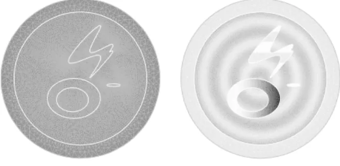
of choosing this pattern is to demonstrate that the reconstruction methods are very effective for a large variety of conductivities. The conductivity distribution is presented on the Figure 1. The simulations are done using the partial differential equation solver FreeFem++ [7].
Figure 1: Conductivity Distribution.
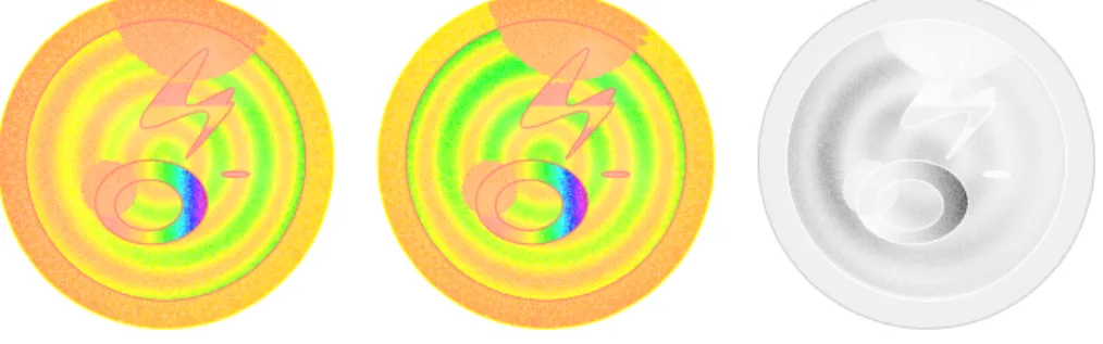
Figure 2 shows the result of the reconstruction when perfect measurements (with ’infinite’ precisions) are available. We use two different Dirichlet boundary data, gx = 2 + x/6 and
gy= 2+y/6. In the first approach proposed in Section 3.1, this is implemented by alternating
the procedures with gxand gy. In the optimal control approach, this corresponds to simply
adding the contribution of both correctors. In both cases, the boundary data are positive, which implies the positivity of u in the domain Ω. The initial guess is depicted on the left: it is equal to 1 everywhere. The right picture represents the reconstructed conductivity after three iterations. A 7 digit accuracy in L2
norm and in L∞ norm is reached after five
iterations.
Figure 2: Perfect reconstruction test. From left to right, the initial guess, the reconstructed conductivity after three iterations
To document the effectiveness of our approach in the case of partial data, we perturb the measure data. We add 5% noise to the measured data, and we destroy the data on two
elliptical subdomains, replacing it by 1. If we use solve iteratively, using alternatively the (perturbed) data corresponding to gxor gy, the algorithm cycles after fives iterations. This
is because we are trying to match mismatched data : the minimum corresponding to gxdata
is not the same as the one corresponding to gy, because of the perturbations we applied to
both data sets. The results are presented in Figure 3.
Figure 3: Perturbed reconstruction test. From left to right, the measured data for gxand gy, and
the reconstructed conductivity after five iterations
Note that the pattern is recognizable from the data E itself. This may be expected: thanks to De Giorgi-Nash estimates, the potential u is continuous, thus the data displays the discontinuities of γ. However, the value of γ cannot be read from the data. The local character of the minimization procedure is striking. The solution does not seem to be affected by a substantial loss of data. If we limit the minimization procedure to the area outside the elliptical subdomains instead of considering false data, the optimal control procedure converges to a non-zero minimum, which is due to the background noise. The reconstructed pattern is very similar to the one presented in Figure 3.
4.2
Magneto-Acoustic Tomographies with Incomplete Data
Suppose that the measurements of ∂pz/∂ν(x, t) are only done on a part Γ of the boundary
∂Ω. Suppose that T and Γ are such that they geometrically control Ω, which roughly means that every geometrical optic ray, starting at any point x ∈ Ω, at time t = 0, hits Γ before time T at a nondiffractive point; see [3]. Let β ∈ C∞
0 (Ω) be a cutoff function such that
β(x) ≡ 1 in a subdomain Ω′ of Ω. Following [1], we construct by the geometrical control
method a function ev(x, t) satisfying (3.13), the initial condition ev(x, 0) = β(x)vy(x, 0) (vy
given by (3.16)), the boundary condition ev = 0 on ∂Ω \ Γ, and the final conditions (3.14). The reconstruction formulae (3.26) and (3.27) should be replaced by
cγ(z) ≈ −2cs|z − y| 2 r2 Z T 0 Z Γ ∂pz ∂ν (x, t)(ev(x, t) + ev(x, −t)) dσ(x) dt, (4.1) and Z T 0 Z Γ ∂pz ∂ν (x, t)(ev(x, t) + ev(x, −t)) dσ(x) dt = c (y − z) · e 4π|z − y|3. (4.2)
5
Concluding Remarks
In this paper, we have proposed two algorithms for solving the inverse problem in vibration potential tomography. Both algorithms are based on transforming the conductivity equation into a nonlinear PDE. The first one follows from a perturbative approach while the second one follows an optimal control approach and can be applied to the case of incomplete data. It should be emphasized that from (2.4), an alternative way for solving the VPT problem is to first obtain j = γ|∇v| in each D and then to replace γ by j/|∇v| in the conductivity equation (2.1). This yields to exactly the same nonlinear problem as the one extensively investigated by Seo’s group for Magnetic Resonance Electrical Impedance Tomography (MREIT). An efficient algorithm for solving the inverse problem in MREIT is the so-called J−substitution algorithm. See for instance [9, 10]. We believe that if we restrict the resolution in the J−substitution algorithm to the size of D, it would lead to the same quality of conductivity images as the one provided in this paper. However, the algorithms developed here for VPT are simpler and use only one current.
For magneto-acoustic tomography with magnetic induction, we provided explicit inver-sion formulae. Magneto-acoustic tomography transforms the inverse conductivity problem into a much simpler inverse source problem. Because of the acoustic boundary conditions, the spherical Radon inverse transform can not be applied. Our approach is to make an ap-propriate averaging of the measurements by using particular solutions to the wave equation. Our approach extends easily to the case where only a part of the boundary is accessible.
It is worth noticing that our approach for the magneto-acoustic tomography can be used in acoustic imaging (see [19] for a review of the current state-of-the-art of photo-acoustic imaging). This will be discussed in a forthcoming paper. We also intend to gen-eralize our inversion formula to the case where the medium is acoustically inhomogeneous (contains small acoustical scatterers).
References
[1] H. Ammari, An inverse initial boundary value problem for the wave equation in the presence of imperfections of small volume, SIAM J. Control Optim., 41 (2002), 1194– 1211.
[2] H. Ammari, E. Bonnetier, Y. Capdeboscq, M. Tanter, and M. Fink, Electrical impedance tomography by elastic deformation, SIAM J. Appl. Math., to appear. [3] C. Bardos, G. Lebeau, and J. Rauch, Sharp sufficient conditions for the observation,
control, and stabilization of waves from the boundary, SIAM J. Control Optim., 30 (1992), 1024-1065.
[4] Y. Capdeboscq, J. Fehrenbach, F. de Gournay, and O. Kavian, An optimal control approach to imaging by modification, preprint.
[5] F.G. Friedlander, The Wave Equation on a Curved Space-Time, Cambridge University Press, Cambridge, 1975.
[7] F. Hetch, O. Pironneau, K. Ohtsuka and A. Le Hyaric, FreeFem++, http://www.freefem.org, 2007.
[8] M.R. Islam and B.C. Towe, Bioelectric current image reconstruction from magneto-acoustic measurements, IEEE Trans. Med. Img. 7 (1988), 386-391.
[9] S. Kim, O. Kwon, J.K. Seo, and J.R. Yoon, On a nonlinear partial differential equation arising in magnetic resonance electrical impedance imaging, SIAM J. Math. Anal., 34 (2002), 511–526.
[10] Y.J. Kim, O. Kwon, J.K. Seo, and E.J. Woo, Uniqueness and convergence of conduc-tivity image reconstruction in magnetic resonance electrical impedance tomography, Inverse Problems, 19 (2003), 1213–1225.
[11] O. Kwon, J.K. Seo, and J.R. Yoon, A real-time algorithm for the location search of discontinuous conductivities with one measurement, Comm. Pure Appl. Math., 55 (2002), 1–29.
[12] X. Li, Y. Xu, and B. He, Magnetoacoustic tomography with magnetic induction for imaging electrical impedance of biological tissue, J. Appl. Phys., 99 (2006), Art. No. 066112.
[13] X. Li, Y. Xu, and B. He, Imaging electrical impedance from acoustic measurements by means of magnetoacoustic tomography with magnetic induction (MAT-MI), IEEE Transactions on Biomed. Eng., 54 (2007), 323-330.
[14] A. Montalibet, J. Jossinet, A. Matias, and D. Cathignol, Electric current generated by ultrasonically induced Lorentz force in biological media, Medical Biol. Eng. Comput., 39 (2001), 15–20.
[15] B.J. Roth and P.J. Basser, A model of the stimulation of a nerve fiber by electromagnetic induction, IEEE Trans. Biomed. Eng., 37 (1990), 588-597.
[16] B.J. Roth, P.J. Basser, and J.P. Jr Wikswo, A theoretical model for magneto-acoustic imaging of bioelectric currents, IEEE Trans. Biomed. Eng., 41 (1994), 723-728. [17] H. Wen, J. Shah, and Balaban, An imaging method using the interaction between
ultrasound and magnetic field, Proc. IEEE Ultrasonics Symp. (1997), 1407–1410. [18] H. Wen, J. Shah, and Balaban, Hall effect imaging, IEEE Trans. Biomed. Eng., 45
(1998), 119–124.
[19] M. Xua and L.V. Wang, Photoacoustic imaging in biomedicine, Review of Scientific Instruments 77, 041101, 2006.