Communication in the presence of additive gaussian noise

DOCUMIT RlOOKl 6-41,_ o. ' 1,;, ro . lt t DOg} :N M-O-G

ab;

La-o0 be-Y45;$r O 'Aectronic8

~'~s~ac us I, 8titute of TechnolOgy

COMMUNICATION IN THE PRESENCE OF ADDITIVE

GAUSSIAN NOISE

F. A. MULLER

LOSK

a

9~~~~~~~~~~~~~~~~~~~~~_1

TECHNICAL REPORT NO. 244

MAY 27, 1953

RESEARCH LABORATORY OF ELECTRONICS

MASSACHUSETTS INSTITUTE OF TECHNOLOGY CAMBRIDGE, MASSACHUSETTS

I

The Research Laboratory of Electronics is an interdepart-mental laboratory of the Department of Electrical Engineering and the Department of Physics.

The research reported in this document was made possible in part by support extended the Massachusetts Institute of Tech-nology, Research Laboratory of Electronics, jointly by the Army Signal Corps, the Navy Department (Office of Naval Research), and the Air Force (Office of Scientific Research, Air Research and Development Command), under Signal Corps Contract DA36-039 sc-100, Project 8-102B-0; Department of the Army Project 3-99-10-022.

MASSACHUSETTS INSTITUTE OF TECHNOLOGY RESEARCH LABORATORY OF ELECTRONICS

Technical Report No. 244 May 27, 1953

COMMUNICATION IN THE PRESENCE OF ADDITIVE GAUSSIAN NOISE F. A. Muller

Abstract

This report presents an analysis of the properties of finite segments of noise taken from correlated gaussian noise. This analysis is applied to the problem of optimal detection of signals when a communication channel adds gaussian noise and introduces a linear distortion. Some specific examples are discussed briefly.

COMMUNICATION IN THE PRESENCE OF ADDITIVE GAUSSIAN NOISE

I. INTRODUCTION

This report will discuss systems of communication in which the symbols to be trans-mitted are represented by signal functions that are limited to consecutive intervals in time. These signals are disturbed by the addition of correlated gaussian noise. The problem is to compute a posteriori probabilities of transmitted symbols when the received signal and the a priori probabilities are known (1, 2). As correlated gaussian noise shows an autocorrelation over finite times, the a posteriori probabilities of dif-ferent symbols in a sequence will be statistically dependent when the a priori probabili-ties of these symbols are statistically independent. Although this dependence is a part

of the received information, it is difficult to make practical use of it. In this report, therefore, the condition will be imposed that the procedure of computing a posteriori probabilities for the symbol transmitted in a particular interval must be independent of the choice of all other symbols in a sequence. This condition may be further justified

by the fact that the use of the statistical dependence of subsequent symbols as part of the received information would mean the use of a larger alphabet than had been agreed upon. A still sharper restriction will be placed upon the procedure of the detection;

namely, that only the signal plus noise received in its own interval may be used, and that, therefore, no extrapolation of the noise from neighboring intervals is allowed.

This condition is indicated when nothing is known about the signal outside the interval (this situation is often encountered when physical measurements are performed); or when, at least, the possible signals in neighboring intervals show a great variety, as they will do in communication systems using a large alphabet.

II. DESCRIPTION OF A SEGMENT OF CORRELATED GAUSSIAN NOISE

The procedure for analysis will be given here only in a rough physical outline. A sharp analysis of the necessary mathematics may be found in von Neumann's work (3). An exhaustive treatment of the mathematical statistics of very similar problems is given by Grenander (4).

It will be necessary to have an appropriate description of the segment of noise that the channel adds to the signal. One possibility would be to give the statistical properties

of the coefficients n of the Fourier series analysis. These coefficients may be seen as coordinates in a space with an infinite number of dimensions. Each function is repre-sented by a point in this space. An ensemble of functions is reprerepre-sented by an ensemble of points. A gaussian ensemble is determined by a density function

P = exp

1

A n n) (1)

The coefficient A determines the variance of n ; the coefficient A, v determines

the correlation of n and nV. In general this correlation will not be zero. Hyperplanes of constant density are determined by

An

nn= C

(2) )I, V

This is the equation of a multidimensional ellipsoid. When the axes of this ellipsoid are used as a new system of coordinates, the mixed terms will disappear from the density function, leaving

1 m

P = exp nm(3) m

The use of a new coordinate system indicates that we are no longer analyzing the noise in sines and cosines, but in a different, complete set of orthogonal functions. By using this new set of functions, we simplify the problem greatly. We shall call these functions the eigenfunctions of the problem. They are determined by the statistical properties of the noise and the length of the time interval.

The first problem is to find these eigenfunctions. They are orthogonal and assumed to be normalized:

+1/ZT

j12

Pi ~ dt = 6ij (4)

-1/2T

The analysis of a function F(t) is given by

F(t) = E fj j(t) (5)

For clarification of this statement, consider, for example, a short segment of noise that contains only very low frequencies. The segment will consist of a nearly straight line. Fourier analysis of this segment gives sine terms, beside a constant term. Inso-far as the approximation as a straight line is correct, the coefficients of all of these sine terms are proportional to only one stochastic variable. Therefore, the sine terms in this case will show a strong correlation.

**Each orthogonal coordinate system corresponds to a complete set of orthogonal functions. One of these complete sets is the set of 6-functions at all times. The analy-sis in terms of these 6-functions is trivial, and equal to defining the noise function in the time domain. The coefficients AM correspond in this case to the autocorrelation function.

Therefore +T/2 4i(t) F(t) dt = f

+T/2

4i(t) E fj qj(t) dt = f

/z

+T/2

=

fj

6ij

=fi=

-T/2 and of course with Eq. 5

+T/Z

e/-T/2

ti(t) F(t) dt = F(8)

Let N(t) be a section of duration T from a noise function from an ensemble of gaussian noise, characterized by the autocorrelation function . The set 'i must be chosen so that all correlations n. n will be zero for i j. Calculation of n. and n. with

Eq. 6 gives Eq. 6 gives +T/2 ninj =I -T/2

+T/2

,Ji(t) N(t) dt +T J-T/2 (8) qj(T) N(Tr) dT

or, by interchanging integrations and averaging, +T/2

ni nj = N(t) N(T) i(t) jp(T) dt dT

-T/2 and with the definition of

+T/2 ni nj= JT/2 +T/2 pi(t) dt fT/Z -T/2 §(t-T) tpj(T) dT

with the condition ninj ₁ = ij (₃ r-i (the axis length of the ellipsoid)₁

+T/2 13 i _J-T/2TiT/ +T/2 ~i(t) dt J/-T/2 +T/2 i -/2 +T/2 i(t) dt / .- /2 (t-T) j T dT (t-T) j dT

and with Eq. 4

4 2T/2 ora. 3~~~/ +T/2 T / 2 i(t) pj(t) dt (6) (7) (9) (10) (11) (12) (e--T) j(T) dT (13) ii(t) F(t) dt

indicating that the set of functions qi is a set of eigenfunctions of the integral equation, 2

Eq. 10, and that the variances i are the corresponding eigenvalues.

When the operator {T is defined by +T/2

T f(t) = T/ Eq. 13 may be written

(15) showing that the set of functions Pi is a set of eigenfunctions of the operator 4T and that

2

the variances .ri are the corresponding eigenvalues.

So far, Iqi(t) has only been defined for -T/2 < t < +T/2. When we define qti(t) = 0 for t < -T/2 and +T/2 < t, Eq. 13 may be written

+00

r

j t) IT(t) (16) m(t-T) j(T) dT where (14) IT(t) = for -T/2< t< +T/2 IT(t) = 0 for t < -T/2 and +T/2 Z

3 p(t)= IT(t) w00 Uj(t)

With the operator }0o defined by

+oo i~, f(t) =

f

The operator {T works on functions inside the interval -T/2 < t < +T/2; the operator o00 on functions in the entire time domain. Since r(T) is an even function, both AT and §00 are hermitian and their eigenvalues are, therefore, real. A complete set of eigen-functions of §0o are the sines and cosines. The eigenvalue as a function of the frequency therefore characterizes 0o-. This eigenvalue equals the power density 2 N(o) of the noise spectrum.

o00 cos t = 1

+co

{(t-O) cos wO dO =

f

4 (T) cOS o(T-+t) dT

+oo00

~(T) (Cos XT cos ot - sin XT sin ot) dT = cos ot

f

4T COS XT dT

or

t}

(17) (18) (19) +oo

100

(t-T) f() dT 2

a-i i(t) = T 'i(t)

and

cos t = 2s N(w) cos wt (20)

(The Wiener-Khinchine relation, the symmetry of i((T), and the assumption that ((T) -for T -+ co are used. )

The Heaviside operator with transfer function 2 N(js), which is constructed by sub-stituting -s2 = -(d/dt)2 for in 2r N(w), has the same set of eigenfunctions and eigen-values as

Jo0

and may therefore be identified with it.

1c 2 N(js) (21)

If N(w) is (or may be sufficiently approximated by) a rational function of Z, the

eigenfunctions and eigenvalues can be found by a fairly simple process. Equation 18 may be written

IT(t) (o - ri q i(t) = (22)

or

-0 <i>+i(t) = ni(t)

with

li(t) = 0 for t < -T/2 and +T/2 < t (23) and

9i(t) = 0 for -T/2 < t < +T/2

The behavior at the points ±T/2 will be specified later. Suppose n 21

Z

Cs 2 - =2r N(js) = =C(s) (24) 1=0 C (s2 ) 2 1 D(s) 2 (25) D C(s2) D(s ) [C(s2) - cr2 D(s2)] i(t) = D(s2) ni( t) (26)

The operators working in Eq. 26 on i and i are pure differential operators. Therefore

ai

must fulfill the conditions for both i and i in Eq. 23

ii(t) = 0 for every t except for t = T/2

At the points T/2, 6-functions and derivatives may exist. It may be shown easily that there is always a complete set of eigenfunctions that are either even or odd. We must therefore be able to find a complete set by assuming

i(t) = Ai(s) 6(t + T/2) + Ai(-s) 6(t - T/2) (27) 2

Ai(s) = E Ail s (28)

1=0

The value of r must be chosen so that it will be consistent with Eq. 11 which may be written, for i = j,

+oo00 +00oo

X i(t) ni(t)dt= C-2 ( ~ i(t) *D i(t) dt (29)

Whenever r 2n, this integral will diverge at the points t = +T/2. Therefore

r = 2n - 1 (30)

We may now try to determine the coefficients At from the conditions of Eq. 23 for ,ii and 'pi

Ai(s) Ai(-s)

ni(t) (s2) 86(t + T/2) + 2 6(t - T/2) (31) D(s D(ss2)

The pulse response corresponding to the operator Ai(s)/D(s ) may be found with Heaviside's expansion theorem. This theorem must be used in a form that gives an even pulse response (for example +(t)) for a symmetrical operator (for instance oO), that is, in a form giving the pulse response that is valid in the strip of convergence con-taining s = 0. Denoting the roots of D(s2) = 0 by sh and assuming that there are no

double roots, Heaviside's theorem may be written

D(s) h exp(sht) (32)

S=Sh with

E(X) = 0, X< 0; (0) = 2; (x) = 1, x> 0 (33)

Equation 31 may be written in the interval -T/2 < t < +T/2

0 = - E(Re(s))] d [Ai(s ] exp s(t + T/2) T (Re(s)) exp s(t -I[' [D(5 ] · (Re~s)d ds [D(s2 )]

S=S_h

(34) This requires

Ai(sh) = 0 (Re(sh) < 0) (35) and the identical condition

Pure imaginary roots do not exist as N(o) is bounded. Double roots require that Ai(sh)= 01

ds A(s) O [iRe(sh) < O] (36)

d-s Ai(sh) = 0 In this way we obtain n conditions for the Ail

Aio +AilSh +Aih+ ... = 0 Re(sh) _] (37) and eventually derivatives for multiple roots.

The same procedure gives, when applied to i(t),

= T/-E(Re(s))] [(t-+ dC _j o. D(s 2)] exp s(t + T/2)

k ds i

+ [(t - T/2) -E(Re(s))

Cs

2 ( D(s) exp s(t - T/2) (38)

ds [(s2) _ a2 D(1Z)

SSk(i) with Sk(ai), the roots of C(s2 ) - i D(s2 ) = 0.

The condition that i(t) be zero for t < -T/2 and +T/2 < t requires

Ai(sk) exp(skT/2) Ai(-sk) exp(-skT/2) = 0 (39) or

Ao cosh(skT/2) + A1lk sinh(skT/2)

+ Ask cosh(skT/2) + ... = 0 (for even i) (40) and

Ao sinh(skT/2) + Alsk cosh(skT/2)

+A sk sinh(skT/2) + . 0 (for odd

Ji)

(41)

For a double root, one of these has to be replaced by its derivative as shown in Eq. 36. In the set of Eq. 38, each equation is double; therefore, Eq. 38 represents 2n conditions. In total we have just as many equations as coefficients Ail. However, as these equations are homogeneous, in order to have a solution ' 0, the determinant of

2

these equations must be zero. This determinant is a function of o. and determines the

~~~~~~~~2

i~~~1

eigenvalues ori. It may be written easily for each application.

Double roots will occur only at discrete values of (Tr.. The determinant, set up in

1

the assumption of exclusive single roots, will indicate these values erroneously as eigenvalues. It will not be difficult to sift them out afterwards.

Fig. 1

An estimation of the number of eigenfunctions, with eigenvalues smaller than o-2, for an arbitrary example of a noise spectrum.

of Ai Substitution in Eq. 38 then gives the corresponding eigenfunction which may be

~ilf,~~~

2

normalized afterwards. The eigenvalues o.i are the result of the pure imaginary roots Pk which make the hyperbolic functions periodic. These pure imaginary roots may be found by drawing a horizontal line at height o- in the noise power spectrum (Fig. 1). The intersection points of this line with the power spectrum give the values of W k = sk

When a-2 is increased by such an amount that all values k travel together, on the aver-age, a distance of 4rr/T, both the even and the odd determinant will pass through zero; therefore, there will be, on the average, two eigenvalues in this interval. Only real roots for wk have to be considered, since all other roots move in pairs so that their influence on the determinant is approximately cancelled. Consequently, an estimate of the number of eigenvalues smaller than ac may be found by multiplying the total length Aw where c-2 > 2TT N(w) with T/2r. The main frequencies occurring in an eigenfunction with an eigenvalue of approximately a- are given by a- = 2r N(c).

III. CALCULATION OF PROBABILITIES

--4~

Suppose a signal Xk with components xki has been transmitted. The probability density of receiving a signal with components yi will be

(Yi - xki) e 2 o

)

(42) or Yi exp 2 P(Xk)= ( 1 exp(-Vkk + 2k) (43) i (2 (Ti) /2 with 2 V 1 Xki kk =Z2 (44) i 1C

and

i = ' EI

' Xki (45)

%k YZ Yi Xki

i i

These expressions for Vkk and %k may be interpreted as the dot product of Xk and Y respectively, with a vector Zk having components ki = Xki/Oi.

The corresponding time function

Zk(t) = k i (t) (46)

1 1

is the solution of an integral equation (Eq. 19):

+ T/2 X(t) =

kti

f(t-T)

j (T) dT /i . i 2 +T/2 _{(t -T) ki} i(T dT +T/Z = (t-T) Zk(T) d = Xk(t) (47)

-T/2

When the solution of this integral equation (Eq. 47) is not unique, the difference of two solutions is an eigenfunction with the eigenvalue zero of Eq. 13. This case, where the definition, Eq. 46, obviously makes no sense, would indicate that there are signals that are not disturbed by noise, and has, therefore, no practical impor-tance.

The computation of Zk(t) for a given Xk(t) may be carried out in a simpler way than by determining the eigenfunctions and using Eqs. 6 and 46. The process, leading from Eq. 13 to Eq. 23, may be applied to Eq. 47. This leads to

U(t) = 0 Z(t) (48)

with

Z(t) = 0 for t < -T/2 and +T/2 < t (49) and

U(t) = X(t) for -T/2 < t < +T/2 (50) where, for simplicity, the subscript k has been dropped.

In order to solve Eq. 48 it is again necessary to assume that the power density of the noise is a rational function of the frequency; therefore

n 2J Z C1 s 2 = P= = C(s ) Cl0 n 21D(s D D(2 1=0 A function V(t) can be defined

V(t) = D(s 2 ) U(t) = C(s 2) Z(t) with conditions for V(t)

V(t) = C(s2) Z(t) = 0 for t < -T/2 and +T/2 < t V(t) = D(s2 ) U(t) = D(s 2 ) X(t) for -T/2 < t < +T/2

(24)

(51)

}

(52) Addition of 6-functions and derivatives at t = + T/2 gives

V(t) = D(s2) X(t) + A(s) 6(t + T/2) + B(s) 6(t - T/2) (53) where A(s) and B(s) must again be determined from the conditions of Eqs. 49 and 50. Calculation of Z(t) = 1/C(s2) V(t) and U(t) = /D(s

)

V(t) with Heaviside's expansion theorem gives, with the conditions of Eqs. 49 and 50,

+T/2

A(sk) exp(skT/2) + B(sk) exp(-skT/2) = D(s2) T X(T) exp(-skT) dT

A(sh) = 0 (Re(sh) < 0)

B(sh) = 0 (Re(sh) > 0)

where sk are the zeros and sh are the poles of the system function N(as). A and B are allowed to be of the grade (2n - 1). Equation 54 allows calculation of the coefficients of

2n-I 2m-1

A(s)= Z A's and B(s) B sI

1=0 1=0

When A(s) and B(s) are known, Heaviside's theorem gives

Z(t)

= (C( 2

)

D(s2)

1/2k 1fT/2

exp(s

I(t-

T)) X(T) dT

+ A(s) exp(s(t + T/2)) + B(-s) exp(-s(t - T/2))

s=sk; Re(sk)< D

+

n * X(t)

n

The computation of Z may be simplified by splitting X(t) into an even and an odd and treating these parts separately; setting Aeven(s) = Beven(-s) and Aodd(s) = -B

(55)

part, odd(-s)

The dot product of two vectors is invariant under coordinate transformations +T/2 Ek _{i i}

=

k

_i pi(t) L(t) d(t) ; +T/T +T/2 +T/2 = k. ki 4i(t) L(t) dt t = K(t) L(t) dt · -T/2 J/2 and therefore +T/2

Vkk

2

f

Xk(t) Zk(t) dt

(56)

/2 and +T/2 1k2 Of, Y(t) Zk(t) dt (57) k=T/2

From Eq. 43 it follows that the a posteriori probability P(Xk kY) of the signal Xk with an a priori probability P(k) is (2)

P(Xk) exp(-Vkk + 2dk) P(Xk ) P(Xk) exp(-Vkk + 2k)

k

As k is obtained by a linear process from Zk, and Zk by a linear process from Xk, Ok

is a linear function of Xk(t) (for a given Y(t)). Therefore, when there are linear rela-tionships between the Xk(t), linear relarela-tionships also exist between the k. It will not be necessary in such cases to compute more correlation integrals (Eq. 21) than there are independent Xk(t). The rest of the dk may be found as linear combinations. In practice, this crosscorrelation will always be carried out by constructing a filter (or other linear physical devices) with pulse response Zk(T/2 - t) and then feeding Y(t) to it and sampling the output at the time T/2.

In a special case, which is often encountered in performing physical measurements, the possible signals all possess the same shape but different amplitude.

Xk(t) = k . Xl(t₎ (59)

where k is the quantity to be measured and Xl(t) is a given function of time. Most often k is continuous. It may be assumed that the a priori probability distribution P(k) is given.

Obviously

and +T/2 V k 2k2 Xl(t) Zl(t) dt = k V1 (61) T/2 +T/2 k k 2it Y(t) Zl(t) dt = 2 k 1 (62)

/2

Therefore, the a posteriori probability distribution of k will be

P(k) exp (k

V-P(k+ Y) = 12 (63)

P(k) exp 2 1 dk

When the a priori distribution is flat, the a posteriori distribution is gaussian with center value 41 k V (64) and variance 2 =1 (65) 11

Therefore, V1 1 may be interpreted as the signal-to-noise ratio for the signal Xl(t) when

the optimum filter is used to detect it.

When the optimum procedure is, in advance, assumed to be linear, the special case, described by Eq. 59, reduces to an optimum filtering problem. These optimum filters have been extensively dealt with in the literature (5, 6, 7, 8, 9). The work of Zadeh and Ragazzini (8) on finite memory filters gives the same results for the optimum filter as derived here. The mathematical methods, however, are slightly different.

IV. CHANNELS INTRODUCING LINEAR DISTORTION

The theory described so far may be used in connection with the problem of commu-nication through a channel that introduces a linear distortion. The situation is shown

schematically in Fig. 2. It is assumed that a sufficient approximation of the transfer function of the channel and of the power density of the noise is given as a rational function. At first, an additional restriction will be placed upon the channel transfer function: It will be assumed that it has no zeros on the imaginary axis or in the right half-plane. Under these circumstances the inverse network exists and may be used as a first step to the unravelling of the signal. This inverse filter multiplies the power density of the noise by [F(j,)/E(jw)]2. The problem reduces therefore to the problem

NOISE

TRANSMITTER

CHANNEL

RECEIVER

Fig. 2

A communication system introducing linear distortion and gaussian noise.

discussed in section I, with a noise power density [F(jw)/E(j)] 2 C( )/D(3), the equivalent noise spectrum at the transmitter. The function Z(t), which must be cross-correlated with the output of the inverse filter, may therefore be found. As a last step, the necessary practical outfit may be simplified by combining the filter F(s)/E(s) with the filter which performs the crosscorrelation, and making a physical device that realizes this combination to a sufficient degree of approximation.

The restriction on the location of the zeros of E(s)/F(s) will not be met in practical cases. In all but trivial communication channels, there will be a zero at = o, and often there will be one at o = 0. Strictly speaking, it is then no longer possible to carry out the inverse operation F(s)/E(s). The penalty for attempting this operation is that the noise power density found afterwards is no longer bounded. Therefore, the

auto-correlation function (t) does not exist and the calculation loses its sense.

We may, however, try to find the solution as a limit by solving the problem for the transfer function E(s)/F(s) + a, where a is a small positive real number tending towards zero. Although the autocorrelation function does not converge to a limit, the eigen-values and eigenfunctions do, with the exception of the eigenfunctions built up with the "forbidden" frequencies. The eigenvalues of these eigenfunctions increase proportion-ally with /a. Consequently, although the convergence of the set of eigenfunctions and eigenvalues is not uniform, the function Zk derived from any bounded Xk converges to a limit. This limit, Zk, a=0' pays no attention to the forbidden frequencies Xk contains. This is, of course, a physically sound procedure. It may, therefore, be assumed that this limit is the correct answer to the problem.

With a few minor alterations, the given procedure of computing the set of eigen-functions or the function Zk may be made to yield directly the limiting values. A zero at infinity means that the degree n of DI E2 is smaller than the degree 2m of C IF 2. The number of constants A then becomes m + n. A finite zero requires that Eqs. 35 and 54 hold also for Re(sh) = 0. With these additions the correct number of equations is obtained under all circumstances. The set of eigenfunctions found with this procedure is complete only for the received signals, not for the transmitted signals. The forbidden frequencies are lacking. This is, of course, not of practical importance, as one would not be interested in transmitting signals that cannot be received.

Although F(s)/E(s) is not realizable when E has zeros on the imaginary axis (as it

-13-N

2 7rAY

Fig. 3

Equivalent input noise for a sharply limited bandpass com-munication channel disturbed by uncorrelated noise.

would require an infinite gain for the corresponding frequencies), the combination of F(s)/E(s) and Z(t) is realizable, as the filter with impulse response Z(-t) has zeros on the imaginary axis where E(s) has them.

The second restriction imposed on E/F, the absence of zeros in the right half-plane, is necessary to insure the physical realizability of a network with the transfer function F/E. In practical cases, sometimes there will be zeros in the right half-plane; then the filter F/E is not realizable, nor are the combination filter of F/E and the correlation filter. If one again interprets the function of this combination as a cross-correlation (or weighted averaging), the difficulty lies in the fact that, in this process, the whole future is involved. This future part of the weighting function is necessary in order to cancel the influence of transmitted signals outside the time interval. The weight attached to this future goes exponentially to zero with increasing time. For practical purposes a sufficient solution is found by introducing a reasonable time delay and cutting off the rest of the future. Of course this process does not give correct prob-abilities or statistically independent results, but the deviation may be made as small as required. In most practical cases there will be no objection to the delay, which is necessary to obtain a close approximation of the ideal situation. When, however, a shorter delay is required, it will be necessary to reconsider the problem in order to be able to prescribe the changes to be made in the past section of the weighting function as a result of the cutoff of the future. This problem, however, remains outside the scope of this report.

V. EXAMPLES 1. COMMUNICATION

As a first example, it may be shown that the approach of this report leads to the points of view of Shannon (10) and Rice (11) when applied to the problem of communica-tion in a limited band, disturbed by uncorrelated noise. The equivalent input noise shows the spectrum (given in Fig. 3). The rule about the number of eigenfunctions for

-14-i oI g I I I I I I 0 U) Cd Q t, od4 CR ) oU) 0 .: o 0)-I s1 0 0 _ w SE Cd C 0 U Cd11Cd '4

~

_{o t}Cd - ) Cd m a ba E = tX O

~4

u , C o ., la 0 Q ( w x _-E Qb-2 0 *u -4 _{m O~~u"} I-~~~~~I a 10~~0_av U) c O¢ 0 E4 a)l 4) -4 Cd. a) n d4 Cd0 to . (2) Cd U)C a) b.0 a) a2b

-15-)<(

- C z 0_o o '·-I~~~~~~~~~~~~~~~~~~~~~~~~~~~~~~~~~~~~~~~~~~~~~~~~~~~~~~~~~~~~~~~~~~~~~~~~~~~~~~~~~~~~~

:::;

* 9 -k w ._ a b~1 I

ii'

>\- I

>(-~~~~~~~~~~~~~~-la

7 O,

>I

this case states that there are about 2TAv eigenfunctions, all with the same eigenvalue. In such a degenerated case, all linear combinations of eigenfunctions are again eigen-functions, and therefore any orthogonal set of about 2TAv functions, substantially

limited to the frequency band and time interval, may be used to describe the problem. Figure 4 shows the simplest example of a low- and high-cutoff communication chan-nel, disturbed by uncorrelated noise. Figure 5 shows the eigenvalues as a function of the basic time T. Figure 6 shows a number of the lowest eigenfunctions for T = 10RC.

The lowest eigenfunction gives, for a fixed energy, the largest number of distinguish-able levels (with a certain probability of error). When the average energy is limited, it seems, therefore, advisable to choose the transmitted signals as combinations of a number of the lower eigenfunctions. When only a small alphabet is allowed, the number of possibilities is limited and the best may be selected. It seems probable that when a large alphabet is allowed, a random distribution of signal points in accordance with Shannon's law (10), requiring that signal energy plus noise energy be constant as far as possible, will approach asymptotically the theoretical limit of the rate of transmission. A proof similar to the one Rice gave for the case of noncorrelated noise (11) would be very difficult here, as there is no spherical symmetry in the signal space.

2. PHYSICAL MEASUREMENTS

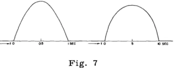
A typical example of the theory (12) is the point-by-point measurement of a quantity as a function of some parameter; for instance, the collector current in a mass spectrom-eter as a function of the magnet current. When a time T is available to dspectrom-etermine a point, the magnet current is kept constant during that time; therefore the signal, in this case the collector current, is constant during that interval. Nothing is known about the signal before and after the measuring time. The current measuring device usually is a voltage measuring instrument equipped with a current feedback. This feedback effects a transformation of the nearly uncorrelated noise of the voltage meter into a noise with a power density approximately proportional to 2 (at least for frequencies where the feedback is effective). The feedback resistor adds a constant power density. An addi-tional constant power density may serve as a first approximation for contact-potential

2 variations and flicker effect. The total noise spectrum becomes the form N = a2 + b. A typical example is a = 10 33 Asec 3; b = 10 33A sec. Optimal pulse responses for T = 1 sec and T = 10 sec are given in Fig. 7.

-t o 0.5 I SEC -- t o 5 10 SEC

Fig. 7

Two optimal pulse responses for a specific example of a current-measuring instrument.

Acknowledgment

The author is indebted to Professor R. M. Fano for many helpful discussions and constant encouragement of the research presented in this report.

References

1. P. M. Woodward, I. L. Davies: Phil. Mag. 41, 1001, 1950

2. R. M. Fano: Communication in the Presence of Additive Gaussian Noise, Sym-posium on Applications of Communication Theory, London, 1952

3. J. von Neumann: Die Mathematische Grundlagen der Quantenmechanik, Springer, Berlin, 1932

4. U. Grenander: Arkiv Mat. (Stockholm) 1, 195, 1950 5. D. O. North: Report PTR-6C, RCA Laboratories, 1943 6. H. den Hartog, F. A. Muller: Physica 13, 571, 1947 7. B. M. Dwork: Proc. I.R.E. 38, 771, 1950

8. L. A. Zadeh, J. R. Ragazzini: Proc. I.R.E. 40, 1223, 1952 9. K. Halbach: Helv. Phys. Acta 26, 65, 1953

10. C. E. Shannon: Proc. I.R.E. 37, 10, 1949 11. S. O. Rice: Bell System Tech. J. 29, 60, 1950

12. F. A. Muller: Measurement of Currents and Voltages with a Vibrating-plate Electrometer, Doctoral Thesis, University of Amsterdam, 1951

4