A Comparison of Plasma Ion Rotation and Magnetic Mode Rotation in Alcator C-Mod

DOE-ET-54512-342

A Comparison of Plasma Ion Rotation and Magnetic Mode Rotation in Alcator C-Mod

J.A. Sarlese

January 2002

Plasma Science and Fusion Center Massachusetts Institute of Technology

Cambridge, MA 02139 USA

This work was supported by the U.S. Department of Energy, Cooperative Grant No. DE-FC02-99ER54512. Reproduction, translation, publication, use and disposal, in whole or in part, by or for the United States government is permitted.

A Comparison of Plasma Ion Rotation and Magnetic Mode

Rotation in Alcator C-Mod

By

Justin A. Sarlese

B.S., Physics, U.S. Naval Academy (2000)

Submitted to the Department of Nuclear Engineering in partial fulfillment of the requirements for the degree of

Master of Science at the

MASSACHUSETTS INSTITUTE OF TECHNOLOGY

January 2002

Signature of Authoi

Certified by

Certified by

Accepted by

@ Massachusetts Institute of Technology

D menta Nuclear Engineering January 10, 2002

I

SV

Research Scientist, Plasma Science and Fusion Center

Thesis Supervisor

Ian Hutchinson Professor, Department of Nuclear Engineering Thesis Co-Supervisor

Jeffrey Coderre Associate Professor, Department of Nuclear Engineering Chairman, Departmental Graduate Committee

A Comparison of Plasma Ion Rotation and Magnetic Mode

Rotation in Alcator C-Mod

By

Justin A. Sarlese

Submitted to the Department of Nuclear Engineering on January 12, 2002, in partial fulfillment of the requirements for

the degree of Master of Science

ABSTRACT

There is still much to be learned about the ion toroidal rotation, the magnetic mode rotation, and the conditions under which they couple in a tokamak plasma. One way to better our understanding of these is through a comparison of the ion impurity rotation frequency and the sawtooth precursor frequency under various plasma conditions. In order to perform this analysis for a large number of experimental shots in Alcator C-Mod, an automated routine was written for determining the sawtooth precursor frequencies and loading these frequencies into a database, along with the ion impurity rotation frequencies and other plasma parameters taken at the times of the sawtooth precursors. It was determined that these frequencies agree most of the time, and their disagreement is in many cases the result of ion impurity rotation frequencies above 23kHz, sometimes the result of RF heating in excess of 4.2MW. According to the data in the database, there is a linear dependence between the two frequencies and WMHD/IP, as has been observed with previous research; however, comparable correlation exists between the frequencies and Op, ON, and WMHD/IP2. At the same time, there

appear to be candidate power laws for the two frequencies which include Op, ON, WMHD and IP, WMHD/IP, and WMHD/Ip2.

Thesis Supervisor: Joseph Snipes

Title: Research Scientist, Plasma Science and Fusion Center Thesis Co-Supervisor: Ian Hutchinson

Acknowledgments

Department of Nuclear Engineering Faculty: Prof. Ian Hutchinson, Prof. Ron Parker, Prof. Jeff Freidberg, Prof. Ambrosio Fasoli Alcator C-Mod Staff: Dr. Joseph Snipes, Dr. John Rice, Dr. Robert Granetz,

Dr. Earl Marmar, Dr. Rejean Boivin

Table of Contents

I.

Introduction

...

5

II.

Experimental Setup ...

12

III.

Computer Analysis ...

19

Purpose ...

19

General Overview...20

1. Primary Data Retrieval ...

21

2. Primary Data Display ...

23

3. Sawteeth Analysis ...

28

4. Secondary Data Retrieval & Display ... 31

5. Database Upload ...

31

6. Lessons Learned ...

34

IV.

Results of Data Analysis ...

37

Important Considerations ...

37

1. Comparison of Reliable Data with Previous

Experimental Results ...

38

2. Comparison of Sawtooth Precursor and Hirex

Frequencies ...

39

3. Plasma Confinement Mode and Rotation

Direction ...

41

4. Data Correlations ...

44

V.

Conclusions ...

54

Summary ...

54

Recommended Future Work ... 56

Appendix A: Flowcharts of IDL Routine and Tables of Variables ... .58

Appendix B: Fourier Analysis Techniques...

67

Appendix C: Frequency Agreement Plots...

70

Appendix D: Variable Correlation Analysis Techniques ... 77

Appendix E: Data Correlation Results ...

79

I.

Introduction

The amount of electricity used by the human race increases every year; however, the supply of fossil fuels, our main source of electricity, is expected to diminish within the next century [1]. This fact, as well as the amount of pollution produced by burning fossil fuels, demonstrates the eventual need to rely on an alternative primary source of electricity. The sun, the wind, and flowing water are all renewable, clean sources of electricity, but their production levels are limited by the climate. Nuclear fission, the splitting of Uranium and Plutonium isotopes, is yet another alternative source which has produced large amounts of electricity for many years, but unfortunately produces highly radioactive waste, and depends upon limited resources [2].

Nuclear fusion, however, another alternative source currently being researched, would produce large amounts of electricity with minimal damage to the environment and relies upon highly abundant resources. It involves the fusion of a deuterium nucleus and a tritium nucleus, a reaction which produces both a neutron and an alpha particle with 17.6 MeV (2.92 1012 _{J) of total kinetic energy. Based on some rough calculations, the world has}

been estimated to contain enough deuterium and lithium, a good source of tritium, to produce a total of -1019GJ of electricity [3], about 2.5- 107 times the world's annual energy

consumption in 1999 [4]. This makes nuclear fusion an attractive future alternative to fossil fuels as a primary source of electricity.

Unfortunately, in order to overcome the mutual repulsion between deuterium and tritium nuclei and fuse them, they must collide at very high relative velocities. This means they must be heated to very high temperatures (-1OKeV or -200,000,000*F) at which

gaseous deuterium and tritium will lose their electrons and form an ionized plasma. This adds many technological challenges because these fast moving particles, as well as their energy and momentum, must be confined for sufficient time without coming in contact with any physical material because they are so hot [5].

The magnetic confinement fusion community has been researching the use of magnetic fields to confine these particles, since ions and electrons are deterred from

commonly implemented in a tokamak', a device which uses helically shaped magnetic fields bent back onto themselves into the shape of a torus to confine a highly ionized plasma within a vacuum vessel. In order to create a nearly helical magnetic field, the tokamak utilizes large copper coils to externally apply a toroidal magnetic field and induces a toroidal current in the plasma to create a poloidal magnetic field. The toroidal current is induced with a transformer which ionizes the deuterium and/or tritium gasses in the vacuum vessel and can create currents in the resulting plasma on the order of mega amperes [7].

Unfortunately, the transformer is limited in its ability to keep the plasma hot. This is because transformers aren't steady state and because the plasma resistivity, il, is proportional to T , so at higher temperatures the transformer will provide less heating energy to the plasma [8]. Fortunately there are other ways of heating the plasma, including Neutral-Beam

Injection (NBI) and Radio Frequency (RF) heating. With NBI, high energy neutral particles are injected into the plasma where they collide with the ions and electrons, transferring their momentum to these particles. RF heating, on the other hand, uses intense radio waves, usually at the resonant frequency of hydrogen ions added to the plasma for this exact purpose. This is refered to as Ion Cyclotron Radio Frequency (ICRF) heating. These waves enter from the outer wall of the vessel, propagate inward, and are primarily absorbed by the plasma near the magnetic axis.

If the plasma in a tokamak behaved according to plan, the magnetic field lines would

remain fixed in helices and the particles, as well as their energy and momentum, would remain on or near the same constant flux surfaces long enough for the plasma to be self-sustaining. Unfortunately, the plasma in a tokamak is very chaotic, the magnetic field lines within the plasma rarely remain fixed, and the particles, their energy, and their momentum are lost from the plasma. In fact, the confinement times for these latter quantities are usually at least an order of magnitude less than they need to be for efficient energy production. This is partly the result of plasma instabilities on both the microscopic and macroscopic level.

The most troublesome instabilities in a tokamak plasma are those described by the magnetohydrodynamic (MHD) model of plasmas. These instabilities result from strong gradients in the current and pressure radial profiles or from abrupt changes in these gradients

Tokamak comes from the Russian acronym toroidalnaya kamera magnitnaya katushka which mean 'toroidal

induced by events in the vessel such as pellet injections, quick changes in the applied magnetic field, and foreign items falling into the plasma. MHD instabilities include ideal MHD modes, which will bend magnetic field lines and surfaces and even alter the shape of the plasma, and resistive modes, which may break the magnetic field lines and result in the formation of magnetic islands in the plasma [9]. Since these modes change the direction of magnetic field lines, they will usually increase particle, momentum, and energy transport toward the edge of the plasma.

For a circular, large aspect ratio tokamak, these modes take the form e inO+rnd where m and n are the poloidal and the toroidal mode numbers, respectively. One of the major

stabilizing effects which reduces these modes is the bending of magnetic field lines;

however, this effect is reduced on magnetic surfaces where the magnetic mode twists around the torus at the same rate as the magnetic field lines, especially for low-m modes. As a result, the strongest modes occur on surfaces where m/n = q and for n,n 3 [9]. Here 'q' is the

safety factor, defined as the number of toroidal turns per poloidal turn in the magnetic field lines on a constant flux surface.

One mode observed frequently in tokamak plasmas is the n=1,m=1 internal kink mode. It is responsible for the sawtooth behavior of the temperature time traces, seen in Figure 1.1. As the plasma core gets hotter, and the current density on the magnetic axis increases, the safety factor on the magnetic axis, qo, will drop. When qo falls below unity and a q=l surface arises within the plasma, an m=1, n=1 mode will grow within the q=1 surface. When the mode gets large enough, it will cause magnetic field lines to cross through the plasma core, resulting in a sudden increase in particle and energy transport away from the core. This will result in a sudden decrease or 'sawtooth crash' in the density and temperature of the plasma near the core and a sudden increase in the density and temperature of the plasma in the outer regions. It will also, according to the Kadomtsev model, reestablish a qo above unity and temporarily get rid of the m1 ,n= 1 internal kink mode [10]. Then the process will repeat itself. It should be noted, however, that plasma behavior which disagrees with the details of this model has been observed.

By constantly causing the tokamak plasma's core temperature and density to crash,

the n=1,m= 1 internal kink mode reduces the nuclear fusion reaction rate in the plasma core. The mode also results in a loss of energy from the plasma core. In many cases, the mode will

T. Time Trace from GPC at Plasma Core

0.92 0.94 0.96 0.98

time(s)

T. Time Trace from GPC away from Plasma Core

0.92 0.94 0.96 0,98

time(s)

Figure 1.1 - Timetraces of the electron temperature in Alcator C-Mod at the plasma core (top) and away from the plasma core (bottom) for shot 1010726022. This data comes from a grating polychromator (GPC) which diffracts the

electron cyclotron emission (ECE).

couple to other n=1,m>1 modes at other rational q-surfaces all the way out to the edge of the plasma, with the same rotation frequency [11]. Since particles within the magnetic islands usually travel at the same velocity as the island and energy transport is increased across the islands, this coupling can result in increased transport of plasma stored energy and

momentum [12]. Sometimes, this coupling will go all the way to the vessel wall, where the

3.5 3.0L-g 2.5 2.0 1.5 1.0 0.9 I I 2.0 1.00 1.B- I-1.6 1.4 1.21 0.90 I I 1.00 0

/I/,/

modes will couple to some stray magnetic field and induce eddy currents in the external structure. In some cases, as has been observed in other tokamaks and independently in Alcator C-Mod2_{, this will cause the modes to stop rotating or 'lock,' and lead to a disruption} shortly thereafter [13].

In many cases, the ions throughout the plasma will couple to these magnetic islands. Edery et al. has suggested this is the result of micro-tearing modes which surround the magnetic islands and stochastically transfer momentum across large regions of the plasma outside the islands. This theory does agree with many experimental observations, but it doesn't specify the plasma conditions under which this coupling occurs [14]. One of the goals of this project has been to determine those plasma conditions.

Often, an n=1,m=1 internal kink mode has a large amplitude for a millisecond or so before or after the sawtooth crash of the core density and temperature. If it is large enough to be observed at the edge of the plasma, its rotation frequency can be measured. The perturbed field at the edge will generally oscillate at the same frequency as the mode [15]. Frequencies observed immediately before and occasionally after sawtooth crashes are called the

'sawtooth precursor' and 'sawtooth postcursor' frequencies, respectively. From now on, any reference to sawtooth precursors in this paper will refer to both sawtooth precursor

frequencies and sawtooth postcursor frequencies, unless otherwise specified. Likewise, any reference to 'coupling' in this paper will refer to the coupling of the sawtooth precursor frequencies to the ion toroidal rotation frequencies.

Previous experiments at Alcator C-Mod have shown the impurity ion toroidal rotation frequency near the magnetic axis usually agrees with the sawtooth precursor frequency during purely Ohmic shots; however, during RF heating experiments, the former has been observed, on average, to be higher than the latter [16]. Previous studies and experiments have also found a strong correlation between large amplitude MHD modes and enhanced losses in plasma energy and ion toroidal momentum [12]. One goal of this project has been to check some of these correlations.

The sources, causes, and effects of the momentum responsible for the mode and ion rotation described above are still not totally understood. Many studies of plasma rotation

2 _{Alcator comes from the Italian acronym Alto Campo Torus which mean 'high field torus' because of its 12.0}

were done with experiments utilizing NBI heating, in which it was assumed the rotation was the result of momentum diffusion from the momentum input of the high energy neutrals. Studies with RF heating and no NBI, however, show rotation, leading some to believe there is an RF mechanism responsible for this rotation [17]. One theory is that ICRF heating shifts the resonant ion orbits radially inward which generates an Er that drives the toroidal rotation

[18]. However, additional experiments have shown considerable core rotation even without

any auxiliary heating and thus no obvious source of the momentum. These observations indicate that momentum transport isn't entirely diffusive [17].

Experiment has shown that rotation plays some role in the transition from low-to-high (L-to-H) confinement mode [19-22], is somehow associated with the formation of internal transport barriers (ITBs), and is correlated with energy confinement [23-26]. At the first L-to-H transition, the impurity ion toroidal rotation has been observed to switch from the counter-current to the co-current direction [23, 27-30]. Occasionally, the mode rotation appears to switch from the electron to the ion rotation direction just after the L-to-H

transition [31]. During some experiments, the shear in the flow velocity has been observed to affect the turbulence responsible for enhanced transport [32]. According to theory, when the velocity gradient, which is proportional to the ExB shearing rate, reaches a certain level, turbulence is stabilized and the ion thermal conductivity will fall to neoclassical levels, resulting in improved energy confinement [33-35]. Other experiments have shown that after the RF heating is turned off, the rotation will usually decay with a characteristic time comparable to the energy confinement time [36]. Previous studies have also shown the rotation to be proportional to the plasma stored energy and inversely proportional to the plasma current [37]. It has been an additional goal of this project to test some of these relationships.

The data for the analyses mentioned above came from a small number of

experimental shots and was handpicked from various databases. The goal of this project has been to perform a few of the same analyses, but to do this using an automated computer routine. The first stage of this project involved the development of a computer routine, described in detail in section 3, which finds sawtooth precursor frequencies and obtains data for various plasma parameters, including the ion toroidal rotation frequency, at the same time as each sawtooth precursor. Then the routine loads the data for each sawtooth precursor

timeslice into a database with thousands of timeslices. Even though this automation may result in a database with less accurate data, it makes it easier to analyze and check for relationships which may exist for a much wider range of shots.

The experimental setup for the Alcator C-Mod tokamak, the source of the

experimental data analyzed in this project, is explained in the next section. The third section includes a step-by-step description of the computer routine written for analyzing the raw data and loading it into the database. The fourth section describes the analysis of the database and the results of the analysis. The fifth section lists recommendation for future experiments and data analyses, followed by the conclusion in section six.

II. Experimental Setup

Alcator C-Mod is a high field (2.6T B-r 8T) compact (Ro ~ 0.67m, a - 0.22m, and

K 1.8) tokamak operating with plasma currents between 0.23 and 1.5MA and volume

averaged densities between approximately 0.2 and 6 - 10 20_m3_{. The plasma can be heated}

with up to three ICRF antennas (two 2-strap and one 4-strap) with a total source power of 8.0 MW using hydrogen minority heating [38-39]. Central ion and electron temperatures are typically between 2 and 5keV.

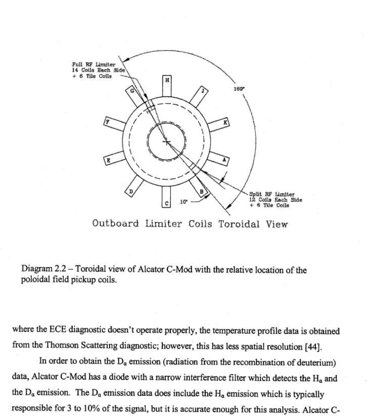
The magnetics data used to obtain the MHD mode frequency analysis come from a selection of five poloidal magnetic field pickup coils which measure dB,/dt. The coils are about 5cm from the outer separatrix, ranging from 4 to 11cm above the outer midplane, as shown in Diagram 2.1. Three sets of them are located on the sides of the outboard limiter between G- and H-ports while the other two are on the sides of the outboard limiter between

A- and B-ports of Alcator C-Mod. This is shown in Diagram 2.2. They are made up of a

kapton coated copper wire, wound around a ceramic spool. The coils are -12mm long and -8mm in diameter. Each coil has an effective area of -50cm2 and is covered by a stainless steel shield -. 4mm thick. The time resolution for these coils is about 1 gs and the dB,/dt resolution is -0.04T/s [31].

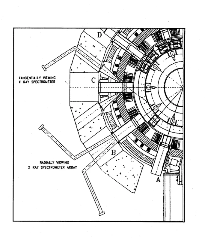
The data for the ion toroidal rotation frequency is taken from a von Hamos type crystal X ray spectrometer located between C and D ports with a line of sight along the magnetic axis, pointing in the counter-clockwise direction when looked upon from above

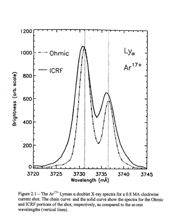
(see Diagram 2.3). This spectrometer measures the Doppler shifts of the Ar17+ La doublet lines (1s 1S1/2 --+ 2p

2_P

3/2 at 3.7311 A and 1S I S1 2 -+ 2p

2_{P12 at 3.73652A) from argon which} is routinely injected into the vessel through a piezoelectric valve, as shown in Figure 2.1. The time resolution for the data is 20ms and the frequency (toroidal velocity divided by toroidal circumference) resolution is -1.2kHz [40-42]. Sample timetraces for the data obtained from both this and the poloidal field pickup coils are shown in Figure 2.2.

Alcator C-Mod has two main diagnostics for obtaining temperature data. The temperature profile data is obtained from a grating polychromator (GPC) and a heterodyne radiometer which measure the X- and 0-mode electron cyclotron emission (ECE) [43]. The peak electron temperature data comes from another diagnostic which measures the

Magnetic Fluctuation Diagnostics

EF -4

EF-1 V

Poloidal Field

Pic -up coils

Diagram 2.1 - _{Poloidal cross-section of Alcator C-Mod, with poloidal field pickup coils in blue. The}

Full R iie 14 Calls"Eell ide

+ Tile Cails

Spit EFLKe

+ 6 Tile VbiUg Outboard Limiter Coils Toroidal View

Diagram 2.2 - Toroidal view of Alcator C-Mod with the relative location of the poloidal field pickup coils.

where the ECE diagnostic doesn't operate properly, the temperature profile data is obtained from the Thomson Scattering diagnostic; however, this has less spatial resolution [44].

In order to obtain the De emission (radiation from the recombination of deuterium) data, Alcator C-Mod has a diode with a narrow interference filter which detects the Ha and the De emission. The Da emission data does include the Ha emission which is typically responsible for 3 to 10% of the signal, but it is accurate enough for this analysis. Alcator

C-Mod also has other diodes used to obtain the visible Bremstrahlung emission for Zff [45] and the edge soft X-ray emission which is used to determine the plasma's confinement mode. The visible Bremstrahlung diode has a narrow interference filter as well while the edge soft x-ray diode uses a Beryllium window [44].

TANGENTIALLY VIEWING X RAY SPECTROMETER

RADIALLY VIEWING X RAY SPECTROMETER ARRAY

Diagram 2.3 - Toroidal view of Alcator C-Mod's X-ray spectrometers. Data from the upper, tangentially viewing, spectrometer was used in the analysis here.

The line averaged electron density data as well as the peak electron density data come from a two color interferometer (TCI) which is used to compare the phases of two CO2 laser beams, where one beam passes through the plasma and the other does not. These are used in

conjunction with a visible laser beam which is insensitive to the plasma yet sensitive to mirror vibrations and is used to subtract out the effect of such vibrations. The phase

1200

7

1000

-

Ohmic

_L

17+

ICRF

800

600

-200

1

20

3720

3725

3730

3735

3740

3745

Wavelength (mA)

Figure 2.1 - The Ar 17 _{Lyman a doublet X-ray spectra for a 0.8 MA clockwise}

current shot. The chain curve and the solid curve show the spectra for the Ohmic and ICRF portions of the shot, respectively, as compared to the at-rest

wavelengths (vertical lines).

difference between the two CO2 lasers is then used to determine the index of refraction of the

plasma from which the line averaged density can be obtained. This electron density data is also used in conjunction with the visible Bremstrahlung emission data and the electron temperature data, from either the ECE diagnostic or the Thomson scattering diagnostic, to obtain the plasma's effective charge [45].

Magnetics Data from coil BP05_GHK

I

-0.9 1.0 1.1

time(s)

Ion Toroidal Rotation Data from HIREX

0.9 1.0

time(s)

1.1

Figure 2.2 - Timetraces of the raw data from a poloidal magnetic field pickup coil (top) and the ion toroidal rotation frequency (bottom) in Alcator C-Mod for shot

1010726022.

The rest of the data used for this analysis is obtained from EFIT, a computer analysis code written by L.Lao at DIII-D and used at Alcator C-Mod for determining the MHD

80 60 U) 4., 40 20 0 -20 -40 -6D 0.8 1.2 20 15 10I N 5r 0 0.8 1.2

equilibrium of the plasma. This code takes data from poloidal field pickup coils, a Rogowski coil used to find Ip, and magnetic flux loops, and determines the shape of the constant flux surfaces in the vessel during each shot. From this routine, the plasma major radius, minor radius, and elongation can be obtained as well as the plasma stored energy, and the q-profile.

EFIT also computes the loop voltage and the upper and lower triangularities of the plasma

III. Computer Analysis

Purpose

The overall objective of this project is to sort through and use the raw data obtained from the detectors described in the previous section to efficiently and accurately perform some of the analyses described in the Introductory section. This requires an effective means of obtaining the sawtooth precursor frequencies for a large number of experimental shots. It also requires the ion toroidal rotation frequency, as well as a number of other plasma parameters at the same time as the precursors.

At the Joint European Torus (JET) and at Alcator C-Mod, some sawtooth precursor data has been obtained by hand; however, this process takes lots of time, and has only been done for a limited number of shots. In order improve upon this process, an automated IDL routine was developed for obtaining the sawtooth precursor frequencies. This routine is unable to determine the frequencies for all sawtooth precursors, but it is capable of distinguishing distinct sawtooth precursor oscillations of an n= 1 magnetic mode from oscillations coming from other modes or from noise. This is because the former will usually oscillate within a certain frequency range with an amplitude above a certain threshold. At the same time, the phase differences between these oscillations observed at different toroidal locations will be within a certain range.

In some circumstances, these frequencies can't be obtained and sometimes they are useless because certain raw data is unavailable; therefore, the routine distinguishes

experimental shots which have useful data from shots that don't have useful data.

The former will have hot plasmas which are stable for a certain amount of time, as well as strong magnetics and strong HIREX data during the same time period, while the latter don't. In other circumstances, the routine will obtain bad data. For this reason, the routine creates figures with the data it obtains so the user can determine the usefulness and validity of the data for each shot.

When the routine has finished these processes and has obtained sawtooth, hirex, and other plasma data for a certain shot, it goes on to load these data points into a database, where each set of data points is distinguished by the shot number and the time within the shot. This makes it easier to determine patterns and relationships in the data. The routine also saves the

figures it creates as 'gif files. These are useful for determining the validity of certain data points and for viewing any temporal behavior in the plasma.

General Overview of Routine

The experimental and analyzed data for the Alcator C-Mod experiment is maintained in a Model Data System Plus (MDSplus) data tree. The programming language used for analyzing the data in this tree is Interactive Data Language (IDL), version 5.4. The programs used for the analysis are written using Text Editor, part of the Common Desktop

Environment, version 1.0.

This routine uses one of three command files as well as nine main program files to extract and analyze data from the MDSplus data tree and then enter the results into an SQL database entitled 'sawtooth.' These files can be found in Alcator C-Mod's VMS cluster within the directory 'user 10: [jsarlese.automate].' The organization of the commands and procedures in this IDL automation routine is shown in chart A. 1 on page 59.

One of three command files can be used to start the automated routine. All three of these command files compile the nine program files used in the automated routine and then execute the procedure in EXECUTION.PRO; however, each one tells the succeeding procedures in the routine to treat the plotted data differently. PRINTFFTs.COM has the routine print out the plotted data, VIEWFFT.COM just has the routine plot the data on the computer screen, and LOAD_GIFS.COM has the routine load the plotted data into gif files. The gif files created are placed into the directory 'userl0:jsarlese.automate.giffiles],' and can be viewed using DISPLAY GIFs.COM which uses DISPLAYGIFs.PRO, both found in 'user10:[jsarlese.automate].'

Once in EXECUTION.PRO, the routine determines the shot or shots to analyze. It will ask the user to enter either a start date (a shot number minus the last three digits) or a

shot number. If the user enters a shot number, the routine will go on to perform the analysis for that particular shot only. If the user enters a start date, the routine will ask for an end date, create a shot list of experimental shots within the dates entered, and then begin the analysis of the first shot.

The analysis explained in detail in the next sections can be split into five segments. In the first part of the analysis, the routine will enter FFT4.PRO where it will retrieve data crucial to the analysis of the shot and determine whether or not the shot is worth analyzing.

The routine will then enter FFTTVPLOT4.PRO where it will analyze and plot some of the data retrieved in part one. After that, the routine will enter SAWTEETH4.PRO,

CROSSPOWER.PRO, and PLOTROTATION2.PRO where it will determine the sawtooth precursor and postcursor frequencies, and compare them to the HIREX rotation frequency. In the fifth part of the analysis, the routine will enter DATAPLOTS2.PRO where it will retrieve and plot various plasma parameters as a function of time. Following that, the routine will go into DATASETUP.PRO and WRITEDATA.PRO in which the routine will format the data for the database, then write it to the database.

3.1 - Primary Data Retrieval

Before the routine analyzes an experimental shot, it first checks to see whether the shot is worth analyzing and, if it is, the time window in which it is worth analyzing. A shot is only good for analysis when strong magnetics data, good HIREX rotation data, and a hot stable plasma exist at the same time. If any of these aren't present for a shot, the routine will skip to the next shot. This portion of the routine is found in the first half of FFT4.PRO which is outlined in Chart A.2.

The first data the routine retrieves is the magnetics data from the five poloidal field pickup coils. If data for any of the five coils is missing, the routine will skip to the next shot.

If less than 0.06% of the data points are above 20.OTesla/s, the data is too weak to have

distinct sawtooth precursors, so the routine will skip the shot. If more than 3.7% of the data points are above 20.OTesla/s, the magnetics data contains a large oscillating mode which

makes it too difficult to analyze; therefore, the routine will skip the shot.

The next piece of data the routine retrieves is the plasma current. If there is no current data, either the plasma never became stable or EFIT didn't work for the shot, so the shot will be skipped. If there is current data, the routine will determine the time window in which the current remains above 1OkA. If this time window is outside of the magnetics data time window or if the current never gets above 1 OkA, the routine will skip the shot.

Then the HIREX rotation data and the argon signal used to obtain the HIREX rotation data will be retrieved from the data tree. Once again, if any of this data isn't present the shot will be skipped. The routine will determine the time window within which the HIREX rotation data is present. After that it will come up with an argon signal data window which begins when the argon signal strength first gets above 80counts/s and ends when it finally

drops below 80counts/s for good. If either of these time windows are outside the magnetics time window, or outside the good plasma current window, the shot will be skipped. At the same time, if the argon signal strength doesn't get above 80counts/s for more than 50 points

(50ms) or the average argon signal strength is less than 80counts/s within the selected argon

signal data window, the routine will skip to the next shot. The routine also checks the average argon signal strength in a time window 20ms wide around each HIREX data point and throws out any points for which the average is below 80counts/s. If it ends up throwing out all the points, the shot will be skipped.

In some cases, the HIREX rotation data will show sharp and abrupt changes in the ion toroidal rotation frequency. Data points which exhibit such behavior are considered

unrealistic and are thrown out. The routine finds such sharp and abrupt changes by going through each HIREX data point and attempting to perform a fit on all the HIREX data points in a 90ms wide window around the selected data point. If the selected data point is at least 45ms from both edges of the HIREX data window, the fitting window will be set up so the selected data point is directly in the middle of the window; however, if the selected point is less than 45ms from either the beginning or the end of the HIREX data window, the fitting window will either start at the beginning or finish at the end of the HIREX data window, respectively. If the fitting window contains no points other than the selected point, no fit will be attempted and the point will be assigned a deviation of zero. If the fitting window contains

less than 5 points, the minimum number necessary for most IDL fitting functions, the routine will perform a linear fit on the points. Then it will record the point's deviation from the fit. If the fitting window contains five or more points, the routine will first attempt to perform a log

squares fit on the points. If this fails, it will then attempt a geometric fit, then attempt an exponential fit if the geometric fit fails. If both fail, it will attempt a gompertz fit and then a linear fit if the gompertz fitting routine doesn't work. Once the routine performs a successful fit, the selected point's deviation from the fit is recorded. HIREX points with a deviation greater than 10kHz are thrown out. If the points are scattered all over the place and are all thrown out, the shot will be skipped.

Next the routine will retrieve the disruption time, but if this data is missing the routine will not skip the shot. It will set the variable equal to -9.999e-09, commonly used in fusion databases to signify an unknown. However, if the disruption time is present and either less

than 0.3s, or comes before the start of the magnetics data, good current, or good HIREX rotation data windows, the shot will be skipped. If the shot passes this test, the shot routine will then use the 'good data' time windows described above, as well as the disruption time, if known, to determine the time window in which to analyze the shot.

Finally, the routine retrieves the ECE temperature data. Following this, the routine will enter FFTTVPLOT4.PRO where it will analyze and plot this magnetics data. Note that many of the thresholds required above work best for Alcator C-Mod data, but may need to be changed if this routine is to be used on data from a different tokamak.

3.2 - Primary Data Display

Since the automated routine doesn't work for every shot, once it has obtained the primary data it creates plots which display that data in a simple manner; therefore, an individual can judge the credibility of the analysis for each shot based on how the analysis done in the third section compares to the data in these plots. In FFTTVPLOT4.PRO, the routine performs a Fast-Fourier-Transform (FFT) analysis on the magnetics data and places the result into a 'tv' plot. The Fourier Transform is explained in Appendix B. Even though this FFT data isn't used in the sawtooth precursor analysis, the tv plot is useful for

determining whether the sawtooth precursor times and frequencies obtained in the next section are believable.

An outline of the program FFTTVPLOT4.PRO is shown in Chart A.3. When the routine enters this program, it first cuts down the magnetics data to the time window of interest, determined in the previous section, and then it begins the FFT analysis. The routine breaks each magnetics data array into mini-arrays of 512 points each, subtracts off the average of these mini-arrays, and then performs an FFT on each mini-array. After the FFT is taken, the routine determines the frequency components outside the frequency range of interest, which is currently set between 0 and 30kHz, and sets those components equal to zero. Then two things are done to the leftover FFT data.

A back FFT is performed on the data, and the results are plotted for all five coils. This

is useful to the user in determining the credibility of the shot analysis. If the plotted magnetics data for a shot has very small or no spikes, or shows a very large mode, for example, this will tell the user the data obtained for that shot is probably unreliable. On the other hand, if the plotted magnetics data has very sharp spikes, more than 3ms apart, with

distinct precursors in front of them and very little activity between them, this will tell the user the data for the shot may be reliable. An example of such magnetics data is shown in Figure

3.1. The routine also checks the maximum value for the backfiltered magnetics data on the

first coil. If the maximum value is less 20T/s, then the magnetics data associated with the frequencies of interest is too weak for a proper analysis and the shot is skipped.

The FFT data leftover after frequency filtering is also narrowed down to components corresponding to positive frequencies3 and undergoes n-mode filtering to eliminate frequency components not related to the n=1 modes. Two of the poloidal field pickup coils chosen are poloidally displaced, two are toroidally displaced over a small angle, and two are toroidally displaced over a large angle. The routine is only concerned with the cross-power of the two poloidally displaced coils, but uses the cross-phases of all three pairs of coils to determine what to do with the poloidal crosspowers. For this purpose, the routine takes the cross-powers and cross-phases of all three pairs of coils. The cross-power and cross-phase are both

explained in Appendix B.

Then the routine uses the cross-phases of the two coils which are displaced toroidally over a large angle to eliminate the frequency components, within each time window, which

are associated with even n-modes. Since these coils are on nearly opposite sides of the tokamak, any frequency components which have a cross-phase which is more than 40' different from the actual angle of displacement of the coils are assumed to be associated with even n-modes; consequently, the cross-powers of the poloidally displaced coils associated with those frequencies, within each time window, are set to zero.

Following that, the routine uses the cross-phases of the two coils which are displaced toroidally over a small angle to eliminate the frequency components not associated with the n=1 modes. The routine divides the cross-phases of the frequency components by the actual angle of displacement of the two coils to obtain n-mode numbers. Any frequency

components with an n-mode number greater than 2.0 are assumed to be associated with n*l modes; consequently, the cross-powers of the poloidally displaced coils associated with those frequencies, within each time window, are set to zero. This results in FFT data which only has nonzero values for positive frequencies associated with the n=1 modes.

3 IDL's FFT routine returns the data for both positive and negative frequencies. The automated routine here simply throws out the data for the negative frequencies.

T-C9 A E-2 N WI 1 , VO -i el q

A

It should be noted that the number of points in each time window, 512, the angle of deviation allowed for the cross-phase of the two distant coils, 40, and the mode deviation allowed for the mode of the two closer coils, 1.0, are all adjustable variables with names 'win,' 'dphi,' and 'dn,' respectively, in this routine. The values used here obtain the best results from Alcator C-Mod's magnetics data. When analyzing data from other magnetic confinement fusion devices, however these variables may need to be adjusted to obtain better results. A list of all the variables in the routine which might need to be changed for other experiments is shown in Table A. 1.

Next the routine loads this FFT data into a matrix, named 'out,' which has cross-powers as a function of both time and positive and negative frequencies. Those poloidal cross-powers associated with positive poloidal cross-phases, or rotation in the ion direction, are placed in the matrix with the positive frequencies. Those poloidal cross-powers

associated with negative poloidal cross-phases, or rotation in the electron direction, are placed in the matrix with the negative frequencies. The time associated with each column in the matrix is the time at the middle of the each FFT window.

After the matrix is constructed, the routine determines, within each FFT window, the root-mean-square of the magnetics signal from the first coil divided by the dominating frequency within that FFT window. This is a rough estimate of ABP and is used later in the routine.

The 'out' matrix is then reconfigured and plotted on a tv plot, shown in Figure 3.2, with time on the x-axis, frequency on the y-axis, and colors representing the intensity of the cross-powers. The temperature is also plotted below the tv plot with the same time scale. This plot is useful to the user in determining the reliability of the data analysis for each shot, partly because the sawtooth precursor times and frequencies obtained in the next section are plotted on top of the tv plot. If, for example, the tv plot is noisy with random colors all over the place and the sawtooth precursors are picked at times and frequencies with no distinctly intense cross-powers, this will tell the user the data obtained for that shot is probably unreliable. On the other hand, if the user sees a fairly blank tv plot, with the exception of spikes near the times of sawtooth crashes, and the sawtooth precursors are picked at times and frequencies near the edges of these spikes, this will tell the user the data obtained may be reliable.

5? R0 o>- N

liii I-IL' I U lii~ 144411 ILL1 111111111 H

1111111-~ a -4-4. - -~ N / N 0 111111111 U) AC C I I i VR m 0 C a 0 4 . 0 C> 1 - U 0 C to to -~C) OC) 'o 0 -- 0 o C)C)

After this is plotted, the routine enters SAWTEETH4.PRO (shown in Chart A.4) where it begins an analysis of the sawtooth precursor frequencies within the time window of interest.

3.3 - Sawtooth Analysis

In the effort to obtain the sawtooth precursor frequencies, the routine must first find the times of the sawtooth crashes. It does this by finding the magnetics spikes in the

unfiltered magnetics data from the first coil. First, it extracts all the magnetics data points for the coil where the signal goes above 15T/s. Then it goes through each point, checking 3ms in each direction to see if it's a local maximum, and throws it out if it isn't. The array of

sawtooth crash times that results is then taken into CROSSPOWER.PRO (shown in Chart

A.5) along with the unfiltered magnetics data.

Magnetics spikes which are too close to the edge of the analysis time window can't be properly analyzed; therefore, the routine throws these points out when it first enters CROSSPOWER.PRO. If it ends up throwing out all the points, then the shot is skipped.

When attempting to find the dominating sawtooth precursor frequencies, it is important that the routine not find the dominating frequency of the sawtooth spikes themselves. Therefore, the routine performs FFT analyses on six time windows, each 512 points wide, around each sawtooth spike, beginning 50 points (-50ps) away from the spike. Three of these time windows come before the spike, usually one after the other, and stop 50 points before it. The other three windows begin 50 points after the spike, usually one after the

other, and follow afterwards. In order to make this happen, the routine goes through each sawtooth crash time and finds the subscripts of the magnetics data for the starting times for the six FFT analysis windows that it will analyze around the crash. These subscripts are then loaded into a 1 -D array, six at a time. If the routine does not find enough points before the crash for three whole FFT analysis windows + 50 points, it will begin some of the windows

at the beginning of the magnetics window, resulting in repetitive and/or overlapping FFT analysis windows; however, all three windows will end at least 50points before the crash. Likewise, If the routine does not find enough points after the crash for three whole FFT analysis windows + 50 points, it will end some of the windows at the end of the magnetics

window, resulting in repetitive and/or overlapping FFT analysis windows; however, all three windows will begin at least 50 points after the crash.

Once these subscripts are obtained, the routine will perform an FFT analysis on each one of these windows, in a manner very similar to the FFT analysis in

FFTTVPLOT4.PRO. The frequency components corresponding to frequencies outside the frequency range of interest are set to zero, the negative frequency components are thrown out, and the frequency components corresponding to n;1 modes are also set to zero. Then, the poloidal powers are loaded into a matrix, this time named 'out4,' which has powers as a function of time and both positive and negative frequencies. Once again, cross-powers with cross-phases corresponding to rotation in the ion direction are placed into the matrix with the positive frequencies while cross-powers with cross-phases corresponding to rotation in the electron direction are placed into the matrix with the negative frequencies. Each set of six columns in this matrix corresponds to each set of six analysis windows around each sawtooth crash.

Then the routine returns to SAWTEETH4.PRO with the matrix and the updated array of sawtooth crash times. There the routine determines the time, frequency, and value of the maximum cross-power for each set of six cross-power spectra obtained around each sawtooth

crash. It also checks for selected points which are immediately succeeded ( 3ms) by another selected point with a greater cross-power. Such points are assumed to be the result of partial sawtooth crashes and are thrown out. The final result is a set of datapoints for each sawtooth precursor which includes the precursor time, frequency, and cross-power.

The routine then sends the leftover points through two filtering processes to eliminate points which may be the result of noise or other modes. After a careful analysis, it was determined that cross-powers from noise are usually much less than sawtooth precursor cross-powers and that the threshold for the latter is usually - 4.8T2/s2. Therefore, the routine

throws out selected points which have a cross-power below this threshold.

Since the rotation frequency of the n=1, m=1 kink mode isn't expected to change sharply and abruptly, any selected points which exhibit such behavior can't be reliable. In order to eliminate such points, the routine goes through each selected point and attempts to perform a fit on all of the points in a 90ms wide window around that point. If the point is at least 45ms from both edges of the magnetics time window, the fitting window will be set up with the selected point directly in the middle of the window; however, if the selected point is less than 45ms from either the beginning or the end of the magnetics time window, the fitting

window will either start at the beginning or finish at the end of the magnetics time window, respectively. If the fitting window contains no points other than the select point, no fit will be attempted and the point will be assigned an error equal to the frequency resolution of the FFT analysis which is -1.95kHz. If the fitting window contains less than 5 points, the minimum number necessary for most IDL fitting functions, the routine will perform a linear fit on the points. Then it will assign the selected point an error equal to either it's deviation from the fit, or the frequency resolution, whichever is greater. If the fitting window contains five or more points, the routine will attempt the same five fits, respectively, used to eliminate sharp and abrupt changes in the HIREX rotation data in the first section. Once the routine performs a successful fit, the selected point is assigned an error equal to either it's deviation from the fit or the frequency resolution, whichever is greater. Selected points assigned an error greater than three times the frequency resolution are then assumed to be unreliable and thrown out. If the points are scattered all over the place and are all thrown out, the shot will be skipped. The points which are retained are assumed to be the sawtooth precursors and are plotted on top of the tv plot, with error bars.

Then the routine goes into PLOTROTATION2.PRO, where it determines the maximum error in the HIREX rotation data. The maximum systematic error in the data is 10km/s and the maximum statistical error is 5km/s which correspond to -4.2kHz and

-2. 1kHz, respectively. The maximum percent error in the argon signal count rate is proportional to the reciprocal of the square root of the argon signal count rate, with a 10% error when the count rate is at 500 counts/s. The routine takes the maximum HIREX rotation frequency error resulting from these three sources of error to determine the maximum error for each HIREX data point.

Then the routine plots the HIREX rotation data with error bars over the tv plot with the sawtooth precursor data and opens a new graphics window where it plots the HIREX rotation frequency data points and the sawtooth precursor frequencies together on their own plot. In both cases, the routine uses different color triangles to distinguish the sawtooth postcursor frequencies, which are usually the minority, from sawtooth precursor frequencies.

3.4 - Secondary Data Retrieval & Display

In an effort to determine the plasma behavior associated with the coupling of the n=l ,m=1 kink mode to the plasma rotation, the routine also retrieves data for many plasma

characteristics within the magnetics analysis time window. Then the routine displays this data in a manner which makes it easy to compare the frequency coupling to the behavior of the plasma.

First, within FFT4.PRO, the routine uses the function 'efit rz2psi,' which relies upon FASTCOILSET2.PRO, to obtain the R and Z coordinates of the first poloidal field pickup coil. Then it uses the function 'coildata2' to find Bp at the first coil. This is then used with ABp, calculated in the second section, to obtain and plot AB/B, as a function of time.

Then the routine enters DATAPLOTS2.PRO which first obtains and plots BT,

pT,

and Ip, respectively. In order to obtain the plasma confinement mode, the routine uses L_ORH2.PRO which was created by Prof. Thomas Pedersen and uses edge soft X-ray emission to determine the confinement mode. The data from this is both plotted and used for finding the times of the L-to-H and H-to-L transitions. Then the routine continues to retrieve and plot the following: WMHD, dW/dt, POH, PRF, T

E, neo,<ne>, neo<ne>, _{Teo,<Te>, Teo/<Te>,}

dT,/dR @ q=l, D,, Zeff, and Voop,. Plots of these are shown in Figures 3.3 and 3.4. After that

the program returns to FFT4.PRO to reconfigure and load the data to the database. 3.5 - Database Upload

Before the data can be loaded into a database, it must first be arranged into timeslices, each of which is defined by a shot number and a precursor time, and has one value for each parameter. This is done in DATASETUP.PRO which converts all of the data to MKS units, except for the electron temperature which is in eV, and places it on the same timescale as the sawtooth precursors. It also obtains data for some additional plasma parameters including 'a' (minor radius), K, 8UPPER, 8LOWER, RMID, and q95.

For most of the plasma parameters, the routine simply uses linear interpolation to place them on the same timebase as the sawtooth precursors, but there are a few parameters for which this isn't the case. For each timeslice, for example, the routine finds the times of the L-to-H and H-to-L transitions closest to the precursor time. The routine also determines, for each coil, the root-mean-square of the backfiltered magnetics data within the FFT time window used to obtain the cross-power for the sawtooth precursor in each timeslice. It also

L m a .4-- 6 C q sq .9 9 9 ,, 1,, , , 1'., -C; C; c; C; ci - '- - 0 0D 0. 0 0**0 .in 64t U> ni d- *

I

E A C N -4- c -1 d R1

*A

Ig

a g

A

finds the confinement mode and the HIREX rotation error at a time closest to the precursor time for each timeslice. If the data for either of these variables ends before the precursor time, the routine will return a value of -9.999e-09 for the variable in that timeslice.

Next the routine enters WRITEDATA.PRO where it first multiplies the sawtooth precursor times by 1000000L to convert them to long integers, and subsequently checks the 'sawtooth' database to see if it contains any data for the shot being analyzed. If the database already contains data for that shot, it deletes that data. Then it will load the data it has into the database for that shot and those timeslices. A list of all the variables stored in the database is shown in Table A.2.

After that the routine will return to EXECUTION.PRO to obtain the number of the next shot to analyze and repeat the process. It should be noted that if at any time the routine decides to skip a shot because of bad data, no data, etc., FFT4.PRO has a section at the end which will tell it to look in the database for that shot and, if data exists for that shot, delete that shot from the database.

3.6 - Lessons Learned

When this routine was being created, there were a few analysis techniques which in theory seemed beneficial but in actuality proved to hinder the routine's ability to obtain good data at Alcator C-Mod. Some of these techniques may prove useful for those who use this routine at other magnetic confinement fusion labs. At the same time, it is important that other members of Alcator C-Mod who modify this routine don't make the same mistakes.

When SAWTEETH4.PRO was first created, it originally used the time derivative of the ECE electron temperature data to find the sawtooth crashes. There were three main problems with this. First, the temperature data had to be frequency filtered to eliminate the quick oscillations with large derivatives. This caused the routine to miss sawtooth crashes near the beginning and the end of the time window. Second, the derivative of the sawtooth crashes varied based upon the height and width of the sawteeth which can vary many times over the period of a single shot. Third, the ECE data was unreliable for many shots.

FFTTVPLOT4.PRO and CROSSPOWER.PRO originally added Hanning windows to the magnetics data. This added two problems to the data analysis. It would sometimes cause a frequency near the center of the Hanning window to become the dominant

frequency when the actual dominant frequency was closer to the edge of the window. It also added an envelope to the backfiltered magnetics data.

Since higher frequency components dominate the magnetics signal, at one time SAWTEETH4.PRO included a step which divided each frequency component of the 'out4' matrix by it's respective frequency, except for the zero frequency component. Unfortunately, this resulted in one serious problem. Since the routine determined the frequency of the maximum ABp component, there was no way to check the dB,/dt data to see if the results were correct; consequently, that step was eliminated. The program does still check for the maximum dBp/dt component, but it is possible to check the validity of the data obtained using the raw magnetics data. This means the analysis is more sensitive to higher frequencies, and tends to ignore lower frequency precursors.

When the routine was first being developed, it only used the cross-phases of two coils which were toroidally displaced by ~10* to eliminate the frequency components associated with the n*1 modes. Unfortunately, perturbations in the shape of the plasma and the

magnetic field lines can cause the phase difference seen by the two coils for many modes to vary by as much as 10*. As a result, if the mode deviation, 'dn,' allowed for a cross-power to be retained was small, it would throw out numerous n=1 components. On the other hand, if 'dn' was large enough to retain all the n=1 components, the routine would end up keeping n#l components as well, especially the n=0, n=2 components. This is why the program uses

the cross-phases of two coils nearly on opposite sides of the torus to eliminate the frequency components related to the n=even modes. This allows the use of a very high 'dn' when using the two closer coils to eliminate the ntl components.

During some experimental shots, high voltage trips have been known to occur in the von Hamos crystal X-ray spectrometer; consequently, any HIREX rotation data points obtained after one of these trips can't be trusted. When this occurs, the argon signal sharply drops; therefore, PLOTROTATION2.PRO originally included a section which took the time derivative of the argon signal and threw out any data points taken after the derivative went below a certain lower limit. Unfortunately, this doesn't work because the derivative of the argon signal during a voltage trip varies so much from shot to shot, in some cases even dropping below the derivative of the oscillations in a good argon signal. This makes it too difficult to establish an appropriate lower limit. However, since the argon signal strength

Mdb-after a voltage trip never rises above 80 counts/s, the first section of the routine does a good

IV. Results of Data Analysis

Important Considerations

Before the data in the 'Sawtooth' database can be analyzed, the bad data must first be filtered out. This is important because some experimental shots produce noisy data while others will produce unreliable data. At the same time, it is important that no unknowns, set to -9.999e-09, be used in analyses. Another concern is the fallibility of the automated routine. This is where the database variable 'reliable' and the gif files become important.

For every shot analyzed by the routine, 4 gif files are created with the plots produced in the analyses. Once the routine is done analyzing all the shots within the specified time interval, the user must then use the command file DISPLAYGIFs.COM to view these plots for the analyzed shots. Based on these plots the user must determine whether the data for a shot is reliable, marginal, or unreliable.

A shot with reliable data is one in which the routine has picked distinct sawtooth

precursors, the rotation data is realistic, and the magnetics data contains a small amount of noise. This means the 'tv' plot shows sawtooth precursors picked for frequencies and times where the cross-powers suddenly become intense immediately before or immediately after sawtooth crashes, as seen in the tv plot in Figure 3.2. This also means the time histories of both the sawtooth precursor and the Hirex frequencies don't exhibit any sharp or abrupt changes. At the same time, the magnetics data should contain very sharp spikes at the times of the sawtooth crashes, with growing oscillations either before or after them, and very little activity in between them, as seen in Figure 3.1.

A shot with unreliable data is one in which sawteeth crashes and precursors can't be

distinguished from noise, and/or the rotation data is unrealistic. This means that, through the entire shot, the magnetics signal is either very intense or never intense, so sawtooth spikes are either hidden beneath noise, or never present. A typical tv plot for a shot with unreliable data shows sawtooth precursors scattered in both time and frequency, nowhere near the time of sawtooth crashes, with a time history exhibiting large frequency changes in small amounts of time. If the Hirex data time trace also exhibits sharp and abrupt changes, then it is

unreliable.

A shot with marginal data has nearly reliable data, but may have a few sawtooth

Once the reliability of the data has been determined for each shot, the 'reliable' variable in the 'sawtooth' database must be set equal to 0, 1, or 2, for the timeslices within each shot if the data is considered unreliable, marginal, or reliable, respectively. This has been done for the analyzed shots for 1999, 2000, and 2001, using the program

RELIABLE.PRO. The 'sawtooth' database contains 1368 unreliable timeslices from 168 shots, 1904 marginal timeslices from 101 shots, and 5162 reliable timeslices from 208 shots.

When extracting the data from the database for analysis, the user can use a search string to limit the data to timeslices where reliable=2; however, other requirements should be added to this string to eliminate inaccurate and/or useless data. The user may need to limit the data to timeslices where certain variables remain within reasonable ranges. For example, if the user is performing an analysis with 'RMAJOR,' the major radius, the string must limit the data to timeslices with RMAJOR > 0.6, because EFIT occasionally produces unrealistic values for the major radius. At the same time, the user may need to eliminate timeslices where certain variables are unknown, and set equal to -9.999e-09. For example, if an analysis involves 'TEO,' the core electron temperature, the string needs to limit the data to timeslices with TEO > 0.

4.1 - Comparison of Reliable Data with Previous Experimental Results

Before the unique results obtained from any data analysis can be deemed credible, the user must first demonstrate that the reliable data obtained has patterns and relationships similar to those previously observed in data researched by respected scientists. According to studies by Dr. John Rice [37], Alcator C-Mod, the Hirex frequency increases linearly with

WMHD, the plasma stored energy, but with a steeper slope for smaller plasma currents. As shown in Figure 4.1, the reliable Hirex data in the sawtooth database shares the same relationship with WMHD. Based on this, Rice determined the Hirex Frequency scaled with

WMHD/IP. _{This was also mentioned in a paper by Prof. Ian Hutchinson [46], Alcator C-Mod,}

where he showed that the Hirex, as well as the sawtooth precursor frequency, scaled linearly

with WMHD/IP, with the exception of Hirex data for high power RF shots. This latter data had frequencies which were higher than the WMHD/IP scaling for the other frequencies. Figure 4.1 shows the Hirex and precursor frequencies from the sawtooth database for both Ohmic and RF shots, where an 'RF shot' is a shot with PRF/POHMIC greater than 10%. It demonstrates that

4x1 3x1 2x1 1x1

4

I

Figure 4.1 - The hirex frequency plotted against the plasma stored energy, for various levels of plasma current (upper), and both the hirex and sawtooth precursor frequencies plotted as a function of the stored energy over the plasma current (lower).

the frequency data in the database also scales with WMHD/IP, with the exception of some of the Hirex data for high power RF shots.

4.2 - Comparison of the Sawtooth Precursor and Hirex Frequencies

The sawtooth precursor frequencies and the hirex rotation frequencies are useful in determining the plasma conditions under which the ions couple to the magnetic modes in a

1.0x10 5 1.5x105 W.. (J) M 2.Ox 105 2.5x10r N I -V V 'I-, 0.25 0.20