HAL Id: hal-00295406
https://hal.archives-ouvertes.fr/hal-00295406
Submitted on 3 Mar 2004
HAL is a multi-disciplinary open access
archive for the deposit and dissemination of
sci-entific research documents, whether they are
pub-lished or not. The documents may come from
teaching and research institutions in France or
abroad, or from public or private research centers.
L’archive ouverte pluridisciplinaire HAL, est
destinée au dépôt et à la diffusion de documents
scientifiques de niveau recherche, publiés ou non,
émanant des établissements d’enseignement et de
recherche français ou étrangers, des laboratoires
publics ou privés.
Optimizing CO2 observing networks in the presence of
model error: results from TransCom 3
R. J. Rayner
To cite this version:
R. J. Rayner. Optimizing CO2 observing networks in the presence of model error: results from
TransCom 3. Atmospheric Chemistry and Physics, European Geosciences Union, 2004, 4 (2),
pp.413-421. �hal-00295406�
www.atmos-chem-phys.org/acp/4/413/
SRef-ID: 1680-7324/acp/2004-4-413
Chemistry
and Physics
Optimizing CO
2
observing networks in the presence of model error:
results from TransCom 3
P. J Rayner
CSIRO Atmospheric Research, Melbourne, Australia
Received: 29 July 2003 – Published in Atmos. Chem. Phys. Discuss.: 16 October 2003 Revised: 25 January 2004 – Accepted: 21 February 2004 – Published: 3 March 2004
Abstract. We use a genetic algorithm to construct optimal
observing networks of atmospheric CO2 concentration for
inverse determination of net sources. Optimal networks are those that produce a minimum in average posterior uncer-tainty plus a term representing the divergence among source estimates for different transport models. The addition of this last term modifies the choice of observing sites, leading to larger networks than would be chosen under the traditional estimated variance metric. Model-model differences behave like sub-grid heterogeneity and optimal networks try to av-erage over some of this. The optimization does not, how-ever, necessarily reject apparently difficult sites to model. Although the results are so conditioned on the experimen-tal set-up that the specific networks chosen are unlikely to be the best choices in the real world, the counter-intuitive behaviour of the optimization suggests the model error con-tribution should be taken into account when designing ob-serving networks. Finally we compare the flux and total un-certainty estimates from the optimal network with those from the TransCom 3 control case. The TransCom 3 control case performs well under the chosen uncertainty metric and the flux estimates are close to those from the optimal case. Thus the TransCom 3 findings would have been similar if mini-mizing the total uncertainty guided their network choice.
1 Introduction
Atmospheric tracer inversions, in which the atmospheric transport operator is inverted to deduce net sources from at-mospheric concentration observations, have been a widely-used tool in carbon cycle research in recent years, (e.g. Tans et al., 1990; Rayner et al., 1999; Bousquet et al., 2000; R¨odenbeck et al., 2003). Several previous studies (Rayner
Correspondence to: P. J. Rayner
(peter.rayner@csiro.au)
et al., 1996; Gloor et al., 2000; Patra and Maksyutov, 2002) have sought to suggest optimal extensions or reconfigura-tions of the atmospheric sampling network used in such stud-ies. The general method was to calculate some quantity rep-resenting the uncertainty in estimates of net source. This quantity is a function of the choice of observing network (among other things). The authors then used an optimization procedure to minimize their chosen quantity with respect to the network. The studies were generally interested in opti-mal extensions to the network and so were considering sta-tions where no data had yet been gathered. They relied on the general property of linear inverse problems that poste-rior uncertainties in unknowns do not rely on the values of data but only their error statistics. These error statistics are hard to infer even with data to analyze since the separation of signal and noise requires a statistical model of the obser-vations, often chosen ad hoc and a priori. Gloor et al. (2000) showed that this choice of error model had a great impact on the choice of desirable locations.
The network design studies have not yet been able to of-fer specific advice on observational sites although they have been instructive about the behaviour of the observing sys-tem. The reason is twofold. Firstly, the network returned by any optimization depends critically on the numerical quan-tity we optimize; the answer depends on the question. This was shown by Rayner et al. (1996) who performed optimiza-tions of two apparently similar quantities and suggested com-pletely different networks. Secondly, the results of the net-work optimization studies depend heavily on the prior knowl-edge input to the procedure. This was demonstrated by Gloor et al. (2000) through the importance of the error model for observations. It is clear, too, that regions with low prior un-certainty will not be improved as much by additional obser-vations as those with large uncertainties.
The network design studies have generally sought to min-imize some distillation of the posterior uncertainty in esti-mated fluxes but there is another source of uncertainty in
414 P. J. Rayner: Optimizing n etworks and model error atmospheric inversions. The atmospheric transport models
used both in the inversion and network optimization studies have different properties and produce different simulations of atmospheric transport. Throughout the history of their use, there has been a concern that these models may produce dif-ferent inverse flux estimates. In a series of studies to probe this, Law et al. (1996) and Denning et al. (1999) (studying the forward problem) and Gurney et al. (2002, 2003) (studying the inverse problem) have looked at the impact of differences in modelled atmospheric transport. Gurney et al. (2002) compared two measures of uncertainty of estimated fluxes. The first was the conventional posterior uncertainty estimate produced by error propagation from the prior flux uncertainty and data uncertainty via the inverse transport operator. The second was the variance of estimated fluxes across the en-semble of transport models. Following their nomenclature we refer to these as the “within model” and “between model” uncertainties respectively. These are formally defined in Sec-tion 2. A reasonable measure of the total uncertainty of es-timated fluxes is the quadratic sum of these two error terms. We use this sum throughout this paper and refer to it hence-forth as the “total uncertainty”.
Some interesting assumptions underlie the choice of un-certainty metric. First, what quantity does it represent? The “within uncertainty” describes the variance of an ensemble of flux estimates if we choose an ensemble of realizations of the data governed by the data uncertainty. The “between uncertainty“ describes the variance of an ensemble of flux es-timates drawn from the population of which our set of trans-port models generates a sample distribution. Note this is not the same distribution of fluxes we would generate from the ensemble of models of which we have a sample. So the distri-bution described by the “total uncertainty” describes the vari-ance of an ensemble of flux estimates generated by choosing a single model and data realization at random. This is differ-ent from, for example, the ensemble of flux estimates repre-senting the mean across models. For that case the “between uncertainty” contribution would be smaller as expected from the formula for the standard error of the mean. The next assumption is that the “total uncertainty” can be generated by the quadratic sum of its two components. This assumes the statistical independence of the two ensembles. This is a reasonable assumption but one that cannot be explicitly ver-ified. Finally there are the assumptions about the probability distributions for the chosen quantities. For the “within un-certainty” this is the assumption of the normal distribution for data almost universal in tracer inversions. For the “be-tween uncertainty” the assumption is surprisingly weak. The calculation of the sample variance does not assume a normal distribution. The real assumption is that the sample variance equals the population variance. Again this cannot be verified but no other assumption seems reasonable. Finally there is almost certainly correlation among flux estimates for differ-ent regions but we consider only the pointwise estimates (see Eq. 1 and Eq. 2) so these do not affect the formulation.
Gurney et al. (2002) found that, for most regions, within-model uncertainty dominated between-within-model uncertainty. They drew the reasonable inference from this, that additional data would aid the constraint of estimated fluxes by reducing total uncertainty. It was not, however, the role of those stud-ies to address this question directly. Any additional stations may have been so difficult to model that the between model uncertainty would increase more than the within model un-certainty was decreased. Investigating these possibilities is the role of the present paper.
The outline of the paper is as follows. In Sect. 2 we de-scribe the combination of the genetic algorithm (GA) and synthesis inversion. Section 3 describes a series of networks optimized under different conditions, comparing them with the TransCom 3 network of Gurney et al. (2002). Section 4 compares the fluxes computed from the optimized network with those from Gurney et al. (2002).
2 Methodology
The network optimization procedure requires two compo-nents, an inversion algorithm to calculate the score for a given network under our chosen metric and an optimiza-tion procedure to minimize this quantity with respect to the choice of network. The inversion algorithm is exactly that of Gurney et al. (2003) and the same as for Gurney et al. (2002) with the addition of one extra transport model, mak-ing a total of 17. See those papers for details of participatmak-ing models. The inversion is simple and computationally inex-pensive since it estimates term mean sources from long-term mean data. This makes the set-up a good candidate for the genetic algorithm where many repeats of the scoring cal-culation must be performed.
We are interested in two quantities calculated by the inver-sion procedure,
within uncertainty = trace(CS) (1)
where CS is the posterior covariance matrix of source
esti-mates for the 22 regions in the inversion and the overbar is the average across the ensemble of models,
between uncertainty =
22
X
i=1
Var(Si) (2)
where Siis the posterior source estimate for region i and V ar
represents the variance over the ensemble of models. Finally we define
total uncertainty = between uncertainty + within uncertainty (3) Genetic algorithms are one of the classes of stochastic op-timization procedures used for nonlinear models. The term “model” here refers to any numerical algorithm which calcu-lates an output as a function of inputs. In our case, the model
calculates measures of uncertainty as a function of a set of station locations.
Genetic algorithms seek to optimize their objective func-tion not by improving a single solufunc-tion but rather by improv-ing an overall population. Improvements are made by seek-ing optimal combinations of members of this population and by adding random changes to this population. In this sense they duplicate the pairwise reproduction and mutation seen in many biological systems. For a short on-line introduction see http://csep1.phy.ornl.gov/CSEP/MO/MO.html and refer-ences contained therein. Genetic algorithms exist in many forms but have a few general features
– the algorithm maintains a population of potential
solu-tions
– a given member of the population is described by a list
of parameter values. In our case these are integers refer-ring to an indexed list of possible observing sites. There are 110 possible observing sites in this study so each member consists of a list of integers in the range 1–110. The length of the list is the size of the network we seek to optimize.
– The population is initialized with a set of random lists. – members of the population will
1. Exchange parameter values pairwise (termed crossing-over).
2. Have their parameter values randomly changed (mutate).
3. Be culled or compete according to some fitness cri-terion based on the cost function we are optimizing. 4. Be cloned or otherwise reproduce to rebuild the
population after culling,
– The above four processes constitute one step of the
ge-netic algorithm.
– the algorithm iterates allowing evolution of the
popula-tion towards an optimum value of the fitness criterion.
– Convergence is achieved when the best value of the cost
function available from the population has not improved for a number of iterations greater than the population size. We choose as the optimum solution the list that produces the optimum (in this case lowest) value of the cost function throughout the entire run.
Each of the four parts of the algorithm can be implemented in various ways. We detail the particular implementation of each step here. The probability of two members crossing over (analogous to breeding), mutation rates and the mech-anism by which members of the population compete are all chosen by the implementer of the algorithm and choices de-pend on the properties of the cost function. In the sim-ple imsim-plementation used here cross-over is imsim-plemented by
first randomly pairing all members of the population then deciding whether to interchange information according to a random decision x∈U (0, 1)<pxwhere pxis the cross-over
probability and U (0, 1) is the uniform probability distribu-tion on [0, 1]. Once cross-over is chosen, the two original members are replaced with offspring that have pairwise ran-dom combinations of their parameters. For each parameter offspring 1 has the value from parent 1 or 2 with 50% prob-ability and offspring 2 has the value from the other parent.
For the mutation step we examine each parameter in each member of the population. Again we choose a uniformly dis-tributed pseudorandom number and, if less than the specified mutation rate, we replace the parameter value with a value chosen at random from the set of possible values.
In the culling step we first sort the population according to their generated values of the cost function. We then assign a fitness F to each according to
F =1 − r −0.5
N (4)
where r is the ordinal ranking of the member and N is the population size. We then delete the member according to the rule
x ∈ U (0, 1) > F (5)
Thus lower ranked members (with respect to the cost func-tion) are more likely to be culled. It is noteworthy that no member is completely safe from culling since F 6=1.
On average, each cull step will remove half the population and this must be replaced. For this we choose, at random, one of the remaining members of the population. If a ran-dom number from U (0, 1) is less than the fitness calculated from Eq. (4) we copy this member to replace one of the culled members. This process continues until the population is re-filled. Sampling is with replacement so that a member with high fitness may be copied several times.
In general the method requires a trade-off between strong enough selection to allow convergence to an optimal solu-tion and maintaining enough diversity to avoid getting stuck in a local extremum. In our case this trade-off is performed by tuning the mutation rate. The other trade-offs are com-putational, the population size and the number of iterations. A larger population is always safer since it means higher di-versity is maintained while still giving very fit members a chance to propagate (since for large N , F →1 for the fittest member). For our case we choose a population of 200 using 500 iterations. By this time the population consists mostly of clones of the fittest member. In all the experiments we carried out the final cost function was the lowest throughout the run, that is the optimization did not visit then discard a superior solution. One optimization takes about six hours on a single Linux PC.
416 P. J. Rayner: Optimizing n etworks and model error
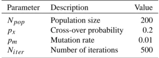
Table 1. Optimization parameters for genetic algorithm.
Parameter Description Value
Npop Population size 200 px Cross-over probability 0.2 pm Mutation rate 0.01 Nit er Number of iterations 500
2.1 Specific set-up
We assign each potential observing site an integer value. Sites considered are the 110 potentially used by Gurney et al. (2002). They chose 76 of these which met various crite-ria. The sites and data are taken from GLOBALVIEW-CO2
(2001). Each population member therefore consists of a list of these integer values. Data values and uncertainties are constructed by the same algorithm as in Gurney et al. (2002). Importantly, one station can occur many times in an optimal list but we do not include the correction to data uncertainty to account for this as used by Gurney et al. (2002). Therefore the second station at a location contributes as much informa-tion as the first. We also wish to test the possibility that the current network is too large to optimize total uncertainty. We therefore add 20 “null” stations which have zero responses to sources from all regions.
Values for the tunable parameters in the GA are shown in Table 1.
pm is of particular interest. Recall that it represents the
probability of a given value being altered. A simple binomial probability calculation demonstrates that, for our control 76 station case, this value of pmyields a probability of 54% that
a given member will be altered in the mutation step and a 19% probability that a given member will have more than one value altered. This is much higher than usual implemen-tations of a GA but our tests below found it to be an optimal value.
2.2 Testing the algorithm
Usually it is hard to design a test for a GA since we rarely know the optimal value. We could, however, construct a test here. The between-model case is uninteresting on its own but does provide a useful test. In a Bayesian inversion this metric will be minimized if the responses approach zero. The inclu-sion of the null stations in our potential network allowed us to test this. After 500 iterations the 76 station case produced a between-model variance of 0.01 (GtCy−1)2. There were still three real stations left, in the optimal lists, the rest all being null stations. We regarded this as acceptable and used this configuration throughout the real experiments.
Table 2. Uncertainty metrics in (GtCy−1)2for various optimized networks. The number at the end of the name is the possible number of sites in each network, the second column is the number of distinct sites chosen. In each case the bold-face number indicates the metric for which the network was optimized. The TransCom 3 control is also included for comparison.
Name Ndistinct Within Between Total
Total-76 40 6.26 1.96 8.22 Within-76 35 5.33 6.11 11.44 Total-110 46 5.77 2.10 7.87 Within-110 38 4.66 7.20 11.86 TransCom 3 62 7.05 3.27 10.32 3 Experiments
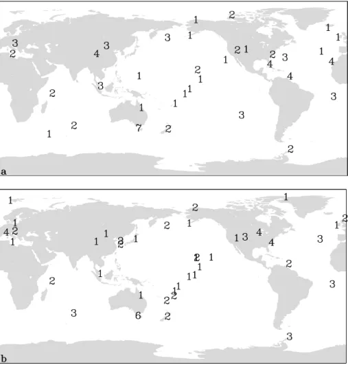
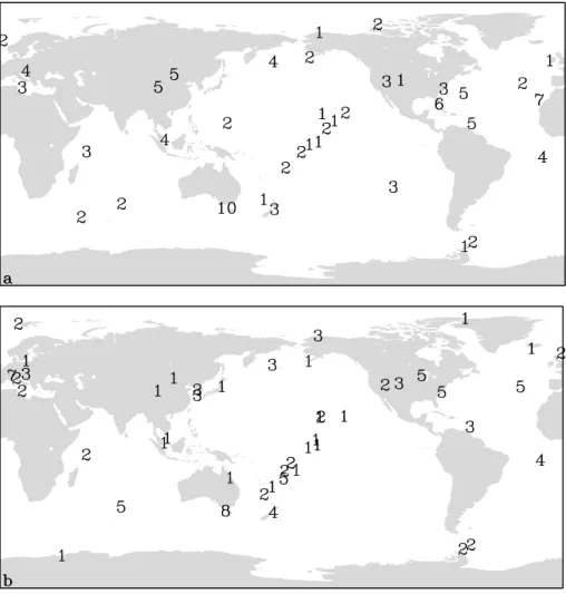
We performed experiments with two different sized works, the 76-station network as a comparison with the net-work of Gurney et al. (2002) and a 110-station netnet-work which is capable of covering the full list of available stations. In each case we performed optimizations with two metrics, either the “within uncertainty” (Eq. 1) or the “total uncer-tainty” (Eq. 3). The results are summarized in Table 2 and the four optimized networks are shown in Fig. 1 and Fig. 2.
The first thing to note about the various optimal networks is their relatively small size, especially for the “within” cases. This is largely a function of the resolution of the sources. To constrain 22 regions it is required to have at least 22 inde-pendent measurements. There is a tendency therefore for the “within” optimizations to gravitate to a selection of 22 sites that best constrain the 22 regions. In tests with a single model this was almost achieved, with networks of 26 sites being a common outcome. The complication of multiple models is that optimal choices for one model may not hold for oth-ers so that the optimization will choose more sites to give the strongest average constraint across all models. This was noted by Patra et al. (2003) who also showed an increase in chosen sites when several models were considered. That study could not duplicate our result since the optimization technique was not allowed to choose sites multiple times and the study was of additions to the current network rather than construction of networks from scratch. That study did demonstrate the dependence of the size of the network on the resolution of the source description. They noted a spreading of stations as they moved from the 22 regions used in this study to a higher resolution description with 42 land regions rather than the 11 land regions used here.
It is, a priori, unclear what to expect when moving from optimizing within to total uncertainty. If there is strong dis-agreement among model transport fields then we may expect a further shrinking of the network as some sites, although offering strong constraint on the fluxes, give highly diver-gent results from one model to another. In fact we observe
Fig. 1. Optimized networks for within-model (a) and total (b) uncertainty for a 76-site network. Numbers indicate the number of times the
site is included.
the opposite, with a growth in the size of the network for both the 76 and 110 station cases. It seems, in fact, that the optimization must counteract the model-model divergence caused by particular stations by averaging across a broader dataset. In that sense we may regard the model-model dif-ferences as some kind of heterogeneity. This is most clearly seen in Fig. 1 for Western Europe. Here the “within” opti-mization chose two sites while the “total” chose six. There is also some dispersal of sites around East Asia and the Pa-cific. From Table 2 it is clear that this dispersal produces a substantial reduction in “total” uncertainty without a large increase in “within” uncertainty. It would appear, therefore, that aggressive optimization of “within” uncertainty may ex-pose one to substantial model-model variability. This is ac-ceptable if one has a series of models with which to per-form inversions but this will not, generally, be the case. The case holds, even more dramatically, for the 110-site network. Here the lowest “within” uncertainty in Table 2 corresponds to the largest “total” uncertainty. Although the specifics of
these results will not, as discussed earlier, hold for a differ-ent set-up, we expect that this behaviour, with network di-versity acting to reduce large model-model variations in flux estimates, is a general result.
It is important to note that optimal networks do not include any of the “null” stations. This demonstrates that, even for the larger network size, the available information content is not saturated. This is the direct test of the inference drawn by Gurney et al. (2002) that extra measurements would reduce uncertainty, even when that uncertainty included a compo-nent caused by model-model variations. This result would stand even more strongly if we tried to solve for sources at greater spatial resolution.
In general, the “within” optimizations choose sites within or near each region to minimize atmospheric diffusion and hence maximize signals. Where there are no nearby stations well-connected by atmospheric flow to a source region this can produce some surprising choices. For example, both the within-76 and within-110 optimizations heavily weight the
418 P. J. Rayner: Optimizing n etworks and model error
Fig. 2. Optimized networks for within-model (a) and total (b) uncertainty for a 110-site network. Numbers indicate the number of times the
site is included.
upper levels of the Cape Grim aircraft profile. This site has the largest response to the South American source region of the available sites. The weakness of the constraint requires the optimization to invest many measurements at the site to simulate a high precision measurement, capable of seeing the small signals from such a distant source region. Rather than a comment on the utility of this site, such a choice points out the deficiencies in the rest of the network, with no other mea-surement site providing a good constraint on South America. The method we have used for the optimization of total un-certainty relies on the existence of real data at all potential observing sites. This is not particularly useful for planning a network. It is more useful if we can predict some of the impact of model-model variations using the properties of the response functions themselves. As an example, we consider three sites which are strongly favoured in the “within” opti-mization but do not appear in the “total” case. These are the Easter Island (EIC, 27◦S, 109◦W) (3 times), Izana, Canary Islands (IZO, 28◦ N, 16◦ W) (4 times) and Key Biscayne,
Florida (KEY, 26◦ N, 80◦ W) (4 times) sites. These sites
must contribute considerably to model-model differences in flux estimates. They can do this in one of two ways. Either their responses to the first-guess or presubtracted fields can vary widely or else their response functions can vary widely. To test the relative importance of these differences we calcu-late, for all sources at all sites, the standard deviation of the response functions across the ensemble of models.
For two of these stations the case is clear. EIC has the largest standard deviation in the response to the South Pa-cific source region among all the 110 potential sites. Thus it is quite likely to be removed when model-model differences influence the optimal choice of stations. Slightly less dramat-ically KEY has the largest standard deviation in its response to the North Atlantic source of any station included in the choices for the “within” optimization. It is, unsurprisingly , removed in the “total” optimization.
The case for the high-altitude site, IZO, is less clear. We analyzed the contribution to the “between” uncertainty from
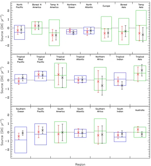
Fig. 3. Estimated fluxes and “total” uncertainty (GtC y−1) for the TransCom 3 (left) and total-76 (right) networks. The box shows the prior uncertainty, the horizontal bar the prior estimate. For each network the cross shows the predicted estimate and the error bar the one standard deviation total uncertainty.
each region in the “within-76” network in an attempt to ana-lyze the impact of this station. The largest contributions were made by the Tropical Africa and Temperate Eurasia regions. When we removed the IZO site from the network, the “tween” uncertainty reduced considerably, almost entirely be-cause of a reduction in the contribution from Tropical Africa. This is not simply related, as with the other sites, to the vari-ation in the response to this region at IZO. This is actually relatively small. However the overall constraint on this re-gion from the network is also small, leaving the inversion more succeptible to small model-model differences. It ap-pears that, while the variation in model response at a site is a reasonable guide to its influence on model-model differences in inversions, we must keep in mind the potential moderat-ing role of other sites. This highlights the risk of relymoderat-ing on single sites to constrain regions, consistent with the general findings of this study.
4 TransCom 3 comparison
In Section 3 we saw that the conclusion of Gurney et al. (2002), that new measurements would provide a useful con-straint on fluxes, was robust. We can also ask whether the particular flux distribution inferred in that paper was signif-icantly different from one with minimum total uncertainty. Figure 3 shows such a comparison. Comparing, first, the er-ror bars for both the optimal and TransCom 3 networks we notice relatively little reduction in total uncertainty. This is also evident from Table 2, which shows that the TransCom 3 network is nearly optimal with respect to total uncertainty. Note that, because the optimization is carried out for the globally summed uncertainty, there is no requirement that every region have its uncertainty reduced relative to the TransCom 3 case. Notwithstanding this, there are few re-gions where uncertainty is actually increased.
420 P. J. Rayner: Optimizing n etworks and model error Comparison of the predicted fluxes themselves also yields
only small differences between the two inverse calculations, especially if one normalizes the differences by the total un-certainty. This can be seen visually by considering the ovlap of the error bars for each region. In most cases the er-ror bars for each network include the central estimate for the other network. We should note that since the error bar rep-resents one standard deviation we should expect some esti-mates to differ at this level. There are four regions of appar-ently significant difference: the Southern Ocean, Australa-sia, the West Pacific and the Tropical Indian Ocean. Most of these are due to removal of specific stations between the TransCom 3 and total-76 networks, e.g. the anomalous Dar-win station. Sensitivity of the TransCom 3 inversion to this station has previously been noted by Law et al. (2003). One change is due to more systematic influences. The reduction of the Southern Ocean sink, already noted by Gurney et al. (2002), is strengthened in our optimal network. This occurs despite the great reduction in station density in this region. Roy et al. (2003) have noted that the reduction in Southern Ocean sink (relative to the prior) occurs even when almost all atmospheric observations are removed from the high south-ern latitudes. They conclude that the reduction in Southsouth-ern Ocean sink is required to match large-scale atmospheric con-centration gradients rather than particular local observations. The result of the present study suggests this result is also ro-bust to the choice of atmospheric transport model.
5 Conclusions
We have extended previous network optimization studies to include the impact of model-model variations in transport on inversion estimates. We find that network optimizations gen-erally choose quite small networks when optimizing only for the predicted uncertainty, concentrating on those sites that of-fer the strongest constraint. When model-model difof-ferences are considered, the optimization tries to average out some of the differences in transport by choosing more extensive networks, balancing the strength of constraint with the vari-ations in transport. For the network sizes considered here the optimization always wishes to use as many sites as possi-ble, confirming the conclusion of the TransCom 3 study that inversions are data not transport limited. We also find that the general distribution of fluxes predicted in that study is ro-bust to our minimum uncertainty metric, and that the network used in the TransCom 3 study is quite good under this metric. Finally we find that model-model variations in responses at a particular site are a reasonable predictor of the suitability of a site under this total uncertainty metric however this breaks down when regions are very poorly constrained.
Acknowledgements. The author wishes to thank R. Law and C.
Trudinger for helpful suggestions on the manuscript. The author also wishes to thank modellers who participated in the TransCom 3 project and the global CO2measurement community who provided
the various input data for this study.
Edited by: M. Heimann
References
Bousquet, P., Peylin, P., Ciais, P., Qu´er´e, C. L., Friedlingstein, P., and Tans, P. P.: Regional changes in carbon dioxide fluxes of land and oceans since 1980, Science, 290, 1342–1346, 2000. Denning, A. S., Holzer, M., Gurney, K. R., Heimann, M., Law,
R. M., Rayner, P. J., Fung, I. Y., Fan, S.-M., Taguchi, S., Friedlingstein, P., Balkanski, Y., Taylor, J., Maiss, M., and Levin, I.: Three-dimensional transport and concentration of SF6: A model intercomparison study (TransCom 2), Tellus, 51B, 266– 297, 1999.
GLOBALVIEW-CO2: Cooperative Atmospheric Data Integration
Project – Carbon Dioxide, CD-ROM, NOAA CMDL, Boulder, Colorado, (also available on Internet via anonymous FTP to ftp.cmdl.noaa.gov, path: ccg/co2/GLOBALVIEW), 2001. Gloor, M., Fan, S. M., Pacala, S., and Sarmiento, J.: Optimal
sam-pling of the atmosphere for purpose of inverse modeling: A model study, Global Biogeochem. Cycles, 14, 407–428, 2000. Gurney, K. R., Law, R. M., Denning, A. S., Rayner, P. J., Baker,
D., Bousquet, P., Bruhwiler, L., Chen, Y.-H., Ciais, P., Fan, S., Fung, I. Y., Gloor, M., Heimann, M., Higuchi, K., John, J., Maki, T., Maksyutov, S., Masarie, K., Peylin, P., Prather, M., Pak, B. C., Randerson, J., Sarmiento, J., Taguchi, S., Takahashi, T., and Yuen, C.-W.: Towards robust regional estimates of CO2
sources and sinks using atmospheric transport models, Nature, 415, 626–630, 2002.
Gurney, K. R., Law, R. M., Denning, A. S., Rayner, P. J., Baker, D., Bousquet, P., Bruhwiler, L., Chen, Y.-H., Ciais, P., Fan, S., Fung, I. Y., Gloor, M., Heimann, M., Higuchi, K., John, J., Kowalczyk, E., Maki, T., Maksyutov, S., Peylin, P., Prather, M., Pak, B. C., Sarmiento, J., Taguchi, S., Takahashi, T., and Yuen, C.-W.: TransCom 3 CO2 inversion intercomparison: 1.
Annual mean control results and sensitivity to transport and prior flux information, Tellus, 55B, 555–579, doi:10.1034/j.1600-0560.2003.00049.x, 2003.
Law, R. M., Rayner, P. J., Denning, A. S., Erickson, D., Fung, I. Y., Heimann, M., Piper, S. C., Ramonet, M., Taguchi, S., Tay-lor, J. A., Trudinger, C. M., and Watterson, I. G.: Variations in modelled atmospheric transport of carbon dioxide and the con-sequences for CO2inversions, Global Biogeochem. Cycles, 10,
783–796, 1996.
Law, R. M., Chen, Y.-H., Gurney, K. R., and TransCom 3 mod-ellers: TransCom 3 CO2inversion intercomparison: 2. Sensitiv-ity of annual mean results to data choices, Tellus, 55B, 580–595, doi:10.1034/j.1600-0560.2003.00053.x, 2003.
Patra, P. K. and Maksyutov, S.: Incremental approach to the optimal network design for CO2surface source inversion, Geophys. Res.
Lett., 29, 1459, doi:10.1029/2001GL013943, 2002.
Patra, P. K., Maksyutov, S., Baker, D., Bousquet, P., Bruhwiler, L., Chen, Y.-H., Ciais, P., Denning, A. S., Fan, S., Fung, I. Y., Gloor, M., Gurney, K. R., Heimann, M., Higuchi, K., John, J., Law,
R. M., Maki, T., Peylin, P., Prather, M., Pak, B., Rayner, P. J., Sarmiento, J. L., Taguchi, S., Takahashi, T., and Yuen, C.-W.: Sensitivity of optimal extension of CO2observation networks to model transport, Tellus B, 55, 498–511, 2003.
Rayner, P. J., Enting, I. G., and Trudinger, C. M.: Optimizing the CO2observing network for constraining sources and sinks,
Tel-lus, 48B, 433–444, 1996.
Rayner, P. J., Enting, I. G., Francey, R. J., and Langenfelds, R. L.: Reconstructing the recent carbon cycle from atmospheric CO2, δ13C and O2/N2observations, Tellus, 51B, 213–232, 1999.
R¨odenbeck, C., Houweling, S., Gloor, M., and Heimann, M.: Time-dependent atmospheric CO2inversions based on interannually
varying tracer transport, Tellus B, 55, 488–497, 2003.
Roy, T., Rayner, P., Matear, R., and Francey, R.: Southern hemisphere ocean CO2 uptake: reconciling atmospheric and
oceanic estimates, Tellus, 55B, 701–710, doi:10.1034/j.1600-0560.2003.00058.x, 2003.
Tans, P. P., Fung, I. Y., and Takahashi, T.,: Observational con-straints on the global atmospheric CO2 budget, Science, 247,