HAL Id: hal-03087686
https://hal.uca.fr/hal-03087686
Preprint submitted on 24 Dec 2020
HAL is a multi-disciplinary open access
archive for the deposit and dissemination of
sci-entific research documents, whether they are
pub-lished or not. The documents may come from
teaching and research institutions in France or
abroad, or from public or private research centers.
L’archive ouverte pluridisciplinaire HAL, est
destinée au dépôt et à la diffusion de documents
scientifiques de niveau recherche, publiés ou non,
émanant des établissements d’enseignement et de
recherche français ou étrangers, des laboratoires
publics ou privés.
Distributed under a Creative Commons Attribution| 4.0 International License
Scalable and Accurate Subsequence Transform
Michael Mbouopda
•, Engelbert Mephu
To cite this version:
Michael Mbouopda
•, Engelbert Mephu. Scalable and Accurate Subsequence Transform. 2021.
�hal-03087686�
Received: date / Accepted: date
Abstract Time series classification using phase-independent subsequences called shapelets is one of the best approaches in the state of the art. This approach is especially characterized by its interpretable property and its fast prediction time. However, given a dataset of n time series of length at most m, learning shapelets requires a computation time of O(n2m4) which is too high for practical datasets. In this paper, we exploit the fact that shapelets are shared by the members of the same class to propose the SAST (Scalable and Accurate Subsequence Transform) algorithm which is interpretable, accurate and more faster than the actual state of the art shapelet algorithm. The experiments we conducted on the UCR archive datasets shown that SAST is more accurate than the state of the art Shapelet Transform algorithm on many datasets, while being significantly more scalable. Keywords Time series · Classification · Shapelet · Scalability · Interpretability
1 Introduction
The world is surrounded today with data that change with time, these data are called time series and are exploited in many domains such as physic, chemistry, finance, medicine and industry. Many tasks can be performed on time series data and one of them is the classification task. Time series classification is a task that consists of learning a function able to classify objects represented as time series. This task has been successfully performed in astronomy in order to classify galaxies and stars (Moss, 2018; M¨oller and de Boissi`ere, 2020), in smart appliances in order to identify faults (Gupta et al., 2020), in medicine for rapid pathogen identification
Michael Franklin MBOUODPA
Clermont Auvergne University, CNRS, ENSMSE, LIMOS, F-63000 CLERMONT-FERRAND, FRANCE
E-mail: michael.mbouopda@uca.fr Engelbert MEPHU NGUIFO
Clermont Auvergne University, CNRS, ENSMSE, LIMOS, F-63000 CLERMONT-FERRAND, FRANCE
(Papagiannopoulou et al., 2019), in satellite image analysis (Sanchez et al., 2019) and in many other applications.
Nowadays, there are many accurate methods for the classification of time se-ries (Bagnall et al., 2017). Depending of the feature used for classification, these methods are grouped in six categories (Hills et al., 2014):
– whole series: these methods use the whole series as feature. The main idea is to define a similarity distance (Euclidean distance, Dynamic Time Warping and its variants, Time Warped Edit Distance, etc) between time series and then use the nearest neighbor algorithm for classification. The Fast Ensemble of Elastic Distance or FastEE (Tan et al., 2020) is an ensemble method that combines different similarity distances.
– interval : the discriminative features are localized at some specific intervals on the time series, and are computed using some aggregate functions (mean, median, max, etc). A supervised classifier is then trained on the computed features. Time Series Forest or TSF (Deng et al., 2013) is to our knowledge the most popular and the state of the art algorithm in this category. Recently, the Supervised Time Series Forest or STSF has been proposed (Cabello et al., 2020). It uses a supervised approach to learn the best intervals.
– shapelet : shapelet-based methods (Ye and Keogh, 2009; Rakthanmanon and Keogh, 2013; Hills et al., 2014) use phase independent patterns (subsequences) as features. These subsequences are shared by members of the same class and are called shapelets. An instance is classified regarding the shapelets it contains. – dictionary : these methods are used when the classes have the same discrimi-native patterns, however at different frequencies for each class. Generally, the time series are converted to sequences of symbols before extracting patterns also called words. The Bag of Symbolic-Fourier Approximation Symbols or simply BOSS (Sch¨afer, 2015) and its variants the Contract BOSS (Middle-hurst et al., 2019) and the Spatial BOSS (Large et al., 2019) are some state of the art algorithms in this category. Another state of the art is the Word Ex-trAction for time SEries cLassification or WEASEL (Sch¨afer and Leser, 2017) algorithm. Recently, BOSS and WEASEL have been used in the early time series classification framework called TEASER (Sch¨afer and Leser, 2020). – spectral : these methods work in the frequency domain and are able to extract
features that are very hard to find in the time domain. Some popular techniques used here are power spectrum and auto correlation function (ACF) (Corduas and Piccolo, 2008; Bagnall and Janacek, 2014; Flynn et al., 2019).
– hybrid : these are methods that work on different features at the same time in order to take advantage of each type of feature. The most famous model in this category is HIVE-COTE (Lines et al., 2018) which is composed of 5 com-ponents, each focusing on one type of features (whole series, interval, shapelet, dictionary or spectral) and is an ensemble of classifiers. TS-CHIEF (Shifaz et al., 2020) is a tree-based hybrid method that uses all the previous features except shapelet. A recent method is ROCKET (Dempster et al., 2020) which uses randomly generated convolutional kernels in order to extract different types of features.
Recently, deep learning has shown its effectiveness in many tasks, including time series classification (Fawaz et al., 2019). Some state of the art deep learning
of the longest time series. This high time complexity is due to the large number of shapelet candidates that need to be evaluated in order to find the top best shapelets.
A human brain is able to recognize a lot of variations of an object after see-ing a ssee-ingle variation. For instance, we are able to recognize any model of car after seeing one of them, we can recognize many species of dog if we have ever seen a dog. This ability is called core object recognition (DiCarlo et al., 2012). Inspired by this amazing behavior of our brain, we claim that a shapelet model should be able to recognize any variation of a shapelet if it knows one or a few number of its variations. Simply defined, a shapelet is a pattern that is shared by the time series that belong to the same class. Therefore, any single instance of a class should contain all the shapelet candidates for that class. Guided by this observation, we propose the Scalable and Accurate Subsequence Transform (SAST) algorithm, a time series classification algorithm that is accurate, scalable and whose predictions are interpretable. Existing shapelet based methods use the whole dataset to generate shapelet candidates, then use information gain to select the top best shapelets before doing the classification using a supervised classifier. SAST proceeds differently by using only a single instance per class in order to generate shapelet candidates. Furthermore, shapelet candidates are not assessed beforehand of classification. The supervised classifier automatically identified the top best shapelets during its training phase. The key points of our contribution are the following:
– We propose a new design of shapelet based classification of time series. The proposed design allows us to build a scalable and accurate shapelet method for the classification of time series. In particular, our method took 1 second to classify the Chinatown dataset with an accuracy of 96%, while the state of the art shapelet based algorithm (Shapelet Transform Classifier) took 51 seconds and achieved an accuracy of 97% on the same computer.
– We give a public implementation of our model that is compatible with the well known scikit-learn machine learning library. This allows anyone to easily use our model on its own data, and also to reproduce our experiments.
The rest of this paper is organized as follows: we start by setting the background and present related work in Section 2. In Section 3 we describe our proposed method SAST and the idea behind. Our experiments are described in Section 4, Section 5 summarizes this work and presents future steps.
2 Background and related work
The building blocks of shapelet based methods for time series classification are subsequence, similarity measure and of course the notion of shapelet. So, we start by defining these terms.
Definition 1 (Time series) A sequence of n real values recorded in time. n is the length of the time series
T = (t1, t2, ..., tn) (1)
A time series can be decomposed in subsequences of different lengths.
Definition 2 (Subsequence or pattern) Given a time series T of length n, a subsequence (also called pattern) S of length l is a sequence of l consecutive values of T starting at time step j.
S = (s1, s2, ..., sl) = (tj, tj+1, ..., tj+l−1) (2)
Two subsequences are said similar if the distance between them is less than a predefined threshold. Euclidean distance and Dynamic Time Warping (DTW) are the most used similarity distance in time series classification (Bagnall et al., 2017). For shapelet based methods, Euclidean distance is preferred in the literature (Ye and Keogh, 2009; Bagnall et al., 2017) and we also use it in this work. However, any distance can be used to compute the similarity between subsequences.
A time series is similar to a pattern if there is a subsequence of that time series that is similar to the pattern. Formally, the similarity between a time series T of length m and a subsequence S of length l is defined as follows:
dist(T, S) = min ∀R∈Wl({ l X i=1 (ri− si)2}) (3)
In the previous equation, Wlis the set of all subsequences of length l contained in the time series T . The patterns S and R are put on the same scale before the distance computation using a normalization technique. Beware that we are not using the Euclidean distance, but the square of the Euclidean distance. As a matter of fact, the square root can be seen as a change of the similarity’s scale.
Among all the patterns contained in a time series dataset, some can be used as discriminative features in order to find the class label of an unseen time series. These patterns are called shapelets. Shapelet has been introduced as a primitive for time series classification by Ye and Keogh (2009). The authors proposed a shapelet based decision tree in which each node is a subsequence and the time series arriving at a node are split in two groups such that one group contains data that are similar to the subsequence at that node, and the other group is the set of data that are not similar to the subsequence. Fig. 1 illustrates a node in the proposed decision tree.
The subsequence used at a node of the tree is chosen such that the information gain (IG) is maximized (Ye and Keogh, 2009; Hills et al., 2014).
time series with their class labels ci taken from a finite set of classes C, a shapelet S? is a subsequence that maximizes the information gain
S? = argmax S∈W
IG(D, S) (4)
In Eq. 4, W is the set of all subsequences in the dataset. For a time series of length m, there are m − l + 1 subsequences of length l and m(m+1)2 subsequences in total for a single time series. Since any subsequence in the dataset is a shapelet candidate, and there are about O(nm2) subsequences, evaluating them is very time consuming. Because of that, the time complexity of the shapelet decision tree algorithm is n2m4. Hence, the method does not scale well.
Many works have been proposed in order to improve the scalability, but at the cost of accuracy and possibly interpretability. Fast shapelet (Rakthanmanon and Keogh, 2013) reduces the time complexity to O(nm2) by using a symbolic representation of time series. Symbolic representations have the benefit of reducing the time series length. Other authors proposed to reduce the space of shapelet candidates by randomly pick a fraction of subsequences to be evaluated (Renard et al., 2015; Wistuba et al., 2015; Karlsson et al., 2016).
The state of the art algorithm for shapelet based classification of time series is the Shapelet Transform (STC) algorithm (Hills et al., 2014; Bostrom and Bag-nall, 2015). This algorithm designs shapelet based classification as a three steps process. The first step is the selection of the top k shapelets. The second step is the shapelet transformation where each time series in the dataset is replaced by a vector of its distances to each of the selected shapelets. The final step consists of training a supervised classifier on the transformed dataset. Although the time complexity of this algorithm is still n2m4, it is the shapelet based algorithm that obtains the best classification accuracy (Bagnall et al., 2017). Early abandon tech-niques and shapelet candidates pruning have also been used in order to reduce the running time of shapelet based algorithms (Ye and Keogh, 2009; Rakthanmanon and Keogh, 2013; Hills et al., 2014).
STC is not the most accurate time series classification algorithm in the liter-ature, there exists other models that are more accurate, but they are less inter-pretable. The current state of the art methods for time series classification are HIVE-COTE (Lines et al., 2018), TS-CHIEF (Shifaz et al., 2020) and ROCKET (Dempster et al., 2020). The time complexity of HIVE-COTE is bounded by the complexity of its shapelet component, that is n2m4. Therefore decreasing the com-putation time of the shapelet component will make HIVE-COTE more efficient in terms of running time. TS-CHIEF is a forest of trees in which a time series
follows a branch if it is closer to the reference time series (there is one reference time series for each class) associated with that branch than to the reference time series of other branches. TS-CHIEF does not use shapelet features because of the time complexity needed for their computation. ROCKET is the most scalable state of the art method, it is based on random convolutional kernels that are used to transform the dataset. ROCKET results are not easily interpretable because the kernels used are short, independent and not sample from the dataset.
ROCKET is architecturally similar to SAST, our proposal described in the next section. However the way both models work is different in two folds: firstly, the subsequences (convolutional kernels in ROCKET) are the subsequences of some reference time series randomly chosen from the dataset, and hence they are dependent and have variable lengths. Secondly, SAST does not use the convolution operator as similarity measure, but the Euclidean distance. These properties of SAST are the reasons of its scalability and interpretability. SAST is a scalable and accurate alternative to STC. It can be used to reduce the computation time of shapelet module in HIVE-COTE, and can be integrated to TS-CHIEF at the cost of little computation time. We believe that adding shapelet features in TS-CHIEF could increase its accuracy.
3 SAST: Scalable and Accurate Subsequence Transform
In time series classification, a shapelet is ideally a pattern that is shared by every instances of the same class, and that instances of other classes do not have, they are called discriminative patterns or subsequences. The number of patterns in a dataset of n time series of length m is O(nm2), and state of the art shapelet algorithms must evaluate each of them by computing their information gain. Reducing this number will make shapelet models faster to train. In this section we propose a way to reduce the number of shapelet candidates. Then we show that there is no need to select the top best shapelets beforehand. Finally we present a novel method for shapelet based time series classification.
3.1 Reducing the number of shapelet candidates
Human brain effortlessly performs core object recognition, the ability to recognize objects despite substantial appearance variation (DiCarlo et al., 2012). This gives human the capability to recognize a vast number of objects that have the same name just by seeing a few of them. Heeger (2002-2014) used Fig. 2 in his lecture notes on Perception to illustrate the notion of invariance in recognition. This figure shows different ducks. Some are in water while others are not, some ducks are photographs and other are drawings. Despite all this variability, a human brain that has already seen a duck is able to recognize that each object on this figure is a duck.
A shapelet is a pattern, a shape that is “common” to time series that have the same class label. By “common”, we do not mean that these time series have exactly that shapelet, but they have a pattern that is very similar to the shapelet. Any pattern that is similar to a shapelet can be considered as a variation of that shapelet. Therefore, we introduce the core shapelet recognition task, which goal
Fig. 2: Illustration of invariance in recognition.
is to recognize any variation of a shapelet by just seeing one or very few number of its variations. We argue that time series classification based on shapelets is a core shapelet recognition task and that it should be solved using very few shapelet candidates than it has been done since the introduction of shapelets by Ye and Keogh (2009). Hence, instead of generating shapelet candidates from the whole dataset, we propose to use only one or a few number of instances per class. In this way, the learning algorithm must focus on one (or a few number) variation of each shapelet candidate to classify a time series. We acknowledge that the more variations the model learns, the more accurate the model will be. However this can also cause the model to overfit, especially when the training data is not enough representative of the testing data.
In Fig. 3, we have three randomly selected instances of the Chinatown dataset from the UEA & UCR archive (Anthony Bagnall and Keogh, 2018). This dataset has two classes of data. The left example is from class 1 and the second example (in the middle) is from class 2. It is easy to observe that the instance from class 1 starts by a deep valley, while the instance of class 2 does not. One reason that can be considered in order to classify the instance on the right in class 2 is that it does not start by a valley. Hence, observing only one instance per class can be enough to discover discriminative patterns and successfully perform classification of new instances.
Fig. 3: Three randomly selected instances from the Chinatown dataset. The in-stance on the right is probably from class 2 since it does not start with a valley
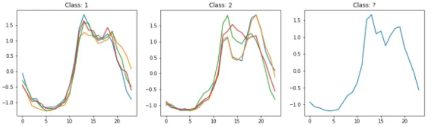
Fig. 4 shows 4 randomly selected instances for each class. Instances of the same class are superposed in order to expose global patterns. The figure emphasizes the previous observation that class 1 contains instances that start by a deep valley while class 2 are instances that are more flat at the beginning.
Fig. 4: Some randomly selected instances from the Chinatown dataset. The in-stance on the right is definitely from class 2
Based on this observation, we propose the following theorem:
Theorem 1 Let D = {(T1, c1), (T2, c2), ..., (Tn, cn)} be a dataset of time series. Let Dc be any subset of D that contains at most k (k ≥ 1) instances from each class. If classes in D can be distinguished using shapelets, then for any shapelet shp of D, there exists a time series in Dc that is similar to shp.
Proof Let’s assume that classes in D are distinguishable using shapelets and that there exists a shapelet shp for the dataset D that is not similar to any time series in the set Dc. Since Dc contains at least a time series of each class in D, any shapelet for the dataset D must be similar to at least one time series in Dc. It follows from there that assuming shp to be a shapelet is wrong. Therefore the theorem is true.
From the previous theorem, any shapelet shp of D is always similar to a pattern in Dc. Therefore, a shapelet algorithm that generated shapelet candidates from Dc can achieve the same accuracy as if D was used. We run the shapelet transform algorithm (STC) (Hills et al., 2014) on the Chinatown dataset and plotted the top 5 shapelets that have been selected for each class in Fig. 5. The shapelets on the first row clearly identify the valley at the beginning of time series in class 1. Although they are coming from different time series, they are very similar in shape. Likewise, the shapelets on the last row identify the flat starting of instances in class 2. Generating shapelet candidates from the whole dataset makes STC learn different variations of the same patterns.
Applying theorem 1 in the STC algorithm reduces the number of shapelet candidates from O(nm2) to O(ckm2), where c is the number of classes in the dataset. In particular, with k = 1, the modified STC model took about 10 seconds to classify the Chinatown dataset with an accuracy of 96% (average over five runs), while the original STC algorithm took 72 seconds and gave an accuracy of 97% on the same computer. Therefore, the modified STC algorithm is about 7 times faster and achieves almost the same accuracy as the original algorithm. The extracted
Fig. 5: Top 5 shapelets extracted for each class of the Chinatown dataset by the shapelet transform algorithm.
shapelets are shown in Fig. 6. Different variations of the same shapelet are not learnt anymore. For this dataset, exactly one shapelet has been selected for each class. We assessed how the value of k affects the STC’s accuracy and computation time for different datasets and the results are given in Appendix B.
Fig. 6: Shapelets extracted by STC on the Chinatown dataset using a single ran-domly selected instance per class to generate shapelet candidates.
3.2 Identify shapelets using feature importance analysis
When time series classification using shapelets was introduced, shapelets were learnt while building a decision tree (Ye and Keogh, 2009). Later, shapelet trans-form (STC) (Hills et al., 2014) has been proposed to allow the use of any super-vised classifier. The algorithm proceeds by finding the top best shapelets, then transforms the dataset using the found shapelets and finally trains a classifier on the transform dataset (Hills et al., 2014; Bostrom and Bagnall, 2015; Karlsson et al., 2016). Therefore, there are three main steps: feature extraction where best
shapelets are selected, dataset transformation where each time series is replaced by a vector of its distance to the selected shapelets and finally training where a classifier is trained on the transformed dataset.
We propose to remove the feature extraction step and use every shapelet can-didates to transform the dataset. After training the classifier on the transformed dataset, a post hoc method for model explanation can be used to find the most important features. The importance of a feature represents how much that feature is correlated to the target variable (Dash and Liu, 1997; Molnar, 2020).
Theorem 2 Let D = {(T1, c1), (T2, c2), ..., (Tn, cn)} be a dataset of time series, and S the set of all subsequences in D. Let Df = {(x1, c1), (x2, c2), ..., (xn, cn)} be a dataset such that xi = [xi:1, xi:2, ..., xi:|S|], where xi:j = dist(Ti, Sj). If the jth feature is an important feature given by the analysis of feature importance for the dataset Df, then Sj is a shapelet for the dataset D.
Proof Let’s suppose the jth feature is an important feature, and that Sj is not a shapelet for the dataset. By definition 3, not being a shapelet means that the information gain of Sjis not high enough, and whether a time series T is similar or not to Sjdoes not give any clue about the class of T . Therefore, knowing dist(T, Sj) doesn’t help to classify T . In other words, the jthfeature is not correlated to the target variable. Hence, it cannot be an important feature. This proves the theorem. The importance of a feature in a tree based algorithm determines how much it reduces the variance of the data compared to the parent node (Dash and Liu, 1997; Molnar, 2020). This corresponds exactly to the definition of a shapelet (see Def. 3). In a linear model, the absolute value of the weight of an important feature will be greater than the one of a less important feature (Molnar, 2020). Classifiers such as decision trees and linear models are said to be inherently interpretable since a post hoc analysis is not required to interpret their predictions. More generally, when a classifier is fitted, a post hoc explainer can be used to find most important features (Murdoch et al., 2019) in order to interpret predictions. Two examples of these post hoc explainers are LIME (Ribeiro et al., 2016) and SmoothGrad (Smilkov et al., 2017) for saliency maps. More methods can be found in the review of Samek et al. (2020). Hence, selecting shapelets beforehand of classification using information gain can be skipped, since the classifier can automatically learn the top best shapelets during its training iterations.
3.3 Time series classification with SAST
Time series classification with SAST (Scalable and Acurate Subsequence Trans-form) is designed with respect to Proposition 1 and Proposition 2. A visual view of the the method is shown in Fig 7. There are two main blocks:
– The classification block: this block is actually the SAST algorithm and begins with the random selection of reference time series from which subsequences are then generated. Thereafter, the dataset is transformed by replacing each time series with a vector of its distances to each subsequence. Finally a supervised classifier (illustrated here by a decision tree) is trained on the transformed dataset.
Fig. 7: Visual view of the SAST method
A pseudo code of the SAST algorithm is given by Algorithm 1. SAST takes as input the time series dataset D, the number k of instances to randomly select from each class in order to create the shapelet candidates, the list of lengths to use to generate shapelet candidates, and finally the supervised classifier C that is going to be trained on the transformed dataset.
Algorithm 1: ScalableAndAccurateSubsequenceTransform
Input: D = {(T1, c1), (T2, c2), ..., (Tn, cn)}, k: the number of instances to use per
class, length list: the list of subsequence lengths, C: the classifier to use
1 begin
/* randomly select k instances per class from the dataset */
2 Dc← randomlySelectInstancesP erClass(D, k)
/* generate every patterns of length in length list from Dc */ 3 S ← generateShapeletCandidates(Dc, length list)
/* transformed the dataset using every patterns in S */
4 Df ← ∅ 5 for i ← 1 to n do 6 xi← [] 7 for j ← 1 to |S| do 8 xi[j] ← dist(Ti, Sj) 9 end 10 Df← Df∪ {(xi, ci)} 11 end
/* train the classifier on the transformed dataset */
12 clf ← trainClassif ier(C, Df)
13 return (clf , S) ; // the trained classifier and the shapelet candidates
SAST starts by randomly select k instances per class from the dataset (line 2). By default, k is set to one. We call the selected instances reference time series. The next step is the generation of every subsequences of length in length list from the reference time series (line 3). The dataset transformation is performed from line 4 to 11. Here, the similarity between each time series in the dataset and each shapelet candidate is computed. The classifier taken as input is then trained on the transformed dataset (line 12). The algorithm returns the trained classifier, the shapelet candidates that have been generated.
After the training is done, the class labels of a test dataset can be predicted in two steps: firstly the dataset is transformed using the shapelet candidates that have been generated during training, and finally the trained classifier is used to predict the class labels of the transformed test dataset.
3.4 SAST time complexity
Each step of the SAST algorithm runs in a finite amount of time, therefore the algo-rithm always terminates. Selecting k reference time series is done in O(c) time com-plexity, c is the number of classes in the dataset. There are m−l+1 subsequences of length l in a time series of length m. The total number of subsequences for a time series ism(m+1)2 . Since there are kc reference time series in a dataset with c classes, generating all shapelet candidates is done in O(kcm2). The transformation step re-quires O(nm2) distance computations, each of which requires O(l) (l is the length of the subsequence) point wise operations. As the maximum subsequence length is m, the time complexity of the transformation step is O(nm3). Therefore, to total time complexity of SAST is O(c) + O(kcm2) + O(nm3) + O(classif ier), where O(classif ier) is the time complicity of the classifier used. The overall asymptotic time complexity of the SAST algorithm is therefore O(nm3)+O(classif ier). SAST is much faster than the state of the art shapelet transform algorithm (Hills et al., 2014) whose time complexity is O(n2m4) + O(classif ier),
3.5 Ensemble of SAST models
SAST accuracy is highly dependent on the randomly selected reference series. If a reference time series is noisy or not representative of its class, then it could be difficult for SAST to learn best shapelets for the dataset. Furthermore, the random selection of reference time series could lead to a variance in performance. We use Bagging (Breiman, 1996) to leverage these possible issues and we call the obtained model SASTEnsemble (or SASTEN in reduced form). SASTEN is obtained by ensembling r SAST models. Each individual model in the ensemble uses randomly selected reference time series and may also have different parameters, especially parameter controlling the length of shapelet candidates (that is length list in Algo. 1). The final prediction is obtained by averaging the predictions of every SAST models in the ensemble.
on some datasets in Appendix C. We use two classifiers available in scikit-learn: – Random Forest (RF): all features are evaluated at each node to find the best
split and a split is selected if the impurity decreases by about 0.05. These prop-erties are ensured by the parameters max features and min impurity decrease respectively.
– Ridge Classifier with LOO: this is the ridge classifier with built-in Leave-One-Out cross validation. The cross validation is used to select the best regulariza-tion parameter between 10 log spaced values ranging from −3 to 3.
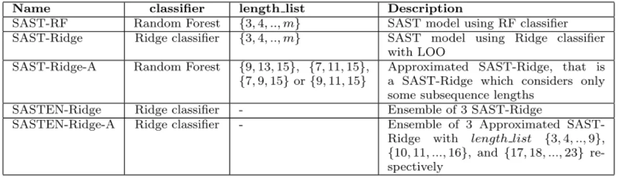
Table 1 describes the models that we use in our experiments. We compare our models especially to the shapelet transform algorithm STC (Hills et al., 2014), which is to our knowledge the state of the art shapelet based method. We also compare SAST to other state of the art algorithms that are not necessarily based on shapelet: ROCKET (Dempster et al., 2020), HIVE-COTE (Lines et al., 2018), Catch22 (Lubba et al., 2019) and BOSS (Sch¨afer, 2015). The results of these models are taken from the UEA & UCR repository (Anthony Bagnall and Keogh, 2018).
Name classifier length list Description
SAST-RF Random Forest {3, 4, .., m} SAST model using RF classifier SAST-Ridge Ridge classifier {3, 4, .., m} SAST model using Ridge classifier
with LOO SAST-Ridge-A Random Forest {9, 13, 15}, {7, 11, 15},
{7, 9, 15} or {9, 11, 15}
Approximated SAST-Ridge, that is a SAST-Ridge which considers only some subsequence lengths
SASTEN-Ridge Ridge classifier - Ensemble of 3 SAST-Ridge
SASTEN-Ridge-A Ridge classifier - Ensemble of 3 Approximated
SAST-Ridge with length list {3, 4, .., 9}, {10, 11, ..., 16}, and {17, 18, ..., 23} re-spectively
Table 1: List of models used in our experiments
We experiment using 39 randomly selected datasets from the UEA & UCR repository (Anthony Bagnall and Keogh, 2018). The datasets in the repository are different in terms of series length, number of series, number of classes and application domain. Each dataset is already split into train and test sets. There are 128 datasets on the repository, but we are limited by the computation power
and the time constrain on our computing clusters. However, we plan to extend our experiments on the remaining datasets in near future.
4.1 Accuracy
Fig. 9 shows a pairwise comparison of SAST-Ridge to other models. The first thing to note is that SAST-Ridge is generally more accurate than SAST-RF on our datasets (Fig. 9a). This is why we use SAST-Ridge as the pivot in our comparison. We tried several length list for the approximated SAST model, and we are presenting here only the four that achieved the best accuracy on our datasets. The critical difference diagram between these four models is given in Fig. 8. There is no significant difference between the models, however the model us-ing length list = {7, 11, 15} is the best of all. When not clearly precised in the rest of this paper, SAST-Ridge-A is the approximated SAST-Ridge model with length list = {7, 11, 15}.
Fig. 8: Critical difference diagram between approximated SAST models
4.1.1 Comparison to STC
In this part, we start by assessing the performance of SAST, SASTEN and their approximated variants before comparing our models to STC.
The approximated SAST-Ridge is less accurate than SAST-Ridge in general (Fig. 9b). However it is important to note that the approximated model wins on 9 datasets. Therefore, knowing a prior about possible shapelet lengths can be used to train the model faster and without losing accuracy. Furthermore, ensembling approximated SAST models, each one focusing on different shapelet lengths is a possible way to improve accuracy while decreasing the computation time. In fact, SASTEN-Ridge-A is more accurate than SAST-Ridge on 20 datasets and less accurate on 18 (Fig. 9c).
Fig. 9d reveals that ensembling SAST-Ridge models improves accuracy on almost every dataset. But the improvement is slight, because even though the reference time series are chosen randomly, SAST-Ridge has very low variance in accuracy over multiple runs.
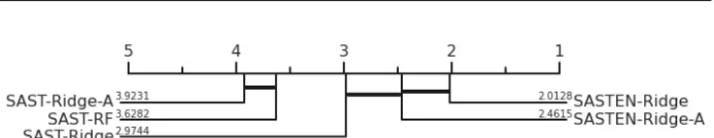
The critical difference diagram between SAST models is shown in Fig. 10. SASTEN-Ridge is the best of all, follows by SASTEN-Ridge-A which is not signif-icantly less accurate. SAST-Ridge is the third best model and is not signifsignif-icantly worse than Ridge-A, but is considerably less accurate than SASTEN-Ridge. SAST-Ridge-A and SAST-RF are significantly less accurate.
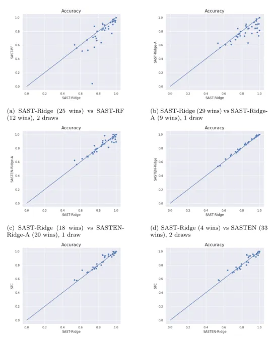
(a) SAST-Ridge (25 wins) vs SAST-RF (12 wins), 2 draws
(b) SAST-Ridge (29 wins) vs SAST-Ridge-A (9 wins), 1 draw
(c) SAST-Ridge (18 wins) vs SASTEN-Ridge-A (20 wins), 1 draw
(d) SAST-Ridge (4 wins) vs SASTEN (33 wins), 2 draws
(e) SAST-Ridge (12 wins) vs STC (26 wins), 1 draw
(f) SASTEN-Ridge (18 wins) vs STC (18 wins), 1 draw
Fig. 9: Pairwise comparison of models’ accuracies
STC, the state of the art shapelet method to our knowledge is more accurate on more datasets than our model SAST-Ridge (Fig. 9e). SAST-Ridge is better on 12 datasets, worse on 26 and there is one draw. The difference in accuracy is not too large between both models. However, Fig. 9f shows that SASTEN-Ridge, the
Fig. 10: Critical difference diagram between SAST models
ensemble of 3 SAST-Ridge is as accurate as STC with 18 wins each and a draw. Elsewhere, as shown in Appendix C, using more reference time series will improve the accuracy of our models.
4.1.2 Comparison to others
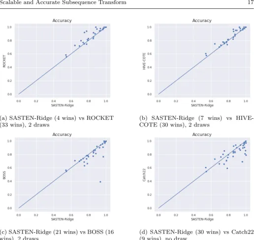
In Fig. 11, we compare SASTEN-Ridge to the state of the art models Catch22, BOSS, ROCKET and HIVE-COTE.
SASTEN-Ridge largely outperforms Catch22 and BOSS. Fig. 11c shows the accuracy of BOSS and SASTEN-Ridge. Our model wins on 21 datasets, loses on 16 datasets and there are 2 draws. Furthermore, our model largely outperforms BOSS on the SmoothSpace dataset. In fact, SASTEN-Ridge achieves an accuracy of 93% whereas BOSS achieves only 39%. SASTEN-Ridge is also more accurate than Catch22 with 30 wins versus 9 losses (Fig. 11d).
To the best of our knowledge ROCKET and HIVE-COTE are the most ac-curate time series classifiers. Although our model uses only shapelet features, it manages to outperform ROCKET and HIVE-COTE on some datasets (Fig. 11b and 11a)
The critical difference diagram in Fig. 12 shows how our models are ranked regarding five state of the art time series classifiers, including STC, the model which we want to improve scalability. The cliques on the figure are:
– SASTEN-Ridge-A, SAST-Ridge, BOSS, Catch22 – SASTEN-Ridge-A, SAST-Ridge, BOSS, STC
– SASTEN-Ridge-A, SAST-Ridge, HIVE-COTE, ROCKET – SASTEN-Ridge-A, SASTEN-Ridge, BOSS, Catch22 – SASTEN-Ridge-A, SASTEN-Ridge, BOSS, STC
– SASTEN-Ridge-A, SASTEN-Ridge, HIVE-COTE, ROCKET
Hence, in average SASTEN-Ridge-A is better than BOSS and Catch22. In ad-dition, SASTEN-Ridge is considerably more accurate than Catch22. HIVE-COTE and ROCKET are not significantly better than our ensemble model SASTEN-Ridge nor SASTEN-SASTEN-Ridge-A. The most important thing here is that none of our models is significantly less accurate than STC. Particularly, SASTEN-Ridge and STC are ranked almost the same. However, we show in Section 4.2 that our models are much more scalable than STC.
(a) SASTEN-Ridge (4 wins) vs ROCKET (33 wins), 2 draws
(b) SASTEN-Ridge (7 wins) vs HIVE-COTE (30 wins), 2 draws
(c) SASTEN-Ridge (21 wins) vs BOSS (16 wins), 2 draws
(d) SASTEN-Ridge (30 wins) vs Catch22 (9 wins), no draw
Fig. 11: SASTEN-Ridge-A vs state of the art time series classifiers
Fig. 12: Critical difference diagram SASTEN-Ridge-A vs state of the art
4.2 Scalability
The scalability of SAST is assessed regarding two criteria: the time series length and the number of time series in the training set. In this experiment, SAST with Ridge classifier is used, and we removed the word Ridge from models’ names.
(a) Regarding time series length (b) Regarding the number of time series
Fig. 13: Running time (in second) of each model
4.2.1 Time series length
Here we use the dataset HouseTwenty from the UCR repository (Anthony Bagnall and Keogh, 2018). It is a binary dataset of electricity usage in houses. The training set has 34 time series and of length 3000 each. We vary the series length starting at 32 and only the first time steps up to the current length are used to train our models. The running time of each model is given in Fig. 13a.
For each of the four models, the training time increases with the length of time series in the dataset. However, SAST models are much more scalable than STC, and SASTEN-A is the most scalable of all, since it uses a fixed number of shapelet candidates whatever the length of time series. For SASTEN-A, increasing the length of the time series only increases the computation time of the similarity between time series and shapelet candidates. More specifically, STC takes about 1 hour and 40 minutes to train on a dataset of 34 time series of length 64, while SAST, SASTEN and SASTEN-A take about 13 seconds, 27 seconds and 8 seconds respectively. For the same number of time series but now of length 256, STC takes a bit more than a day, while SAST, SASTEN and SASTEN-A take about 14 minutes, 26 minutes and 2 minute respectively. Therefore, even our slowest method SASTEN is 55 times faster than STC. SASTEN-A and SAST are respectively 1440 times and 102 times faster than STC.
4.2.2 Training set size
The Chinatown dataset is used here. It is a binary dataset with time series of length 24. There are 20 instances in the training set and we use random oversampling to create bigger versions of this dataset. Fig. 13b shows the running time of each models.
The training time of each model increases near linearly with the number of time series in the dataset. STC’s training time starts higher and increases much faster compared to other models. This is not surprising since the training time of shapelet methods is extremely related to the number of shapelet candidates, and the number of shapelet candidates in STC increases with the number of time series while the number of shapelet candidates in a SAST model increases with the number of classes. More precisely, STC takes about 12 minutes on a dataset
didate extracted from a time series whose class label is known. Shapelet candidates related to the most important features are the top best shapelets. We say that any shapelet candidate is from the class of the time series from which it has been ex-tracted. Therefore, the class label of a time series can be interpreted by looking at the class labels of the shapelet candidates to which it is the most similar. Let us interpret the predictions of SAST-RF and SAST-Ridge trained on the Chinatown dataset. Although feature importance are computed differently for both models, we show that their predictions are interpretable in the same manner.
Fig. 14 and 15 show the top 5 best shapelets plotted on the reference time series for the Chinatown dataset with respect to SAST-Ridge and SAST-RF respectively. The top rows of the figures are the reference time series selected from class 1, while the second rows are the reference time series selected from class 2. A perfect match between a shapelet candidate and a reference time series means that the shapelet has been extracted from that reference time series. Hence, the top 5 best shapelets learnt by SAST-Ridge are from class 1. The second of the top 5 best shapelets learnt by SAST-RF is from class 1, while the four others are from class 2.
Fig. 14: Top 5 shapelets learnt by SAST-Ridge on Chinatown.
In order to predict the class label of a test time series, SAST identifies the most important features similar to the time series. In other words, SAST checks if the time series contains subsequences that are similar to the most important features. Fig. 16 shows the matches between the top 5 most important features learnt by SAST-Ridge and two randomly selected test time series. We can note that
Fig. 15: Top 5 shapelets learnt by SAST-RF on Chinatown.
the model correctly predicts the class labels. Since the top 5 shapelets learnt by SAST-Ridge are from class 1, there are near perfect matches with the test instance from class 1 (see Fig. 16 top). A near perfect match between a subsequence and shapelet candidate means that the subsequence is a variation of that shapelet candidate. No good match is found with the test instance from class 2 (see Fig. 16 bottom). Therefore, we have an explanation of why the first instance is predicted as coming from class 1, while the second one is predicted as coming from class 2. The same analysis is shown for RF in Fig. 17. Like Ridge, SAST-RF also predicted the class labels correctly. The first test time series has a near perfect match with the second top best shapelet candidate (see Fig. 17 top) which is a shapelet candidate of class 1. The other top best shapelet candidates, which are all from class 2 do not match with the first time series. This explains why the predicted class label for the first time series is class 1 and not class 2. The first, third, fourth and fifth top best shapelet candidates, which are all from class 2 have near perfect matches with the second time series, while the second top best shapelet candidate, which is from class 1 does not match (see Fig. 17 bottom). Hence, we can interpret why the class label of the second instance is predicted as class 2 and not class 1.
Therefore, we experimentally proved in this Section that RF and SAST-Ridge automatically learn to put more attention on the subsequences that are shapelets for the considered dataset. More generally a SAST model automatically learns to put more attention on shapelet candidates that are shapelets during its training. It also automatically learns to put less attention on the shapelet candidates that are not shapelets. We also note that the top best shapelets learnt by SAST-Ridge and SAST-RF on the Chinatown dataset are the same as the one selected by STC (see Fig. 5).
5 Conclusion
In this work, we shown that the number of shapelet candidates in a shapelet algorithm can be reduced considerably without losing accuracy. We also shown that it is not always necessary to learn shapelets beforehand of classification. We
Fig. 16: Explanation of SAST-Ridge predictions on two random test instances
Fig. 17: Explanation of SAST-RF predictions on two test instances
introduced the Scalable and Accurate Subsequence Transform (SAST) algorithm which is interpretable, accurate and a more scalable alternative to the Shapelet Transform algorithm. Our experiments revealed that a good trade-off between accuracy and scalability can be found by ensembling different SAST models, each one focusing on different shapelet candidates.
We plan to do many improvements on the SAST algorithm in the future. Particularly, we will speed up the distance computation by using lower bounding and early abandon techniques. Then we will prune similar subsequences in order to further reduce the number of shapelet candidates.
Although we focused on time series classification in this paper, we hope that the same idea can be used in the near future to increase the scalability of shapelet-based time series clustering, especially when a high time complexity distance like FOTS (Siyou et al., 2020) is used.
Acknowledgements This work is funded by the french Ministry of Higher Education, Re-search and Innovation. Thank to the UEA & UCR Time Series Classification Repository which provides the datasets used for our experiments.
A Accuracies of our models on the 39 datasets
Table 2 gives the accuracy of each of our models on every datasets.
Table 2: Accuracy’s means on 39 datasets
SAST-RF SAST-Ridge SASTEN-Ridge-A SAST-Ridge-A SASTEN-Ridge STC
BME 0.89 0.87 0.98 0.63 0.88 0.93 CBF 0.96 0.98 0.99 0.91 0.98 0.97 Chinatown 0.97 0.96 0.97 0.95 0.97 0.97 ChlorineConcentration 0.57 0.75 0.75 0.72 0.78 0.74 Crop 0.04 0.73 0.74 0.68 0.75 0.74 DistalPhalanxOutlineAgeGroup 0.73 0.76 0.78 0.76 0.78 0.77 DistalPhalanxOutlineCorrect 0.71 0.74 0.72 0.73 0.74 0.77 DistalPhalanxTW 0.68 0.67 0.68 0.66 0.69 0.69 ECG200 0.82 0.84 0.85 0.78 0.87 0.84 ECG5000 0.93 0.94 0.94 0.93 0.94 0.94 ECGFiveDays 1.00 1.00 0.89 0.81 1.00 1.00 ElectricDevices 0.51 0.62 0.65 0.61 0.64 0.73 FaceAll 0.70 0.78 0.80 0.77 0.78 0.75 FacesUCR 0.77 0.95 0.89 0.85 0.96 0.92 GunPoint 0.97 0.97 0.95 0.84 0.98 0.99 GunPointAgeSpan 0.95 0.97 0.96 0.90 0.98 0.98 GunPointMaleVersusFemale 0.96 0.99 0.97 0.91 0.99 0.98 GunPointOldVersusYoung 0.94 0.96 0.94 0.90 0.98 0.97 ItalyPowerDemand 0.90 0.96 0.96 0.95 0.96 0.96 MedicalImages 0.53 0.68 0.67 0.61 0.71 0.70 MiddlePhalanxOutlineAgeGroup 0.60 0.53 0.63 0.63 0.54 0.58 MiddlePhalanxOutlineCorrect 0.64 0.83 0.83 0.73 0.85 0.80 MiddlePhalanxTW 0.56 0.56 0.57 0.56 0.55 0.58 MoteStrain 0.92 0.85 0.89 0.88 0.86 0.95 PhalangesOutlinesCorrect 0.67 0.78 0.75 0.74 0.80 0.82 Plane 1.00 1.00 1.00 1.00 1.00 1.00 PowerCons 0.87 0.91 0.82 0.77 0.92 0.96 ProximalPhalanxOutlineAgeGroup 0.84 0.85 0.86 0.86 0.85 0.85 ProximalPhalanxOutlineCorrect 0.82 0.87 0.87 0.84 0.87 0.91 ProximalPhalanxTW 0.80 0.78 0.80 0.80 0.79 0.79 SmoothSubspace 0.84 0.91 0.92 0.87 0.93 0.93 SonyAIBORobotSurface1 0.87 0.76 0.84 0.84 0.75 0.75 SonyAIBORobotSurface2 0.90 0.85 0.91 0.90 0.86 0.94 SwedishLeaf 0.85 0.88 0.91 0.85 0.90 0.93 SyntheticControl 0.98 0.98 0.97 0.85 0.99 1.00 TwoLeadECG 0.96 0.96 1.00 0.98 0.99 1.00 TwoPatterns 0.93 0.99 0.93 0.74 0.99 0.99 UMD 0.97 0.97 0.88 0.79 0.98 0.94 Wafer 1.00 1.00 1.00 1.00 1.00 1.00
B STC-k reference time series
In this appendix, we show the performance of STC-k, a STC algorithm in which only k reference time series per class are used to generate shapelet candidates. The accuracy of STC-k for different datasets is shown in Fig. 18. The training time on the same computer is shown in Fig. 19. STC generates shapelet candidates from the whole dataset, it is equivalent to STC-all. The accuracy of STC-all on each dataset is taken from the UEA & UCR repository
Fig. 18: STC-k’s accuracy for k ∈ {1, 2, 5, 9, all}
Fig. 19: STC-k’s training time for k ∈ {1, 2, 5, 9}
We can see that increasing the number of reference time series hardly makes the model more accurate on our datasets. In contrary, the computation time considerably increases when the number of reference time series increases.
C Varying the number of reference time series in SAST
This appendix shows how the number of reference time series k influences SAST accuracy. Given the computation time required by SAST when k is high, we don’t have the results on all our 39 datasets. We consider k = 2, k = 5 and k = 9 and use SAST-RF. Fig. 20 shows the obtained accuracy and Fig. 22 shows the training time on the same computer. On the plots, SAST-k is used to reference a SAST model that uses k reference time series.
Using more reference time series generally increases SAST accuracy as confirmed by the critical difference in Fig. 21. As expected, Fig. 22 shows that SAST training time increases with the number of reference time series. Therefore, given a particular dataset and operational constraints, the number of time series should be tuned in consequence.
Fig. 20: SAST-RF’s accuracy with different number of reference time series
Fig. 21: Critical difference diagram between different SAST-k models.
Fig. 22: SAST-RF training time (in second) for different number of reference time series
D Scalability of SAST, SASTEN and SASTEN-A regarding the training set size
This appendix shows in Fig. 23 a zoom on SAST, SASTEN and SASTEN-A methods consid-ered in Fig. 13b showing the scalability test result regarding the number of time series in the dataset. We can now clearly see that SASTEN is slower than SAST and SASTEN-A whatever the number of time series in the dataset.
Fig. 23: Running time in seconds of SAST, SASTEN and SASTEN-A regarding the number of time series
References
Anthony Bagnall WV Jason Lines, Keogh E (2018) The uea & ucr time series classification repository. www.timeseriesclassification.com (visited on Oct. 2020)
Bagnall A, Janacek G (2014) A run length transformation for discriminating between auto regressive time series. Journal of classification 31(2):154–178
Bagnall A, Lines J, Bostrom A, Large J, Keogh E (2017) The great time series classification bake off: a review and experimental evaluation of recent algorithmic advances. Data Mining and Knowledge Discovery 31(3):606–660
Bostrom A, Bagnall A (2015) Binary shapelet transform for multiclass time series classification. In: International Conference on Big Data Analytics and Knowledge Discovery, Springer, pp 257–269
Breiman L (1996) Bagging predictors. Machine Learning 24(2):123–140
Cabello N, Naghizade E, Qi J, Kulik L (2020) Fast and accurate time series classification through supervised interval search. In: 2020 IEEE International Conference on Data Mining (ICDM), IEEE, pp to–appear
Corduas M, Piccolo D (2008) Time series clustering and classification by the autoregressive metric. Computational statistics & data analysis 52(4):1860–1872
Dash M, Liu H (1997) Feature selection for classification. Intelligent Data Analysis 1(3):131– 156
Dempster A, Petitjean F, Webb GI (2020) Rocket: Exceptionally fast and accurate time series classification using random convolutional kernels. Data Mining and Knowledge Discovery pp 1–42
Deng H, Runger G, Tuv E, Vladimir M (2013) A time series forest for classification and feature extraction. Information Sciences 239:142–153
DiCarlo JJ, Zoccolan D, Rust NC (2012) How does the brain solve visual object recognition? Neuron 73(3):415–434
Fawaz HI, Forestier G, Weber J, Idoumghar L, Muller PA (2019) Deep learning for time series classification: a review. Data Mining and Knowledge Discovery 33(4):917–963
Fawaz HI, Lucas B, Forestier G, Pelletier C, Schmidt DF, Weber J, Webb GI, Idoumghar L, Muller PA, Petitjean F (2020) Inceptiontime: Finding alexnet for time series classification. Data Mining and Knowledge Discovery 34(6):1936–1962
Flynn M, Large J, Bagnall T (2019) The contract random interval spectral ensemble (c-rise): the effect of contracting a classifier on accuracy. In: International Conference on Hybrid Artificial Intelligence Systems, Springer, pp 381–392
Gupta A, Gupta HP, Biswas B, Dutta T (2020) An unseen fault classification approach for smart appliances using ongoing multivariate time series. IEEE Transactions on Industrial Informatics pp 1–1
Heeger D (2002-2014) Center for neural science, lecture notes: Perception (undergraduate). URL: http://www.cns.nyu.edu/~david/courses/perception/lecturenotes/recognition/ recognition.html. Last visited on 2020/11/20
Hills J, Lines J, Baranauskas E, Mapp J, Bagnall A (2014) Classification of time series by shapelet transformation. Data Mining and Knowledge Discovery 28(4):851–881
Karlsson I, Papapetrou P, Bostr¨om H (2016) Generalized random shapelet forests. Data Mining and Knowledge Discovery 30(5):1053–1085
Large J, Bagnall A, Malinowski S, Tavenard R (2019) On time series classification with dictionary-based classifiers. Intelligent Data Analysis 23(5):1073–1089
Lines J, Taylor S, Bagnall A (2018) Time series classification with hive-cote: The hierarchi-cal vote collective of transformation-based ensembles. ACM Transactions on Knowledge Discovery from Data 12(5)
L¨oning M, Bagnall A, Ganesh S, Kazakov V, Lines J, Kir´aly FJ (2019) sktime: A Unified Interface for Machine Learning with Time Series. In: Workshop on Systems for ML at NeurIPS 2019
Lubba CH, Sethi SS, Knaute P, Schultz SR, Fulcher BD, Jones NS (2019) catch22: Canonical time-series characteristics. Data Mining and Knowledge Discovery 33(6):1821–1852 Middlehurst M, Vickers W, Bagnall A (2019) Scalable dictionary classifiers for time series
classification. In: International Conference on Intelligent Data Engineering and Automated Learning, Springer, pp 11–19
M¨oller A, de Boissi`ere T (2020) Supernnova: an open-source framework for bayesian, neural network-based supernova classification. Monthly Notices of the Royal Astronomical Society 491(3):4277–4293
Molnar C (2020) Interpretable Machine Learning. Lulu. com
Moss A (2018) Improved photometric classification of supernovae using deep learning. arXiv:181006441
Murdoch WJ, Singh C, Kumbier K, Abbasi-Asl R, Yu B (2019) Definitions, methods, and applications in interpretable machine learning. Proceedings of the National Academy of Sciences 116(44):22071–22080
Papagiannopoulou C, Parchen R, Waegeman W (2019) Investigating time series classification techniques for rapid pathogen identification with single-cell maldi-tof mass spectrum data. In: Joint European Conference on Machine Learning and Knowledge Discovery in Databases, Springer, pp 416–431
Pedregosa F, Varoquaux G, Gramfort A, Michel V, Thirion B, Grisel O, Blondel M, Pretten-hofer P, Weiss R, Dubourg V, Vanderplas J, Passos A, Cournapeau D, Brucher M, Perrot M, Duchesnay E (2011) Scikit-learn: Machine learning in Python. Journal of Machine Learning Research 12:2825–2830
Rakthanmanon T, Keogh E (2013) Fast shapelets: A scalable algorithm for discovering time series shapelets. In: proceedings of the 2013 SIAM International Conference on Data Mining, SIAM, pp 668–676
Renard X, Rifqi M, Erray W, Detyniecki M (2015) Random-shapelet: an algorithm for fast shapelet discovery. In: 2015 IEEE international conference on Data Science and Advanced Analytics (DSAA), IEEE, pp 1–10
Ribeiro MT, Singh S, Guestrin C (2016) ” why should i trust you?” explaining the predictions of any classifier. In: Proceedings of the 22nd ACM SIGKDD International Conference on Knowledge Discovery and Data Mining, pp 1135–1144
Samek W, Montavon G, Lapuschkin S, Anders CJ, M¨uller KR (2020) Toward interpretable machine learning: Transparent deep neural networks and beyond. arXiv:2003.07631 Sanchez EH, Serrurier M, Ortner M (2019) Learning disentangled representations of satellite
image time series. In: Joint European Conference on Machine Learning and Knowledge Discovery in Databases, Springer, pp 306–321
Sch¨afer P (2015) The boss is concerned with time series classification in the presence of noise. Data Mining and Knowledge Discovery 29(6):1505–1530
Sch¨afer P, Leser U (2017) Fast and accurate time series classification with weasel. In: Pro-ceedings of the 2017 ACM on Conference on Information and Knowledge Management, pp 637–646
Sch¨afer P, Leser U (2020) Teaser: early and accurate time series classification. Data Mining and Knowledge Discovery 34(5):1336–1362
Shifaz A, Pelletier C, Petitjean F, Webb GI (2020) Ts-chief: A scalable and accurate forest algorithm for time series classification. Data Mining and Knowledge Discovery pp 1–34 Siyou FS Vanel, Mephu N Engelbert, Vaslin P (2020) Frobenius correlation based u-shapelets
discovery for time series clustering. Pattern Recognition p 107301
Smilkov D, Thorat N, Kim B, Vi´egas F, Wattenberg M (2017) Smoothgrad: removing noise by adding noise. arXiv:1706.03825