Restrictions to the galaxy evolutionary models from the Hawaiian Deep Fields SSA13 and SSA22

Restrictions to the galaxy evolutionary models from the Hawaiian Deep

Fields SSA13 and SSA22

J. A. L. Aguerri

and I. Trujillo

1

Astronomisches Institut der Universita¨t Basel, Venusstrasse 7, CH-4102 Binningen, Switzerland

2

Instituto de Astrofı´sica de Canarias, E38200 La Laguna, Tenerife, Spain

Accepted 2002 February 19. Received 2002 January 29; in original form 2001 June 21

A B S T R A C T

Quantitative structural analysis of the galaxies present in the Hawaiian Deep Fields SSA13 and SSA22 is reported. The structural parameters of the galaxies have been obtained automatically by fitting a two-component model (Se´rsic r1/nbulge and exponential disc) to the surface brightness of the galaxies. The galaxies were classified on the basis of the bulge-to-total luminosity ratio ðB/TÞ. The magnitude selection criteria and the reliability of our method have been checked by using Monte Carlo simulations. A complete sample of objects up to redshift 0.8 has been achieved. Spheroidal objects (E/S0) represent < 33 per cent and spirals < 41 per cent of the total number of galaxies, while mergers and unclassified objects represent < 26 per cent. We have computed the comoving space density of the different kinds of object. In an Einstein – de Sitter universe, a decrease in the comoving density of E/S0 galaxies is observed as redshift increases (< 30 per cent less at z ¼ 0:8Þ, while for spiral galaxies a relatively quiet evolution is reported. The framework of hierarchical clustering evolution models of galaxies seems to be the most appropriate to explain our results. Key words:galaxies: distances and redshifts – galaxies: evolution – galaxies: fundamental parameters – galaxies: photometry.

1 I N T R O D U C T I O N

Achieving a good galactic evolutionary model is one of the challenges of present astronomy. The high quality of the Hubble Space Telescope (HST) data allows astronomers to study the evolution of galaxy morphology over a significant fraction of the age of the Universe, restricting the two main present theoretical frameworks of galaxy evolution: the monolithic collapse and the hierarchical clustering models.

The simplest models of galaxy evolution predict that massive elliptical galaxies were formed at high redshift in a rapid collapse with a single burst of star formation (Eggen, Lynden-Bell & Sandage 1962; Larson 1975). Against this scenario, the hierarchical clustering models predict that the most massive objects form at late times via the merging of smaller subunits (White & Rees 1978; Kauffmann, White & Guiderdoni 1993). Each model has very different observational implications (e.g. Kaufmann 1996; Brinchmann et al. 1998; Schade et al. 1999; Fried et al. 2001). Observational evidence has been found for both scenarios (see Schade et al. 1999, and references therein), so that the dominant mechanism of galaxy evolution remains an open question.

Many attempts have been made to classify galaxies on HST deep images. Two families of methods are currently used: visual and

automated classifications. Among visual classifications we mention analysis done by van den Bergh et al. (1996, 2000) in the range 21 , I814, 25 at the Hubble Deep Field (HDF). They

found that up to 30 per cent of the galaxies were ellipticals, the remainder divided into 31 per cent spirals and 39 per cent unclassified. Possible differences in the morphologies of galaxies at high redshifts point to different environmental conditions of these galaxies relative to the local ones. In particular, the merger rate could be very different. Le Fevre et al. (1999) have found that the rate of mergers and interaction grows strongly with redshift. Quantitative classification systems based on the study of the central concentration and asymmetry of the galaxy light (Abraham et al. 1996) also obtained a high fraction of irregular and peculiar galaxies at high redshifts, finding only 20 per cent ellipticals.

Most sophisticated classification systems based on the decomposition of the surface brightness profiles of galaxies into their structural components (bulge and disc mainly) have been applied over the past few years. This technique is used extensively for local galaxies (see Prieto et al. 2001, and references therein) but the lower resolution at high redshift makes its application there more difficult. This quantitative classification method has the advantage that it gives information about each component of galaxies. This means that we can follow the evolution of different components (bulge and disc in spirals) as a function of redshift. Usually, it is assumed that the same type of profile which fits the

P

light distribution of local galaxies also describes the light distribution of galaxies at higher redshift. Typically, Se´rsic r1/n profiles are fitted to the surface brightness profiles of bulges and elliptical galaxies, and exponential profiles to the discs of spiral galaxies (Marleau & Simard 1998; Schade et al. 1996, 1999).

Using this decomposition technique on the HDF, Marleau & Simard (1998) found a substantially different result from those obtained by visual classifications. They found that only 8 per cent (versus 30 per cent for visual classifications) of the galaxy population down to I814ðABÞ ¼ 26 are spheroidal systems.

Although quantitative methods have clear advantages over visual methods, they are not free from significant biases, which affect the reliability of the physical properties obtained. In order to understand the large discrepancy pointed out in the previous analysis, it is crucial to remove the biases that are present in quantitative analysis methods.

In this paper, we examine the structural properties of the galaxies in two Hawaiian Deep Fields (SSA13 and SSA22) imaged by HST. Each of these fields is composed of three HST/WFPC2 fields. All the galaxies studied in these fields have spectroscopic redshifts, avoiding a strong source of uncertainty in the distance determination. Previous classification schemes of high-redshift galaxies from HST images are compared with our results. In particular, we focus our attention on evaluating the number of spheroidal systems in field galaxies and on constraining the two main theoretical frameworks of galaxy evolution.

The structure of this paper is as follows: Section 2 describes the characteristics of the observed fields. The structural decomposition method is presented in Section 3. In Section 4 we discuss the completeness of the sample, and we summarize our conclusions and discuss their implications for galaxy evolution in Sections 5 and 6.

2 T H E S A M P L E O F G A L A X I E S

The sample consists of all objects with K , 20, I , 22:5 (Kron– Cousins) and B , 24:5 in two areas surrounding the Hawaii Deep Fields SSA13 and SSA22 (Cowie et al. 1994; Songaila et al. 1994). Hereafter, the I magnitude will be given in the same system as in Cowie, Songaila & Hu (1996). Nearly all objects included in those fields have spectra measured with the LRIS spectrograph on the Keck Telescope (Cowie et al. 1996).1

The fields were imaged during 2000 s with the WFPC2 at HST in the I814bandpass. The

total analysed sky area was 28 arcmin2. The analysed objects lie in the redshift interval [0.1, 1.3], mainly concentrated around z ¼ 0:5 (see Cowie et al. 1996).

We used the SEXTRACTORgalaxy photometry package (Bertin & Arnouts 1996, version 2.1.4) for the extraction of the objects from the public released HST images. This package is optimized to detect and measure sources from astronomical images. The detection was run using the same parameters as in Marleau & Simard (1998). In particular, we used a detection threshold of 1.5s, where s is the standard deviation of the sky background of the images. Another important parameter is the deblending parameter. SEXTRACTORdeblends objects using multiple flux thresholding.

The SEXTRACTOR deblending parameter sets the minimum fraction of the total flux that a branch must contain to be considered a separate object. We have used the same value as Marleau & Simard (1998), which is 0.001.

In order to obtain a bulge plus disc decomposition of the objects, we fit ellipses to their isoluminosity contours down to 1.5s using the taskELLIPSEfrom IRAF. The surface brightness and ellipticity profiles obtained are used to recover the structural parameters of the galaxies.

3 T H E G A L A X Y C L A S S I F I C AT I O N P R O C E D U R E

The classification technique is based on the decomposition of the surface brightness profiles of the galaxies in bulge and disc components. The fitting algorithm is discussed extensively in Trujillo et al. (2001b). Here we explain the main points of the routine.

The final surface brightness distributions resulting from the convolution between the point spread function (PSF) and our 2D (i.e. elliptical) model surface brightness distributions are dependent on the intrinsic ellipticity of the original source – as is the case with real data. A key problem remains, which is what value of the ellipticity is chosen to represent the ellipticity of the model. The ellipticity of the isophotes are reduced by seeing. This reduction depends on the radial distance of the isophote to the centre of the model, the size of the seeing and the values of the model parameters. Consequently, to evaluate the intrinsic ellipticity of a model, it is often insufficient simply to measure the ellipticity at one given radial distance (e.g. two effective radii). To illustrate this, the observed ellipticity at 2reon galaxies that

have an effective radius of similar size to the full width at half-maximum (FWHM) (these galaxies are common at high redshift) is 30 per cent less than the true ellipticity for galaxies with an exponential profile ðn ¼ 1Þ, and 45 per cent less for galaxies with a de Vaucouleurs profile ðn ¼ 4Þ. The use of models with underestimated ellipticity affects the evaluation of the other model parameters, biasing the results. One result of this bias is the estimation of smaller values of index n. This bias increases as the value of n increases (Trujillo et al. 2001a,c).

Consequently, the determination of the intrinsic ellipticity of the source and the fitting process to determine the structural parameters should be done in tandem (i.e. using an iterative and self-consistent routine) and not as two separate tasks. To do this, we simultaneously fit both the observed surface brightness and ellipticity profiles using convolved profiles for each (see how the algorithm works in fig. 6 of Trujillo et al. 2001b).

Our 2D fitted galaxy model has two components: a bulge and a disc. The 2D bulge component is a pure Se´rsic (1968) profile of the form:2

IðjÞ ¼ Ie£ 102bn½ðj/reÞ 1/n_21Š

; ð1Þ

where Ieis the effective intensity, reis the bulge effective radius

and bn¼ 0:868n 2 0:142 (Caon, Capaccioli & D’Onofrio 1993).

The disc component is an exponential profile given by:

IðjÞ ¼ I0ej/h; ð2Þ

where I0 is the central intensity and h is the exponential disc

scalelength. The set of free parameters is completed with the ellipticities of the bulge eband the disc ed. The bulge and disc

profiles were convolved with the instrumental PSF of the HST obtained from stellar profiles located on the images. Special

1

See the discussion about the different magnitudes and transformations in Cowie, Hu & Songaila (1995).

2

The surface brightness distributions are explicitly written in elliptical coordinates (j,u) (Trujillo et al. 2001a).

attention was paid to this convolution. The real PSFs were fitted by Moffat functions and the convolutions were developed analytically on real space. Also, to avoid the problem of the undersampling of the PSF, we average different stellar profiles to obtain a composed median PSF. To this median profile we fit our analytical PSF. We have estimated a , 5 per cent uncertainty in the estimation of the FWHM due to changes from one WFPC2 position to another. This uncertainty implies an error on the parameter estimation less than 10 per cent.

A Levenberg – Marquardt non-linear fitting algorithm (Press et al. 1992) was used to determine the free parameter set that minimizes x2

. Extensive Monte Carlo simulations were done in order to check the reliability of the recovered parameters (see Section 4). The surface brightness profiles and ellipticity profiles of each galaxy were fitted at the same time. Each galaxy was fitted by a single Se´rsic profile and a Se´rsic plus exponential profile.

Following previous studies (e.g. Marleau & Simard 1998), galaxy classification was based on the bulge-to-total luminosity ratio, B/T. We consider as ‘ellipticals’ those objects with B/T . 0:6; in which case a better fit can be obtained with only one component. The parameters of these objects were taken from the pure Se´rsic fitting. Galaxies with B/T between 0.5 and 0.6 were classified as S0. Finally, objects with B/T , 0:5 were classified as ‘spirals’. We consider as ‘spheroidal’ galaxies those with B/T . 0:5 as in Marleau & Simard (1998). The discrimination between the different types of galaxy was made following the values of B/T given by Simien & de Vaucouleurs (1986). Quantitative selected ellipticals can be contaminated by galaxies such as compact narrow emission-line objects. These galaxies exhibit high bulge fractions even though they are not real ellipticals. These objects can be , 15 per cent of the elliptical sample (Im et al. 2002) and their presence must be taken into account when estimating the uncertainty on the ellipticals comoving density parameters.3

Galaxies selected using only the B/T . 0:5 criterion may not all be E/S0s, but could include later galaxy types. To quantify this bias, we use the analysis performed by Im et al. (2001) for a local galaxy sample (Frei et al. 1996). Galaxies with T # 0 (i.e. E/S0s) represent 76 per cent of the local sample selected using B/T . 0:5. So, a contamination of , 25 per cent can be expected in the objects that we are labelling as E/S0s at high redshift. However, the contamination for objects with T # 0 in the objects named ‘spirals’ (i.e. B/T , 0:5Þ is just 8 per cent. Some methods have been identified to remove the bias in the E/S0 selected sample with the use of red colour selected galaxies or the use of low-asymmetry objects. However, the first option clearly biases the sample to objects that have a quiet evolution (and what we want is precisely to study this hypothesis), and the second has been shown to be inappropriate in objects at high redshift [i.e. at low signal-to-noise ratio (S/N), as our objects have] by Conselice, Bershady & Jangren (2000). Despite the known morphological type biases, for the above reasons we have chosen to maintain the B/T selection criterion as the sole morphological selection criterion.

For the ellipticals, we have also imposed a restriction based on absolute magnitude. By doing this, we have classified a galaxy as ‘dwarf’ when MB$ 217:0. The absolute magnitudes were

obtained after applying the k-correction prescription of Poggianti

(1997), assuming (hereafter) a cosmology with H0¼

75 km s21_Mpc21_{; q}

0¼ 0:5, Vm¼ 1:0 and VL¼ 0.

Once the automated classification is done, a visual inspection was also made for each object. Some objects are not fitted well by either a pure Se´rsic profile or a bulge plus disc profile. They were classified as ‘irregular’ galaxies. Those with evidence of mergers (close companions and irregular shapes) were catalogued as ‘mergers’. We also had four objects whose best fit is achieved by a pure Se´rsic profile with n < 0:5. It is important to note that the luminosity density of a Se´rsic profile with n , 0:5 has a depression in its central part representing an unlikely physical situation (Trujillo et al. 2001a). Marleau & Simard (1998) also obtained some objects of this class on the HDF images. The visual morphological shape of these objects is peculiar, appearing elongated. Marleau & Simard (1998) claimed that this kind of object could be a remnant of mergers or close tidal disruptions. We have included them into the merger category.

4 T H E C O M P L E T E N E S S O F T H E S A M P L E Since selection effects can mimic evolutionary changes in high-redshift objects, it is necessary to achieve a complete unbiased sample of objects. The determination of the completeness of the sample is done in two steps. First, we determine the faintest apparent magnitude down to which the recovered parameters are reliable. In particular, we will focus on the B/T ratio because it is the parameter used for the classification of the galaxies. We evaluated this limiting magnitude by Monte Carlo simulations of artificial galaxies with similar magnitudes and structural parameters to the real objects. Once this magnitude is obtained, the second step for the completeness of the sample consists in determining how bright (i.e. the absolute magnitude) a galaxy has to be in order to be observed in our whole redshift interval. The limiting absolute magnitude was obtained by using typical spectra from every type of object, which allows us to verify that we are studying the same kind of object in all redshift intervals. Unfortunately, most previous studies of the structural properties of high-redshift samples do not determine their limiting absolute magnitudes. Such samples are obtained with only an apparent limiting magnitude, which biases the sample to the brightest objects at high redshifts. For this reason, it is necessary to use a sample cut by absolute magnitude.

4.1 Monte Carlo simulations

We performed Monte Carlo simulations to test the reliability of our method. First, we tested the ability to recover parameters from bulge-only (i.e. purely elliptical) structures, and secondly we explored the possibility of carrying out accurate bulge plus disc decompositions. In both cases we created 150 artificial galaxies with structural parameters randomly distributed in the following ranges.

(i) Bulge-only structures: 19 # I # 23, 0.05 arcsec # re#

0:6 arcsec; 0:5 # n # 4 and 0 # e # 0:6 [the lower limit on n is due to the physical restrictions pointed out in Trujillo et al. (2001a)].

(ii) Bulge plus disc structures: 18:5 # I # 23:5, 0:05 arcsec # re# 0:6 arcsec; 0:5 # n # 4, 0 # eb# 0:4, 0:2 arcsec # h #

1:5 arcsec; 0 # B/T # 1 and 0 # ed# 0:6.

The artificial galaxies were created by using the IRAF task

3

As a matter of caution we must also regard these ‘interlopers’ as being basically placed at high redshift ðz . 0:8Þ or as faint galaxies MB, 218

(see fig. 17 in Im et al. 2002). For that reason, most of these galaxies are expected to be outside of our studied sample.

MKOBJECT. We support as an input to this task the surface brightness distribution coming from our detailed convolution between the PSF and the original model. To simulate the real conditions of our observations, we added a background sky image (free of sources) taken from a piece of the real image; the dispersion in the sky determination was 0.1 per cent. The PSF FWHM in the simulation was set at 0.2 arcsec and assumed known exactly. The pixel scale of the simulation was 0.1 arcsec, as is the real WFPC2 pixel size. The same procedure was used to process both the simulated and the actual data.

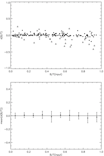
Fig. 1 shows the difference dðB/TÞ ¼ B/TðmeasuredÞ 2 B/TðinputÞ as a function of the input magnitude. For galaxies brighter than I ¼ 23 mag, dðB/TÞ is less than 0.1. This is a very accurate determination of this parameter. Fig. 2 shows dðB/TÞ as a function of B/TðinputÞ. Objects with I $ 23 (triangles) have bigger dispersion of dðB/TÞ than objects with I # 23 (full circles). From our simulations it follows that I ¼ 23 mag is the limiting magnitude for reliable recovery of the B/T parameter. The limiting magnitude for the rest of the structural parameters will be studied in a forthcoming paper. To our limiting apparent magnitude, the sample of galaxies is reduced to 120 galaxies. According to their B/T ratio, absolute magnitude and visual inspection (see Section 3), they were classified as: ellipticals (26), dwarfs (6), S0 (9), irregulars (20), mergers (17) and spirals (42). This left us with , 34 per cent spheroidal galaxies (E þ dwarfs þ S0), , 35 per cent

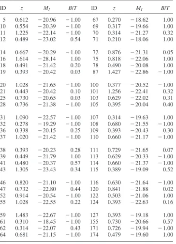
spirals, and , 31 per cent unclassified objects. Tables 1 and 2 show the B/T ratios (column 4) and MI(column 3) for the 120 galaxies

with I # 23:0 for the SSA13 and SSA22, respectively. These tables also show the identification number (column 1) and the redshift of the objects (column 2) given by Cowie et al. (1996). Galaxies classified as ellipticals and dwarfs have B/T ¼ 1:0, and those classified as irregular or mergers have B/T ¼ 21:0.

4.2 Completeness as function of redshift

In order to be sure that we are studying the same kind of object at different redshifts, we must determine the absolute limiting magnitude of our sample. On doing this we avoid biasing our sample to brighter objects at high redshift. Some claims of galactic evolution have been a consequence of this bias. As an example, Simard et al. (1999) analysed the problem of the completeness of the sample. If selection effects were ignored in their galaxies, then the mean disc surface brightness increases by < 1.3 mag from z ¼ 0:1 to z ¼ 0:9. Most of this evolution is plausibly due to comparing low-luminosity galaxies in nearby redshift bins to high-luminosity galaxies in distant bins. If this effect is taken into account, no discernible evolution remains in the disc surface brightness of their disc-dominated galaxies. In order to avoid this

Figure 1.(Top) The difference dðB/TÞ ¼ B/TðmeasuredÞ 2 B/TðinputÞ as a function of the input magnitude. (Bottom) Mean dðB/TÞ versus input magnitude with 1serror bars.

Figure 2. (Top) The difference dðB/TÞ ¼ B/TðmeasuredÞ 2 B/TðinputÞ versus B/TðinputÞ for two different magnitude intervals: I # 23 (full circles) and I . 23 (triangles). (Bottom) Mean dðB/TÞ versus B/TðinputÞ with 1serror bars.

kind of problem, it is necessary to make a selection of the objects on the basis of their absolute luminosity.

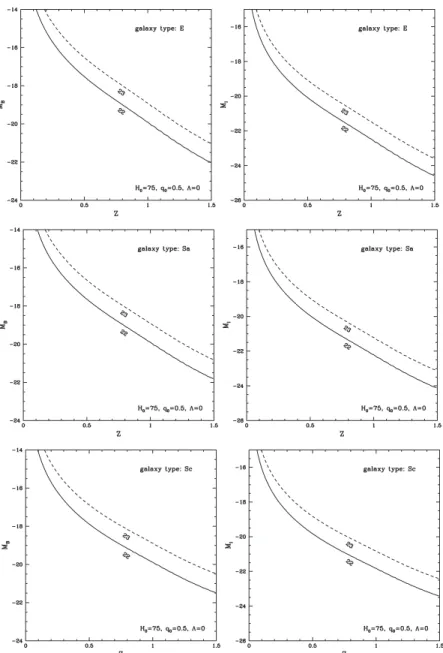
Given our apparent limiting magnitude of I ¼ 23, we have studied the completeness of our sample for three different classes of galaxies: Sa, Sc and E. Fig. 3 shows, for a limiting magnitude of I ¼ 23, the absolute magnitude down to which a galaxy can be observed as a function of z. This figure was generated using spectral models of 15 Gyr old galaxies (Poggianti 1997). For our distribution of 120 objects with I # 23, the parameters that maximize the number of objects into a complete sample are z # 0:8 and MI# 220:0 ðMB# 218Þ.4This left us with a total of 61

objects: 20 E/S0, 25 spirals, and 16 irregulars and mergers, or equivalently , 33 per cent E/S0, , 41 per cent spirals, and , 26 per cent unclassified objects. Fig. 4 shows the M versus z diagram for our whole sample down to I # 23. The complete subsample studied (bottom left rectangle) is enclosed by horizontal and vertical lines. This kind of selection criterion is similar to that used by Simard et al. (1999) and Fried et al. (2001).

5 R E S U LT S A N D D I S C U S S I O N 5.1 Galaxy classification

There is no substantial difference between the fractions of galaxies that correspond to the different classes when the sample is restricted in apparent or absolute magnitude. We must note that

these numbers are in good agreement with the percentage of E/S0 given by visual classification systems (van den Bergh et al. 1996, 2000) in the HDF, but are quite different from that (8 per cent) given by the automated classification of Marleau & Simard (1998). The classification of Marleau & Simard (1998) takes into account all objects with I814# 26 from the HDF. They claim that the

discrepancy with visual classifications is due to the difference in the classification of small round galaxies with half-light radii less than 00:31. Visually these galaxies are classified as elliptical galaxies, Marleau & Simard classify them as disc-dominated systems with bulge fractions less than 0.5. However, galaxies with an intrinsically large B/T tend to be systematically obtained with lower values of B/T in their automated routine (see fig. 10 of Marleau & Simard 1998). The ellipticals in the HDF that have (probably) been mis-classified by these authors are those principally coming from the fainter subsample. Although no relation between the B/T output of their simulation and the input magnitude of the objects is provided by these authors (and consequently our assertions must be taken with caution), it is certainly possible that the B/T results are more strongly affected on increasing the input magnitude (i.e. at lower signal ratios), and for that reason the high-redshift population of elliptical galaxies remains biased. By using an automated procedure which avoids this problem, we have been able to obtain a result similar to van den Bergh et al. (1996, 2000).

Table 1.Galaxies from SSA13 with I # 23:0.

ID z MI B/T ID z MI B/T 5 0.612 2 20.96 2 1.00 67 0.270 2 18.62 1.00 10 0.554 2 20.39 2 1.00 69 0.317 2 19.66 1.00 11 1.225 2 22.14 2 1.00 70 0.314 2 21.27 0.32 12 0.489 2 23.02 0.54 71 0.210 2 18.06 1.00 14 0.667 2 20.29 2 1.00 72 0.876 2 21.31 0.05 16 1.614 2 28.14 1.00 75 0.818 2 22.06 1.00 18 0.491 2 21.42 0.20 78 0.490 2 20.08 1.00 19 0.393 2 20.42 0.03 87 1.427 2 22.86 2 1.00 20 1.028 2 21.65 2 1.00 100 0.377 2 20.52 2 1.00 21 0.443 2 20.42 0.10 101 1.256 2 22.41 0.32 25 0.730 2 20.65 0.03 103 0.629 2 22.02 0.31 28 0.736 2 21.38 2 1.00 105 0.395 2 20.04 0.40 31 1.090 2 22.57 2 1.00 107 0.314 2 19.63 1.00 32 0.278 2 19.29 2 1.00 108 0.680 2 21.55 2 1.00 36 0.338 2 20.15 0.25 109 0.393 2 20.43 0.30 37 1.020 2 21.42 2 1.00 110 0.660 2 21.17 2 1.00 38 0.393 2 20.23 0.28 111 0.729 2 21.65 0.07 39 0.449 2 21.79 1.00 113 0.629 2 20.33 2 1.00 41 0.480 2 20.37 0.57 114 0.660 2 21.37 2 1.00 43 1.305 2 23.43 0.34 115 0.389 2 19.09 0.52 46 0.820 2 21.10 2 1.00 116 0.630 2 21.64 2 1.00 47 0.732 2 22.80 0.44 120 0.841 2 21.88 0.02 52 0.914 2 20.54 2 1.00 122 0.503 2 21.06 1.00 55 1.028 2 22.55 0.22 124 0.393 2 22.63 0.16 59 1.483 2 22.67 2 1.00 127 0.393 2 19.18 1.00 61 0.310 2 18.45 2 1.00 155 0.730 2 20.66 0.57 62 0.314 2 22.07 0.43 171 0.726 2 19.94 2 1.00 64 0.681 2 21.15 2 1.00 174 0.479 2 19.60 1.00

Table 2. Galaxies from SSA22 with I # 23:0.

ID z MI B/T ID z MI B/T 9 1.093 2 21.98 0.04 80 1.669 2 24.09 2 1.00 11 0.626 2 20.41 0.19 81 0.384 2 19.47 2 1.00 13 0.653 2 20.34 0.34 82 0.384 2 20.61 1.00 14 0.538 2 21.30 1.00 83 0.510 2 20.18 0.12 19 0.294 2 20.52 0.14 87 0.306 2 19.00 0.47 20 0.663 2 19.58 2 1.00 89 1.151 2 22.46 0.41 28 0.247 2 21.41 0.04 90 0.412 2 19.52 1.00 30 0.751 2 21.78 0.34 91 0.513 2 20.13 1.00 32 1.024 2 22.54 2 1.00 92 0.381 2 20.94 0.50 33 0.707 2 22.07 1.00 93 0.377 2 19.95 1.00 38 1.208 2 24.05 1.00 96 0.290 2 22.21 1.00 44 0.672 2 21.88 0.51 100 0.303 2 19.93 1.00 45 0.132 2 18.15 0.53 102 0.824 2 22.39 0.20 46 0.912 2 22.04 0.08 103 1.159 2 23.70 1.00 47 0.173 2 17.38 1.00 108 0.588 2 21.25 2 1.00 49 0.707 2 20.98 0.37 111 0.302 2 18.47 0.21 50 0.538 2 21.22 0.09 118 0.816 2 21.36 0.36 51 0.536 2 21.11 2 1.00 123 0.095 2 19.04 0.11 54 0.418 2 20.67 2 1.00 124 0.671 2 20.81 2 1.00 55 0.815 2 21.58 2 1.00 125 0.873 2 22.00 0.24 56 0.318 2 17.80 0.23 127 0.695 2 21.39 1.00 59 0.418 2 20.58 0.50 143 1.102 2 22.31 0.09 60 1.392 2 19.54 2 1.00 147 0.514 2 21.24 1.00 67 0.588 2 19.45 2 1.00 148 0.876 2 22.41 2 1.00 69 0.692 2 21.67 1.00 150 0.795 2 22.11 1.00 70 0.348 2 20.62 0.38 152 0.617 2 22.27 0.17 71 0.132 2 16.72 1.00 154 0.614 2 22.09 1.00 72 0.787 2 21.07 0.07 155 0.665 2 20.71 1.00 73 0.822 2 23.08 1.00 161 0.960 2 22.65 1.00 75 0.724 2 20.13 2 1.00 166 0.378 2 18.76 1.00 77 1.020 2 22.11 0.36 172 0.378 2 19.93 2 1.00 78 0.823 2 21.49 0.55 204 0.709 2 19.77 2 1.00 4

We have repeated this calculation with the starburst galaxy NGC 4449 without finding any substantial difference.

Interestingly, our sample and the HDF one are imaging a galaxy population centred around z , 0:5, the principal difference being in the exposure time. Because of the different depth in the images, substantial differences would be expected for the fainter subpopulation (smaller and irregular galaxies) between our sample and those based on the HDF. In fact, the HDF apparent magnitude-limited sample contains 39 per cent of unclassified objects whereas we obtain , 30 per cent.

5.2 Galaxy evolution

The two main models of galaxy evolution (monolithic collapse and hierarchical clustering) present a completely different scenario of galaxy evolution, so that the observational implications are also very different. One of these concerns the comoving density of the galaxies. In the redshift interval studied, the hierarchical model framework proposes that the comoving density of big galaxies (E/S0s and spirals) decreases with redshift, being constant in the

Figure 3.The complete magnitude as a function of the redshift for objects with apparent magnitudes: I ¼ 22 (full line) and I ¼ 23 (dashed line). Three different kinds of object are represented: ellipticals (top), Sa (middle) and Sc (bottom). See text for details.

Figure 4.The MIversus z diagram for the galaxies detected in the SSA13

and SSA22 fields. The absolute magnitudes have been computed for a H0¼ 75 km s21Mpc21, Vm¼ 1 and q0¼ 0:5 cosmology.

monolithic model. We have computed the comoving density r(z) for these two different types of galaxy in our complete subsample. To model the comoving density, we have assumed both a linear function of the form

rðzÞ ¼ a þ bz; ð3Þ

and a power law of the form

rðzÞ ¼ að1 þ zÞb; ð4Þ

where a ¼ rð0Þ is the comoving density at z ¼ 0 and b ¼ ½rðzmaxÞ 2 rð0ފ/zmax; with zmaxthe maximum value that z reaches

in our limiting subsample.

To reduce the loss of information in our data, we avoid binning them. The values of the parameters of the function r(z) are achieved by running a Kolmogorov – Smirnov test between the cumulative probability distribution function of finding a galaxy inside our imaging solid angle at a particular z given r(z) and the cumulative distribution from the real data. The cumulative probability function for our model is computed as

PðzÞ ¼ ðz zmin rðz0Þr2_ðz0_{Þðdr/dzÞ dz}0 ðzmax zmin rðz0Þr2_ðz0_{Þðdr/dzÞ dz}0; ð5Þ

where zminis the closest galaxy redshift, zmax¼ 0:8 for our limiting

subsample and r(z) is the comoving distance to an object placed at z.

The Kolmogorov– Smirnov (KS) test gives the probability that two data sets come from the same distribution. The best comoving density is that which maximizes this probability.

As a matter of caution, we must note that E/S0 galaxies are placed preferentially in high-density environments, being more strongly clustered than other types of galaxy. In order to evaluate the effect of clustering in our comoving density, we have studied the contribution of the E/S0 galaxies of each field to our cumulative function. The number of galaxies in the regions of more accumulation ð0:48–0:54 and 0:69–0:73Þ come from both fields with approximately the same contribution, rejecting a clustering explanation.

To evaluate the errors on the parameters in the E/S0 and in the spiral sample, we have assumed that a least two galaxies in each sample are mis-classified. This represents , 10 per cent of each sample. We construct all the subsamples that can be obtained by removing two elements from the original samples and then we recover the values of the parameters associated with them. Using these values we estimate the median and the standard deviation. These are the numbers that we present as the parameter estimations and the errors associated with these measurements. Fig. 5 shows the original whole sample (i.e. without removing any point) and overplotted is the cumulative function associated with the parameters measured as explained before. Error bars in Fig. 5 were estimated by measuring at each point the maximum distance between the cumulative function represented by using the whole sample and all the cumulative functions resulting from the previous subsamples. We have also overplotted the cumulative distribution obtained from the comoving densities fitted by Fried et al. (2001), who have a similar absolute magnitude cut for their sample ðMB# 218:5Þ.

The comoving density of the E/S0s that gives a maximum

probability in the KS test for a linear form is given by rðzÞ ¼ 0:0033ð^0:0015Þ 2 0:0015ð^0:0010Þ £ z:

The KS probability of this density is 0.90. This comoving density is closer to that deduced by Fried et al. (2001). Using their fit to our sample we obtain a KS p (KS pF) of 0.87. The number of E/S0s

decreases with redshift. For the cosmology chosen, this decrease is , 45(^ 30) per cent. On using the power-law model, the KS probability is slightly better, 0.92; we have

rðzÞ ¼ 0:0039ð^0:0018Þ £ ð1 þ zÞ21:6ð^0:4Þ:

In this case, the decrease of elliptical galaxies is , 60(^ 10) per cent. This behaviour is in a very good agreement with the prediction from the hierarchical clustering scenario for this cosmology (Baugh, Cole & Frenk 1996; Kauffmann, Charlot & White 1996) but differs from the results presented in Totani & Yoshii (1998) and Im et al. (2002). Interestingly, Daddi (2001) has pointed out that strong discrepancies in the number density evolution for the EROs (extremely red objects5) can be understood

Figure 5.The cumulative number distribution function of E/S0s (top) and spirals (bottom) as a function of the redshift. The best fits derived from linear and quadratic comoving densities are overplotted. Also shown are the cumu-lative distributions derived from Fried et al. (2001). See text for more details.

5

in terms of cosmic variance: ‘it is much probable, on average, to underestimate the true ERO surface density with small area surveys’. Maybe a similar explanation also holds for a more modest redshift E/S0 population, and this can be of help to understand the discrepancies in the number density evolution pointed out by different authors.

For the spirals, the comoving density is rðzÞ ¼ 0:0069ð^0:0025Þ þ 0:0014ð^0:0006Þ £ z;

but the KS probability is just 0.78. The parameters of the power-law model for this family are rð0Þ ¼ 0:0060ð^0:0031Þ and m ¼ 1:7ð^0:5Þ with a KS probability of 0.92. Interestingly, for this population a peak in the range z ¼ 0:4–0:5 is shown in the comoving density obtained from binned data in Fried et al. (2001), although they fit only a linear comoving density. Probing on this possibility, we have also tested a quadratic comoving density,

rðzÞ ¼ a þ bz þ cz2 ð6Þ

where the interpretation of these parameters is as follows: a ¼rð0Þ, b ¼ 2Dr/zp [where zp is the redshift at which the

comoving density reaches its highest value and Dr ¼ rðzpÞ 2 rð0ފ

and c ¼ 2Dr/z2

p. Using a quadratic comoving density we obtain

the highest probability, 0.96, with the next values for the parameters:

rðzÞ ¼0:0095ð^0:0036Þ þ 0:0027ð^0:0012Þ £ z 2 0:0031ð^0:0018Þ £ z2_:

Notice that this implies a peak of the density at z ¼ 0:43. Nevertheless, the value of the comoving density at this peak is just 6 per cent higher that at z ¼ 0. Meanwhile the value of the density at z ¼ 0:8 is slightly higher (about 1 per cent) than at z ¼ 0. Consequently, contrary to the E/S0s, brighter spiral galaxies ðMB# 218Þ seem to have a relatively quiet evolution.

Our values of r(0) for E/S0 and spiral galaxies are in good agreement with the values that can be obtained by using the fit to the Schechter luminosity function (Schechter 1976) of nearby samples (Marzke et al. 1998). For MB# 218, the local comoving

density is rð0Þ ¼ 0:0026 ^ 0:0007 (E/S0s) and rð0Þ ¼ 0:0054 ^ 0:0014 (spiral galaxies).

We have also evaluated the previous quantities assuming a different cosmology: Vm¼ 0:3 and VL¼ 0:7. In this case, our

absolute magnitude limit is MB# 219. We summarize our results

in Table 3. The E/S0 comoving density at this cosmology seems not to evolve or to decrease slightly. This is a similar result to that obtained for this cosmology by Totani & Yoshii (1998) and Im et al. (2002) and what is expected from semi-analytical hierarchical models (e.g. Kauffmann & Charlot 1998). The results for the spiral galaxies are compatible with no number density evolution.

6 C O N C L U S I O N S

We present the quantitative morphology of galaxies in two Hawaiian Deep Fields imaged by six HST fields. Down to the limiting magnitude of our sample, nearly all galaxies have spectroscopic redshifts. The morphology has been obtained by fitting a pure Se´rsic and Se´rsic plus exponential profiles to the surface brightness distribution of the galaxies. Monte Carlo simulations have been carried out in order to determine the limiting magnitude down to which the recovered structural parameters are reliable. The galaxies have been classified according to the B/T ratio. E/S0 systems are those with B/T . 0:5. Our simulations suggest an apparent magnitude limit of I ¼ 23. We have also accurately determined the absolute limiting magnitude of our sample MB# 218. The complete subsample is composed of 61

objects up to z ¼ 0:8.

The percentages of the different galaxy types in the whole sample are in good agreement with those obtained in the HDF by visual methods. We have computed the comoving density of the galaxies as a function of redshift. For an Einstein – de Sitter universe, the comoving density of E/S0s decreases as z increases, in very good agreement with the predictions of hierarchical clustering models of galaxy evolution. The comoving density of spiral galaxies shows a good fit to a quadratic form: it grows , 6 per cent from z ¼ 0 until z ¼ 0:43, and then decreases slightly until z ¼ 0:8. This fit is compatible with no number evolution. For open or L universes, the E/S0 galaxies comoving density is compatible with no number density evolution or a slight decrease as expected from semi-analytical models in hierarchical clustering scenarios. Comoving density for brighter spiral galaxies also remains quite constant at this redshift range.

A C K N O W L E D G M E N T S

We wish to thank David Cristo´bal and Juan Betancort for valuable discussions. We are also indebted to Victor Debattista who kindly

Table 3.Parameters of the comoving density; H0¼ 75 km s21Mpc21.

Model Type a b c KS p KS pF Vm¼ 1, VL¼ 0 a þ bz E/S0 0.0033(^ 0.0015) 2 0.0015(^ 0.0010) – 0.90 0.87 að1 þ zÞb _{E/S0 0.0039(^ 0.0018) 2 1.6(^ 0.4) – 0.92 –} a þ bz S 0.0069(^ 0.0025) 0.0014(^ 0.0006) – 0.78 0.70 að1 þ zÞb S 0.0060(^ 0.0031) 1.7(^ 0.5) – 0.92 – a þ bz þ cz2 _{S 0.0095(^ 0.0036) 0.0027(^ 0.0012) 2 0.0031(^ 0.0018) 0.96 –} Vm¼ 0:3, VL¼ 0:7 a þ bz E/S0 0.0049(^ 0.0026) 0.0032(^ 0.0040) – 0.86 0.83 að1 þ zÞb _{E/S0 0.0055(^ 0.0024) 2 1.1(^ 0.3) – 0.82 –} a þ bz S 0.0071(^ 0.0022) 2 0.0019(^ 0.0027) – 0.81 0.73 að1 þ zÞb _{S 0.0043(^ 0.0025) 1.5(^ 0.4) – 0.85 –} a þ bz þ cz2 _{S 0.0063(^ 0.0042) 0.0017(^ 0.0011) 2 0.0012(^ 0.0015) 0.87 –}

proofread versions of this manuscript. The authors are grateful to the anonymous referee for valuable suggestions that helped us to improve the rigour and clarity of this paper.

The work reported herein is based on observations with the NASA/ESA Hubble Space Telescope obtained at the Space Telescope Science Institute, which is operated by the Association of Universities for Research in Astronomy, Inc., under NASA contract 5-26555.

R E F E R E N C E S

Abraham R. G., Tanvir N. R., Santiago B. X., Ellis R. S., Glazebrook K., van den Bergh S., 1996, MNRAS, 279, L47

Baugh C., Cole S., Frenk C., 1996, MNRAS, 283, 1361 Bertin E., Arnout S., 1996, A&AS, 117, 393

Brinchmann J. et al., 1998, ApJ, 499, 112

Caon N., Capaccioli M., D’Onofrio M., 1993, MNRAS, 265, 1013 Conselice C. J., Bershady M. A., Jangren A., 2000, ApJ, 529, 886 Cowie L. L., Gardner J. P., Hu E. M., Songaila A., Hodapp K. W.,

Wainscoat R. J., 1994, ApJ, 434, 114

Cowie L. L., Hu E. M., Songaila A., 1995, AJ, 110, 1576 Cowie L. L., Songaila A., Hu E. M., 1996, AJ, 112, 839 Daddi E., 2001, Ap&SS, 277, 531

Eggen O. J., Lynden-Bell D., Sandage A., 1962, ApJ, 136, 748 Frei Z., Guhathakurta P., Gunn J. E., Tyson J. A., 1996, AJ, 111, 174 Fried J. W. et al., 2001, A&A, 367, 788

Im M. et al., 2002, ApJ, in press Kauffmann G., 1996, MNRAS, 281, 478

Kauffmann G., Charlot S., 1998, MNRAS, 294, 705

Kauffmann G., White S., Guiderdoni B., 1993, MNRAS, 264, 201 Kauffmann G., Charlot S., White S. D. M., 1996, MNRAS, 283, L117

Larson R. B., 1975, MNRAS, 166, 585 Le Fevre O. et al., 1999, MNRAS, 311, 565 Marleau F. R., Simard L., 1998, ApJ, 507, 585

Marzke R., da Costa L. N., Pellegrini P. S., Willmer C. N. A., Geller M. J., 1998, ApJ, 503, 617

Poggianti B. M., 1997, A&AS, 122, 399

Press W. H., Teukolsky S. A., Vetterling W. T., Flannery B. P., 1992, Numerical Recipes. Cambridge Univ. Press, Cambridge

Prieto M., Aguerri J. A. L., Varela A. M., Munoz-Tuno´n C., 2001, A&A, 267, 405

Schade D., Lilly S., Le Fevre O., Hammer F., Crampton D., 1996, ApJ, 464, 79

Schade D. et al., 1999, ApJ, 525, 31 Schechter P., 1976, ApJ, 203, 297

Se´rsic J., 1968, Atlas de Galaxias Australes. Obs. Astrono´mico, Co´rdoba Simard L. et al., 1999, ApJ, 519, 563

Simien F., de Vaucouleurs G., 1986, ApJ, 302, 564

Songaila A., Cowie L. L., Hu E. M., Gardner J. P., 1994, ApJS, 94, 46 Totani T., Yoshii Y., 1998, ApJ, 501, L177

Trujillo I., Aguerri J. A. L., Cepa J., Gutie´rrez C. M., 2001a, MNRAS, 321, 269

Trujillo I., Aguerri J. A. L., Gutie´rrez C. M., Cepa J., 2001b, AJ, 122, 38 Trujillo I., Aguerri J. A. L., Gutie´rrez C. M., Cepa J., 2001c, MNRAS, 328,

977

van den Bergh S., Abraham R. G., Ellip R. S., Tanvir N. R., Santiago B. X., Glazebrook K., 1996, AJ, 112, 359

van den Bergh S., Cohen J. G., Hogg D. W., Blandford R., 2000, AJ, 120, 2190

White S., Rees M., 1978, MNRAS, 183, 341