It is Not Just Confusion! Strategic Uncertainty in an Experimental Asset Market

(1)

HAL Id: halshs-01294917

https://halshs.archives-ouvertes.fr/halshs-01294917

Submitted on 7 Sep 2016

HAL is a multi-disciplinary open access

archive for the deposit and dissemination of

sci-entific research documents, whether they are

pub-lished or not. The documents may come from

teaching and research institutions in France or

L’archive ouverte pluridisciplinaire HAL, est

destinée au dépôt et à la diffusion de documents

scientifiques de niveau recherche, publiés ou non,

émanant des établissements d’enseignement et de

recherche français ou étrangers, des laboratoires

It is Not Just Confusion! Strategic Uncertainty in an

Experimental Asset Market

Eizo Akiyama, Nobuyuki Hanaki, Ryuichiro Ishikawa

To cite this version:

Eizo Akiyama, Nobuyuki Hanaki, Ryuichiro Ishikawa. It is Not Just Confusion! Strategic

Un-certainty in an Experimental Asset Market. Economic Journal, Wiley, 2017, 127, pp.F563-F580.

�10.1111/ecoj.12338�. �halshs-01294917�

(2)

It is not just confusion!

Strategic uncertainty in an experimental asset market

∗

Eizo Akiyama

Nobuyuki Hanaki

Ryuichiro Ishikawa

Abstract

To what extent is the observed mispricing in experimental asset markets caused by strategic uncertainty and by confusion? We address this question by comparing subjects’ initial price forecasts in two market environments: one with six human traders, and the other with one human and five computer traders. We find that both strategic uncertainty and confusion contribute equally to the median initial forecast deviation from the fundamental value. The eﬀect of strategic uncertainty is greater for subjects with a perfect score in the Cognitive Reflection Test, and it is not significant for those with low scores.

To what extent are the observed price deviations from the fundamental value in exper-imental asset markets (Smith et al., 1988) caused by strategic uncertainty (uncertainty about the behaviour of others) and by individual bounded rationality (or confusion)? First, we describe the context in which this question is posed.

Consider an asset with a finite life of T periods. Each unit of the asset pays a constant dividend D at the end of each period, and becomes worthless after the final dividend payment at the end of period T . Under these conditions, the fundamental value of a unit of the asset during period t (t = 1, 2, ..., T ), F Vt, is the sum of the remaining dividend

payments, i.e., F Vt= (T + 1− t)D. If these conditions are commonly known, common

knowledge of rationality implies that if rational traders trade this asset, it will only be at its fundamental value.

Following the seminal study by Smith et al. (1988), it has repeatedly been shown for a variety of experimental conditions and subject pools, that the market prices of assets

∗_{Corresponding author: Nobuyuki Hanaki. GREQAM, Aix-Marseille Universit´}_{e, 3 Ave. Robert}

Schuman, 13628 Aix-en-Provence, Cedex 1, France. E-mail: nobuyuki.HANAKI@univ-amu.fr. Hirofumi Kimiatsuku, Michiko Ogaku, Makoto Soga, and Hiroto Yonenoh provided invaluable help in organising the experiments. This project is partly financed by a Japan Society for the Promotion of Science (JSPS) Centre National de la Recherche Scientifique (CNRS) bilateral research grant, a JSPS -Agence Nationale de la Recherche (ANR) bilateral research grant “BECOA” (ANR-11-FRJA-0002), and financial aid from the Japan Center for Economic Research and Japan Securities Scholarship Foundation. The experiments reported in this paper were approved by the Institutional Review Board of the Faculty of Engineering, Information and Systems, University of Tsukuba (No. 2012R25).

(3)

deviate substantially from their fundamental value in these experimental asset markets.1

Such deviations in observed prices from the fundamental value (mispricings) were initially considered to result from strategic uncertainty (i.e., uncertainty about others’ behaviour) by Smith et al. (1988). They noted that ‘what we learn from the particular experiments reported here is that a common dividend, and common knowledge thereof, is insuﬃcient to induce initial common expectations. As we interpret it, this is due to agent uncertainty about the behaviour of others’ (Smith et al., 1988, p.1148).

An implication of this is what Lei et al. (2001) called a “speculative hypothesis.” That is, ‘traders are uncertain that future prices will track the fundamental value, because they doubt the rationality of the other traders, and therefore speculate in the belief that there are opportunities for future capital gains’ (Lei et al., 2001, p.832). Lei et al. (2001) tested the “speculative hypothesis” by performing a set of experiments in which capital gains were not possible because resale of the assets was prohibited. Based on the observed mispricings even in the absence of capital gain possibilities, Lei et al. (2001) rejected the speculative hypothesis and noted that ‘the hypothesis that the traders are rational, and that the bubble is due to the fact that this rationality is not common knowledge, cannot be the whole story behind the bubbles’ (p.857). Instead, they suggested the “active participation hypothesis”; i.e., subjects in these experiments who were trained to engage in trading simply wanted to trade (even if such trading resulted in incurring losses) because there were no other activities available to them during the experiment.

Huber and Kirchler (2012) and Kirchler et al. (2012) also suggested that these mis-pricings were mainly due to subjects being confused about the nature of the declining fundamental value of the asset in the experiment. Kirchler et al. (2012) also showed that mispricing due to confusion was further fuelled by increasing the amount of cash relative to the number of assets available in the market as a result of dividend payments during the experiment.2

1_{In the original experiment in Smith et al. (1988) as well as in many other studies, the value of the}

dividend payment in each period, dt, was determined randomly from a known i.i.d. distribution. Thus,

the fundamental value of the asset was defined as F Vt = ∑Tp=tE(dt), where E(dt) is the expected

dividend payment. Porter and Smith (1995) eliminated the uncertainty about dividend payments by investigating the eﬀect of varying degrees of risk aversion among subjects. No significant diﬀerence was found in the observed pattern of mispricing in the experiments with uncertain dividend payments. See St¨ockl et al. (2010) and Palan (2013) for surveys.

2_{This conclusion is in contrast with an earlier study by Noussair et al. (2001) that showed substantial}

(4)

These studies showed that the magnitude of mispricing became much smaller if in the instructions, an illustration of the declining fundamental value was presented to the subjects, rather than a table containing the same information (Huber and Kirchler, 2012), or if the word “stock” (the value of which many subjects assumed did not decline constantly) was explained as “stocks of a depletable gold mine” (Kirchler et al., 2012).

Is it just confusion (i.e., subjects not understanding the declining fundamental value in these experiments that is not natural in real markets) causing the mispricing? It would be quite surprising, however, if all the subjects in the experiments were equally confused given the widely reported heterogeneity in the depth of strategic thinking among subjects in laboratory experiments (Nagel, 1995; Ho et al., 1998; Costa-Gomes and Crawford, 2006).3 In addition, several studies demonstrated both theoretically (Haltiwanger and Waldman, 1985, 1989) and experimentally (Fehr and Tyran, 2008; Sutan and Willinger, 2009; Heemeijer et al., 2009; Bao et al., 2012) that such heterogeneity could manifest as a large deviation from the equilibrium in the presence of positive feedback.4 _{Because it is}

very likely that positive feedback exists in asset markets, confusion or bounded rational behaviour of a few subjects in a market can be amplified owing to strategic responses by more sophisticated subjects. This consideration leads us to our main research question: to what extent is mispricing caused by confusion (or some kind of individual bounded rationality) and strategic uncertainty? The above-mentioned studies did not investigate these questions, and thus the relevance of strategic uncertainty in these experiments remains an open question.

In this paper, we address this open question by eliminating strategic uncertainty as much as possible by introducing computer traders who follow the equilibrium strategy (under the usual set of assumptions of profit maximisation and the common knowledge of rationality). We consider two types of markets (treatments) consisting of six traders: one human and five computers (1H5C), and six humans (6H). All subjects were informed of which treatment they were involved in, and those in 1H5C, but not those in 6H, were

3_{The theoretical developments that follow these experimental findings suggest that considering}

in-teraction among heterogeneous boundedly rational agents helps us to better understand experimental outcomes. See Camerer (2003, Ch.5) and Crawford et al. (2013) for further details.

4_{These experimental analyses considered diﬀerent games. Fehr and Tyran (2008) considered price}

setting games, Sutan and Willinger (2009) investigated beauty contest games, while both Heemeijer

et al. (2009) and Bao et al. (2012) investigated price forecasting games. What these studies also showed

was that in the presence of strategic substitution (or negative feedback), the observed outcomes were much closer to the Nash or rational expectation equilibrium.

(5)

clearly told how computer traders behave. Therefore, in the 1H5C treatment, the single

human trader did not face any strategic uncertainty. Here we mention a couple of

additional design aspects before discussing how our experimental design enabled us to achieve our objective.

To facilitate the introduction of computer traders, we employ a call market rule similar to those used by van Boening et al. (1993) and Haruvy et al. (2007) rather than the continuous double auction employed by Smith et al. (1988) and in various other studies. In a call market, traders submit buy (sell) orders by specifying the maximum (minimum) price they are willing to pay (accept) for a unit of asset in each period. This means that our computer traders, in each period, submit their buy orders (sell orders) by specifying the fundamental value of the asset in that period as the maximum (minimum) price they are willing to pay (accept) for a unit of asset. Once all the traders in the market have submitted their orders, the price that clears the market is calculated, and all transactions take place at that price among traders who submitted a maximum buying price no less than, or a minimum selling price no greater than, the market-clearing price. Note, however, that because of the way computer traders behave, the market prices in 1H5C follow the fundamental value very closely. Thus, comparing the realised market

prices for the two treatments, 6H and 1H5C, is not informative for our purposes.

In-stead, we elicit subjects’ expectations about future prices as in Haruvy et al. (2007), and compare them for the two treatments. It has been shown that expected future prices deviate quite substantially from the fundamental value in all human markets (Haruvy

et al., 2007, Figure 3, p. 1909), and that the deviations disappear gradually as subjects

gain experience from trading under the same market conditions. This is similar to what is observed from the realised prices. Thus, our focus on price forecasts is informative for studying the cause of realised price deviations.

How then does our design allow us to identify the eﬀect of strategic uncertainty as well as individual bounded rationality (or confusion) in asset market experiments? Let us imagine a rational human trader. In the 1H5C treatment, s/he does not face any un-certainty regarding the behaviour of the other traders in the market. Moreover, given the behaviour of the computer traders, s/he would expect prices to follow the fundamental value. Therefore, if we observe any deviation from this expectation in our data, it must

(6)

be due to some kind of individual bounded rationality (or confusion). On the contrary, in the 6H treatment, the rational human trader is unsure about the behaviour of the other traders in the market and can expect a variety of outcomes. Of course, we should not eliminate the possibility that subjects are confused or boundedly rational. Thus, the observed deviations of price forecasts from the fundamental value in the 6H treatment are due to both strategic uncertainty and individual bounded rationality. A comparison of the subjects’ price expectations in the 1H5C and 6H treatments, therefore, gives us a direct measure of the extent to which strategic uncertainty explains the deviation of price forecasts from the fundamental value.

Several experiments have introduced computer agents that follow equilibrium be-haviour in laboratory experiments to reduce strategic uncertainty. Cason and Friedman (1997), in their experiments on price formation in a simple market institution,5 intro-duced robot traders that followed a Bayesian-Nash equilibrium strategy to facilitate learning by human subjects.6 _{Fehr and Tyran (2001) introduced robots that utilised a}

Nash equilibrium strategy in their investigation of nominal (money) illusion to decom-pose the reasons for non-immediate adjustment against negative nominal shocks into (i) those arising from individual irrationality, and (ii) those due to a lack of common knowledge of rationality.7 _{They reported that both individual irrationality (or bounded}

rationality) and the lack of common knowledge of rationality (or strategic uncertainty) contributed equally to the failure of immediate adjustment to the new equilibrium after a negative nominal shock in the game.8

5_{Cason and Friedman (1997) did not consider markets for assets with a life of several periods as we}

do in this paper.

6_{It should be noted that when human subjects play against other human subjects who are also}

learning, the learning process can be very slow. In addition to robots that follow the Bayesian-Nash equilibrium strategy (BNE robots), Cason and Friedman (1997) also introduced “revealing robots” whose behaviour diﬀered from that of the BNE robots, to investigate whether convergence to equilibrium was due to human subjects mimicking the behaviour of the BNE robots or to their best response against the BNE robots. Their results suggested the latter.

7_{Fehr and Tyran (2001) considered price-setting games by varying two aspects of the game: (a)}

whether negative nominal shocks were present; and (b) whether a human subject played the game with other human subjects or with rational computer programs that assumed all players were rational. This two-by-two design allowed them to achieve the objective of the experiments. This was also discussed quite extensively in Fehr and Tyran (2005).

8_{In addition to rational robots that followed the equilibrium strategy, Costa-Gomes and Crawford}

(2006) introduced boundedly rational robots that followed Level-1,2,3 or Dominance 1,2 strategies in their experiments on a two-person guessing game to better analyse the responses of human subjects who were informed about the behavioural rules of the various opponents. In a diﬀerent strand of the literature, computer agents were introduced to investigate whether deviations of observed behaviour from the equilibrium prediction were due to bounded rationality (confusion) or kindness in games such as an alternative oﬀer bargaining game (Johnson et al., 2002) or public good games (Houser and Kurzban,

(7)

Our experimental results suggest that strategic uncertainty accounts for about 50% of the median initial forecast deviation from the fundamental value; the remaining 50% is due to bounded rationality. Thus, it is not only confusion that causes mispricing in an experimental asset market; strategic uncertainty also plays an important role. To further investigate the effect of heterogeneity among subjects, we categorised subjects based on their scores in the Cognitive Reflection Test (Frederick, 2005, CRT) and analysed the data separately based on the CRT scores. We found that the effect of strategic uncertainty was much larger (about 70% of the median initial forecast deviation from the fundamental value) for those with a perfect CRT score. For those with very low CRT scores, on the other hand, no significant effect of strategic uncertainty was observed.

In a recent independently conducted study, Cheung et al. (2014) investigated the eﬀect of uncertainty regarding how others understood the nature of the fundamental value on mispricing in experimental asset markets by (1) training subjects extensively on the nature of the fundamental value, and (2) manipulating the subjects’ knowledge about whether others in the same market had received the same training. They found that the magnitude of mispricing was substantially smaller when all subjects in a market were trained and knew that all those in the market were trained than the case where all subjects in a market were trained but were not aware of this. Moreover, in the latter case, the mispricing was as great as in the case without training. Based on these results, Cheung et al. (2014) concluded that individual confusion alone could not account for the observed mispricing, but that uncertainty about how well others understood the nature of the fundamental value could.

While the setup of Cheung et al. (2014) diﬀers from ours in various respects,9it would be an interesting future study to investigate how the eﬀect of strategic uncertainty we have identified via price forecasts (which accounts for about 50% of the median forecast deviation) can be amplified so that it accounts for most of the mispricing as reported by Cheung et al. (2014).

The rest of the paper is organised as follows. The experimental design is discussed

2002). These studies identified substantial impact of bounded rationality.

9_{Cheung et al. (2014) used a setup with continuous double auctions, larger and longer markets (ten}

traders and 15 periods in each market), and stochastic dividends. Furthermore, they did not elicit price forecasts as we do in this paper.

(8)

in detail in Section 1. Section 2 presents the results of our experiments, and Section 3 concludes the paper.

1 Experimental Design

We set up an experimental call asset market consisting of six traders, who were either human subjects or computer programs, and considered two treatments. In the first, referred to as the 6H treatment, all six traders were human subjects. In the other, referred to as the 1H5C treatment, only one of the six traders was human, and the other five traders were computer traders who submitted orders at the fundamental value. In each treatment, subjects were explicitly told about the composition of the six traders in the market in which they were participating. Moreover, in the 1H5C treatment, subjects were also informed about the behaviour of the computer traders. Our main focus was to compare the data for these two treatments to separate the eﬀects of strategic uncertainty and individual bounded rationality.

In each market, traders could trade an asset with a life of 10 periods. Initially, all traders were endowed with four units of asset and 520 experimental currency units (ECUs, which we called Marks). Subjects were also asked to submit their expectations regarding the future prices of a unit of the asset. We first describe the trading rule employed, and then proceed to explain how subjects’ expectations about future prices were elicited.

We used a call market rule similar to that in Haruvy et al. (2007). In each period, each trader could submit at most one buy order and one sell order.10 _{An order consisted}

of a pair of values: a price and a quantity. When submitting a buy order, a trader had to specify the maximum price, P D, at which s/he was willing to buy a unit of asset, and the maximum quantity, QD, s/he was willing to buy. In the same manner, when submitting a sell order, a trader had to specify the minimum price, P S, at which s/he was willing to sell a unit of asset, and the maximum quantity, QS, s/he was willing to sell. We attached three constraints: the admissible price range, a budget constraint, and

10_{Of course, a trader could choose not to submit any orders by specifying zero as the quantity to}

buy and sell. We imposed a 60-second, non-binding, time limit for submitting orders. On reaching the time limit, subjects were simply informed through a flashing message in the upper right corner of their screens, to submit their orders as soon as possible.

(9)

the relationship between P D and P S in the case that a subject submitted both buy

and sell orders. The admissible price range was set so that, when QD ≥ 1 (QS ≥ 1),

P D (P S) was an integer between 1 and 2000, i.e., P D(P S) ∈ {1, 2, ..., 2000}. The

budget constraint simply meant that neither borrowing cash nor short selling an asset

was allowed, so that (i) QD× P D ≤ cash holding at the beginning of the period, and

(ii) QS ≤ units of asset on hand at the beginning of the period. The final constraint

was such that when a trader submitted both buy and sell orders, i.e., QD ≥ 1 and

QS ≥ 1, the maximum buying price was not greater than the minimum selling price,

i.e., P S≥ P D. Once all the traders in the market had submitted their orders, the price clearing the market was calculated,11 _{and all transactions were processed at that price}

among traders who submitted a maximum buying price no less than, or a minimum selling price no greater than the market-clearing price.12

At the end of each period, for each unit of the asset, 12 ECUs was paid as a dividend. We selected a fixed dividend payment, instead of a stochastic dividend as commonly considered in the literature, to eliminate all uncertainty other than strategic uncertainty from the experiment. The dividend could be used to purchase the asset in subsequent periods. After the final dividend was paid at the end of period 10, the asset had no value. Because the asset had no intrinsic value other than this stream of dividend payments, the fundamental value of a unit of asset at the beginning of period t was F Vt= 12×(11−t).

We distributed a table showing the sum of the remaining dividends after the dividend for each period had been paid out, a value we called the “next value” in the experiment. Thus, subjects had a table showing F Vtfor t = 1, 2, ..., 10 and could refer to it any time

during the experiment. This table is given in online Appendix A.

After explanation of the setup of the call market, as well as the table of fundamental values, subjects in the 1H5C treatment, but not those in 6H, were told the following about the behaviour of computer traders: “In each period, each computer trader places buy and sell orders by setting both the maximum price it is willing to pay and the minimum price it is willing to accept to the next value at the beginning of the period.”

11_{When there were several such prices, the lowest was chosen as the market-clearing price. This was}

important to ensure the price did not increase in the absence of transactions at the market-clearing price.

12_{Any ties among the last accepted buy or sell orders were resolved randomly. It was possible that no}

(10)

Thus, subjects were informed about the exact trading strategy employed by the computer traders.

Next, we explain how expectations about future prices were elicited. We basically fol-lowed the design used by Haruvy et al. (2007). At the beginning of each period, subjects were asked to submit their price forecasts for all the remaining periods in the market.13

In other words, in period t, each subject submitted 11−t forecasts.14 _{Therefore, subjects}

submitted a total of 55 price forecasts over the 10 periods. Subjects were informed that they would receive the following bonus payment based on how accurate their forecast prices were:

Bonus (in ECUs) = 0.5%

×(number of forecasts that were within ± 10% of the actual market price)

× final cash holding in period 10. (1)

Therefore, if all 55 forecasts were within 10% of the realised prices, the subject would receive 27.5% of his/her final cash holding as a bonus payment. This incentive scheme for accurate forecasts was chosen to reduce subjects’ incentive to influence the prices to move closer to their forecasts by incurring losses.15 _{During the submission of price}

forecasts, all previous market-clearing prices were shown on the screen.

The call market rule had several advantages: (i) the prices subjects had to forecast were clear; (2) learning based on observing orders submitted by other traders within a period was not possible; and (3) it was easier to introduce computer traders because all orders were submitted simultaneously.

At the end of each period, subjects were informed about the market-clearing price

13_{Although this was not stated explicitly in the instructions, each price forecast took the form of an}

integer value between 0 and 2000. We set this range to match the admissible values of orders. If subjects tried to submit a value outside this range, an error message stating that the forecast had to be within the given range was displayed on their computer terminal.

14_{We imposed a 120-second, non-binding time limit for submitting price forecasts. When the time}

limit was reached, subjects were simply told, through a message flashing in the upper right corner of their screens, to submit their forecasts as soon as possible.

15_{As noted by Haruvy et al. (2007), there is a trade-oﬀ between an incentive for accurate transactions}

and an incentive for maximising profit from trading. In other words, because we asked subjects to submit their forecasts before submitting their order, it could be possible that if the incentive for accurate forecasts was too great, subjects would submit potentially loss-making orders to influence the prices to move closer to their forecasts. In our design, since the bonus for accurate forecasts was a fraction of the final cash holding, this incentive was reduced. It is, of course, best to have both accurate forecasts and high profit from trading.

(11)

for the period, the units of asset they had traded,16 _{their cash and asset holdings, the}

number of price forecasts that were within 10% of the actual market prices up to that period, and the “next value” of a unit of the asset, which was equal to 12× (10 − t) at the end of period t.

The same group of traders, with identical initial endowments of cash and assets, repeated the same period market three times as one experiment. We refer to a 10-period market as a round.17

At the end of the experiment (after participating in three rounds of the 10-period market), subjects were paid in cash the sum of their final cash holdings (including the bonus payment for accurately predicting future market prices) for each round plus a participation fee of 500 yen. We used an exchange rate between ECUs and Japanese yen of 1 ECU = 1 Japanese yen. The experiment lasted about two and a half hours including the explanation of the instructions and completion of a questionnaire after the experiment.18 _{The questionnaire included the Cognitive Reflection Test (Frederick,}

2005). Subjects earned on average about 4000 yen.

2 Results

A series of computerised experiments were conducted at the University of Tsukuba be-tween May and July 2013. The experiments were implemented using z-tree (Fischbacher, 2007). A total of 173 subjects (72 subjects in 6H and 101 subjects in 1H5C), who had never participated in a similar experiment, were recruited from across the campus via e-mails and flyers. Subjects had to register on our database before the experiment, so that we could verify their lack of participation in past experiments by checking their names, student ID numbers, and e-mail addresses.

In this paper, we focus on the initial deviation of price expectations from the funda-mental value, realised prices, and dynamics on forecast deviations.

16_{In the presentation of this information, a positive (resp. negative) number denoted that they had}

bought (resp. sold) a certain number of units of asset.

17_{Before entering round 1, there was a practice period to allow subjects to familiarise themselves with}

the user interface of the software. Subjects were given their initial endowment of cash and assets, and asked to enter their price forecasts for the 10 periods and their orders for period 1. Information regarding the resulting market-clearing price, amongst others, was not shown to the subjects.

(12)

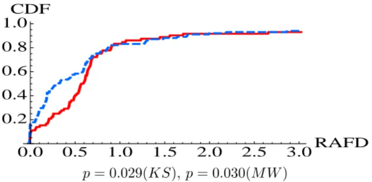
0.0 0.5 1.0 1.5 2.0 2.5 3.0RAFD 0.2 0.4 0.6 0.8 1.0 CDF p = 0.029(KS), p = 0.030(M W )

Fig. 1: Distributions of RAF D1,1 for 1H5C (dashed, N=101) and 6H (solid, N=72).

Note: In all subsequent figures, p-values are given for a Kolmogorov-Smirnov (KS) two-tailed test as well as a Mann-Whitney (MW) two-two-tailed test.

2.1 Deviation of Forecasts

In each period, subjects forecast prices for all the remaining periods within the round. To better summarise the magnitude of forecast deviations from the fundamental value (referred to as forecast deviations below) for each subject, we introduced a measure of forecast deviations similar to the mispricing metric, that is, the relative absolute deviation (RAD) proposed by St¨ockl et al. (2010).

For subject i, the magnitude of the forecast deviations for the forecasts submitted in period t of round r was measured by the relative absolute forecast deviation (RAF Dit,r)

defined as: RAFDi_t,r= 1 T− t + 1 T ∑ p=t |fi t,p,r− F Vp| F V (2)

where T is the number of periods (T = 10 in our experiments), fi

t,p,r is the forecast

of period p’s asset price submitted by subject i in period t of round r, F Vp is the

fundamental value of the asset in period p, and F V is the average fundamental value of the asset over all periods.19

Figure 1 shows the distributions of RAF Di

1,1 for 6H (solid lines) and 1H5C (dashed

lines). As shown in the figure, the observed distributions as well as the median values of

RAF Di

1,1 for the two treatments diﬀer significantly.

19_{We omit subscript r for F V}

p, F V , and T because these values remained constant over all three rounds

of our experiment. One could also consider normalising the measure using the average fundamental value of the asset over the remaining periods after period t. We avoided doing this to keep the denominator constant for all t.

(13)

Recall that the effect of individual bounded rationality (or confusion) is measured by the forecast deviations in the 1H5C treatments, while the effect of strategic uncertainty is measured by the difference between the forecast deviations for the 1H5C and 6H

treat-ments. Since the median RAF D1,1 values are 0.583 for 6H and 0.315 for 1H5C, about

54% (=0.315/0.583) of the median initial forecast deviation is due to individual bounded rationality, while the remaining 46% (0.268/0.583) is due to strategic uncertainty.

2.2 Cognitive Ability and Strategic Uncertainty

We identified a significant eﬀect of strategic uncertainty based on the price forecasts submitted at the beginning of round 1 in each experiment. If subjects are heterogeneous in terms of their depth of strategic thinking or cognitive ability, it may be sensible to investigate beyond the median eﬀect based on between-subject design. Because this is possible, even with a random allocation of subjects between treatments, we still have heterogeneous subject pools in the two treatments. In this subsection, we report our analysis of the cognitive ability of subjects measured by the Cognitive Reflection Test (Frederick, 2005, CRT). This test consists of the following three simple questions, struc-tured in such a way that intuitive or “impulsive” (Frederick, 2005, p. 26) answers are incorrect:

1. A bat and a ball cost $1.10 in total. The bat costs $1.00 more than the ball. How

much does the ball cost? cents.20

2. If it takes 5 machines 5 minutes to make 5 widgets, how long would it take 100

machines to make 100 widgets? minutes.

3. In a lake, there is a patch of lily pads. Every day, the patch doubles in size. If it takes 48 days for the patch to cover the entire lake, how long would it take for the

patch to cover half of the lake? days.

In all three questions, some cognitive reflection is necessary to overcome impulse and arrive at the correct answers. The score of this test, computed simply as the number of correct answers to the three questions, has been shown to correlate negatively with

20_{In translating this question into Japanese, we changed $1.10 and $1.00 to 11,000 and 10,000 yen,}

(14)

Table 1: CRT Scores

Treatment N CRTS=0 CRTS=1 CRTS=2 CRTS=3

6H 72 8 17 26 21

1H5C 101 8 19 26 48

incidence of the conjunction fallacy and conservatism in updating probabilities (Oechssler

et al., 2009). Bra˜nas-Garza et al. (2012) reported that subjects with higher CRT scores on average, chose numbers closer to the Nash equilibrium in beauty contest games. Corgnet et al. (2014) and Breaban and Noussair (2014) reported that subjects with higher CRT scores tended to realise higher profit margins than those with low CRT scores in experimental asset markets. Here we are interested in the correlation between the CRT score (CRTS) and the magnitude of the initial forecast deviation.

Table 2.2 shows the frequencies of subjects with various CRTSs in each treatment. The average score of the 173 subjects is 2.01. Since the number of subjects with CRTS= 0

is small, we created three groups based on CRTS: low (CRTS≤ 1), medium (CRTS= 2),

and high (CRTS= 3).

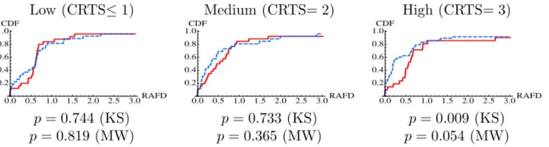
Figure 2 shows the distributions of RAF D1,1in the 6H (solid lines) and 1H5C (dashed

lines) treatments for three groups of subjects: low CRTS (left), medium CRTS (middle),

and high CRTS (right). While the distributions of RAF D1,1 for the two treatments

are not significantly diﬀerent for low and medium CRTS subjects, there is a significant

diﬀerence for high CRTS subjects.21 _{For high CRTS subjects, the median RAF D}

1,1

values are 0.570 in 6H and 0.183 in 1H5C. Thus, about 32% (0.183/0.570) of the median

Low (CRTS≤ 1) Medium (CRTS= 2) High (CRTS= 3)

0.0 0.5 1.0 1.5 2.0 2.5 3.0RAFD 0.2 0.4 0.6 0.8 1.0CDF 0.0 0.5 1.0 1.5 2.0 2.5 3.0RAFD 0.2 0.4 0.6 0.8 1.0CDF 0.0 0.5 1.0 1.5 2.0 2.5 3.0RAFD 0.2 0.4 0.6 0.8 1.0CDF p = 0.744 (KS) p = 0.733 (KS) p = 0.009 (KS) p = 0.819 (MW) p = 0.365 (MW) p = 0.054 (MW)

Fig. 2: Distributions of RAF D1,1 in 6H (solid lines) and 1H5C (dashed lines) for Low

(left), Medium (middle), and High (right) CRTS subjects.

(15)

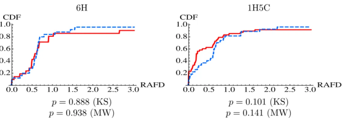
6H 1H5C 0.0 0.5 1.0 1.5 2.0 2.5 3.0RAFD 0.2 0.4 0.6 0.8 1.0CDF 0.0 0.5 1.0 1.5 2.0 2.5 3.0RAFD 0.2 0.4 0.6 0.8 1.0CDF p = 0.888 (KS) p = 0.101 (KS) p = 0.938 (MW) p = 0.141 (MW)

Fig. 3: Distributions of RAF D1,1 for High CRTS Subjects (solid lines) and Low CRTS

Subjects (dashed lines) in 6H (left) and 1H5C (right).

initial forecast deviation stems from individual bounded rationality, while the remaining 68% is due to strategic uncertainty for these subjects. Compared with the result based on all the data, the eﬀect of strategic uncertainty is much more pronounced for high CRTS subjects. For those with lower CRTSs, on the other hand, no significant eﬀect of strategic uncertainty is found.

It is quite clear from Figure 2 that the magnitude of RAF D in the 1H5C treatment is much smaller for high CRTS than low CRTS subjects. On the other hand, the magnitude of RAF D in the 6H treatment does not seem to vary across the three groups.

This is confirmed by Figure 3, which shows the distributions of RAF D1,1 for high

CRTS (solid lines) and low CRTS (dashed lines) subjects in the 6H (left) and 1H5C (right) treatments. We omitted medium CRTS subjects to focus on the two extreme groups. In the 6H treatment, the distributions of RAF D1,1for the two groups of subjects

are very similar, except for very high RAF D values, and are not significantly different. On the other hand, the two distributions appear to be quite different in the 1H5C treatment, although this difference is not statistically significant.

The insignificant diﬀerence between the two distributions of RAF D1,1 in the 6H

treatment22 shows that the total initial effects of bounded rationality and strategic un-certainty are not significantly different for these two groups of subjects, although the effect of confusion on low CRTS subjects is much larger as shown in the 1H5C treat-ment. It is as if the lack of confusion by less-confused subjects (high CRTS subjects)

22_{If anything, the distribution of RAF D}

1,1 for high CRTS subjects lies to the right of that for low

(16)

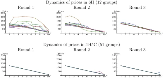
Dynamics of prices in 6H (12 groups)

Round 1 Round 2 Round 3

æ æ æ æ æ æ æ æ æ æ à à à à à à à à à à ì ì ì ì ì ì ì ì ì ì ò ò ò ò ò ò ò ò ò ò ô ô ô ô ô ô ô ô ô ô ç ç ç ç ç ç ç ç ç ç á á á á á á á á á á ó ó ó ó ó ó ó ó ó ó õ õ õ õ õ õ õ õ õ õ æ æ æ æ æ æ æ æ æ æ à à à à à à à à à à 1 2 3 4 5 6 7 8 9 10t 50 100 150 200 250Price æ æ æ æ æ æ æ æ æ æ à à à à à à à à à à ì ì ì ì ì ì ì ì ì ì ò ò ò ò ò ò ò ò ò ò ô ô ô ô ô ô ô ô ô ô ç ç ç ç ç ç ç ç ç ç á á á á á á á á á á ó ó ó ó ó ó ó ó ó ó õ õ õ õ õ õ õ õ õ õ æ æ æ æ æ æ æ æ æ æ à à à à à à à à à à 1 2 3 4 5 6 7 8 9 10t 50 100 150 200 250Price æ æ æ æ æ æ æ æ æ æ à à à à à à à à à à ì ì ì ì ì ì ì ì ì ì ò ò ò ò ò ò ò ò ò ò ô ô ô ô ô ô ô ô ô ô ç ç ç ç ç ç ç ç ç ç á á á á á á á á á á ó ó ó ó ó ó ó ó ó ó õ õ õ õ õ õ õ õ õ õ æ æ æ æ æ æ æ æ æ æ à à à à à à à à à à 1 2 3 4 5 6 7 8 9 10t 50 100 150 200 250Price

Dynamics of prices in 1H5C (51 groups)

Round 1 Round 2 Round 3

æ æ æ æ æ æ æ æ æ æ à à à à à à à à à à ì ì ì ì ì ì ì ì ì ì ò ò ò ò ò ò ò ò ò ò ô ô ô ô ô ô ô ô ô ô ç ç ç ç ç ç ç ç ç ç á á á á á á á á á á ó ó ó ó ó ó ó ó ó ó õ õ õ õ õ õ õ õ õ õ æ æ æ æ æ æ æ æ æ æ à à à à à à à à à à ì ì ì ì ì ì ì ì ì ì ò ò ò ò ò ò ò ò ò ò ô ô ô ô ô ô ô ô ô ô ç ç ç ç ç ç ç ç ç ç á á á á á á á á á á ó ó ó ó ó ó ó ó ó ó õ õ õ õ õ õ õ õ õ õ æ æ æ æ æ æ æ æ æ æ à à à à à à à à à à ì ì ì ì ì ì ì ì ì ì ò ò ò ò ò ò ò ò ò ò ô ô ô ô ô ô ô ô ô ô ç ç ç ç ç ç ç ç ç ç á á á á á á á á á á ó ó ó ó ó ó ó ó ó ó õ õ õ õ õ õ õ õ õ õ æ æ æ æ æ æ æ æ æ æ à à à à à à à à à à ì ì ì ì ì ì ì ì ì ì ò ò ò ò ò ò ò ò ò ò ô ô ô ô ô ô ô ô ô ô ç ç ç ç ç ç ç ç ç ç á á á á á á á á á á ó ó ó ó ó ó ó ó ó ó õ õ õ õ õ õ õ õ õ õ æ æ æ æ æ æ æ æ æ æ à à à à à à à à à à ì ì ì ì ì ì ì ì ì ì ò ò ò ò ò ò ò ò ò ò ô ô ô ô ô ô ô ô ô ô ç ç ç ç ç ç ç ç ç ç á á á á á á á á á á ó ó ó ó ó ó ó ó ó ó õ õ õ õ õ õ õ õ õ õ æ æ æ æ æ æ æ æ æ æ à à à à à à à à à à ì ì ì ì ì ì ì ì ì ì ò ò ò ò ò ò ò ò ò ò ô ô ô ô ô ô ô ô ô ô ç ç ç ç ç ç ç ç ç ç á á á á á á á á á á ó ó ó ó ó ó ó ó ó ó õ õ õ õ õ õ õ õ õ õ 1 2 3 4 5 6 7 8 9 10t 50 100 150 200 250Price æ æ æ æ æ æ æ æ æ æ à à à à à à à à à à ì ì ì ì ì ì ì ì ì ì ò ò ò ò ò ò ò ò ò ò ô ô ô ô ô ô ô ô ô ô ç ç ç ç ç ç ç ç ç ç á á á á á á á á á á ó ó ó ó ó ó ó ó ó ó õ õ õ õ õ õ õ õ õ õ æ æ æ æ æ æ æ æ æ æ à à à à à à à à à à ì ì ì ì ì ì ì ì ì ì ò ò ò ò ò ò ò ò ò ò ô ô ô ô ô ô ô ô ô ô ç ç ç ç ç ç ç ç ç ç á á á á á á á á á á ó ó ó ó ó ó ó ó ó ó õ õ õ õ õ õ õ õ õ õ æ æ æ æ æ æ æ æ æ æ à à à à à à à à à à ì ì ì ì ì ì ì ì ì ì ò ò ò ò ò ò ò ò ò ò ô ô ô ô ô ô ô ô ô ô ç ç ç ç ç ç ç ç ç ç á á á á á á á á á á ó ó ó ó ó ó ó ó ó ó õ õ õ õ õ õ õ õ õ õ æ æ æ æ æ æ æ æ æ æ à à à à à à à à à à ì ì ì ì ì ì ì ì ì ì ò ò ò ò ò ò ò ò ò ò ô ô ô ô ô ô ô ô ô ô ç ç ç ç ç ç ç ç ç ç á á á á á á á á á á ó ó ó ó ó ó ó ó ó ó õ õ õ õ õ õ õ õ õ õ æ æ æ æ æ æ æ æ æ æ à à à à à à à à à à ì ì ì ì ì ì ì ì ì ì ò ò ò ò ò ò ò ò ò ò ô ô ô ô ô ô ô ô ô ô ç ç ç ç ç ç ç ç ç ç á á á á á á á á á á ó ó ó ó ó ó ó ó ó ó õ õ õ õ õ õ õ õ õ õ æ æ æ æ æ æ æ æ æ æ à à à à à à à à à à ì ì ì ì ì ì ì ì ì ì ò ò ò ò ò ò ò ò ò ò ô ô ô ô ô ô ô ô ô ô ç ç ç ç ç ç ç ç ç ç á á á á á á á á á á ó ó ó ó ó ó ó ó ó ó õ õ õ õ õ õ õ õ õ õ 1 2 3 4 5 6 7 8 9 10t 50 100 150 200 250Price æ æ æ æ æ æ æ æ æ æ à à à à à à à à à à ì ì ì ì ì ì ì ì ì ì ò ò ò ò ò ò ò ò ò ò ô ô ô ô ô ô ô ô ô ô ç ç ç ç ç ç ç ç ç ç á á á á á á á á á á ó ó ó ó ó ó ó ó ó ó õ õ õ õ õ õ õ õ õ õ æ æ æ æ æ æ æ æ æ æ à à à à à à à à à à ì ì ì ì ì ì ì ì ì ì ò ò ò ò ò ò ò ò ò ò ô ô ô ô ô ô ô ô ô ô ç ç ç ç ç ç ç ç ç ç á á á á á á á á á á ó ó ó ó ó ó ó ó ó ó õ õ õ õ õ õ õ õ õ õ æ æ æ æ æ æ æ æ æ æ à à à à à à à à à à ì ì ì ì ì ì ì ì ì ì ò ò ò ò ò ò ò ò ò ò ô ô ô ô ô ô ô ô ô ô ç ç ç ç ç ç ç ç ç ç á á á á á á á á á á ó ó ó ó ó ó ó ó ó ó õ õ õ õ õ õ õ õ õ õ æ æ æ æ æ æ æ æ æ æ à à à à à à à à à à ì ì ì ì ì ì ì ì ì ì ò ò ò ò ò ò ò ò ò ò ô ô ô ô ô ô ô ô ô ô ç ç ç ç ç ç ç ç ç ç á á á á á á á á á á ó ó ó ó ó ó ó ó ó ó õ õ õ õ õ õ õ õ õ õ æ æ æ æ æ æ æ æ æ æ à à à à à à à à à à ì ì ì ì ì ì ì ì ì ì ò ò ò ò ò ò ò ò ò ò ô ô ô ô ô ô ô ô ô ô ç ç ç ç ç ç ç ç ç ç á á á á á á á á á á ó ó ó ó ó ó ó ó ó ó õ õ õ õ õ õ õ õ õ õ æ æ æ æ æ æ æ æ æ æ à à à à à à à à à à ì ì ì ì ì ì ì ì ì ì ò ò ò ò ò ò ò ò ò ò ô ô ô ô ô ô ô ô ô ô ç ç ç ç ç ç ç ç ç ç á á á á á á á á á á ó ó ó ó ó ó ó ó ó ó õ õ õ õ õ õ õ õ õ õ 1 2 3 4 5 6 7 8 9 10t 50 100 150 200 250Price

Fig. 4: Dynamics of Realised Prices in 6H (top) and 1H5C (bottom) for Three Rounds.

is compensated by their belief in the confusion of others (strategic uncertainty). This finding on the forecast deviations is very similar to the result of Cheung et al. (2014) who reported that the magnitude of mispricing was equally large in two market conditions: one where the subjects were not trained, and the other in which, despite being trained, the subjects were uncertain whether all the other subjects had been trained.23

2.3 Dynamics: Prices and Forecasts

Thus far, we have only considered the forecasts submitted before subjects observed any prices. In what way did subjects change their forecasts after observing the realised prices? To answer this question, we first summarise the realised price data and then move on to the dynamics of forecast deviations.24

23_{We are grateful to an anonymous referee for pointing out this similarity.}

24_{There was an error in the parameter settings of some of the 1H5C sessions, which resulted in four}

subjects and 20 computer traders interacting in one group instead of one subject and five computer traders. This error did not have any eﬀect on the initial forecast deviations (which is why we used all the data in the previous analysis). As for later rounds/periods, although subjects observed the same price dynamics as most of the others in cases without errors (prices following the fundamental value), the error may have had an impact on how a subject forecasted in a later round if the subject experienced outcomes that could not occur in the true setting. Such outcomes were either (1) a subject obtaining more than 24 units of stock, or (2) a subject submitting a buy order for more than the total availability

(QD ≥ 24 − number of stocks he has) and seeing the price strictly below what s/he had specified in

his/her order (P D). In the following analysis of the dynamics of forecast deviations, we omitted those subjects (six in total) in 1H5C who experienced such outcomes. Out of these six subjects, two had CRTS= 2 while the remaining four had CRTS= 3. For the price dynamics, we omitted all the data from sessions with an error, simply because the prices always followed the fundamental value in these sessions.

(17)

Round 1

Dynamics of median RAF Dt,1 Distribution of RAF D1,2i

1 2 3 4 5 6 7 8 9 10t 0.2 0.4 0.6 0.8 1.0RAFD 0.0 0.5 1.0 1.5 2.0 2.5 3.0RAFD 0.2 0.4 0.6 0.8 1.0 CDF p < 0.001 (KS, MW) Round 2

1 2 3 4 5 6 7 8 9 10t 0.2 0.4 0.6 0.8 1.0RAFD 0.0 0.5 1.0 1.5 2.0 2.5 3.0RAFD 0.2 0.4 0.6 0.8 1.0CDF p < 0.001 (KS, MW)

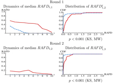
Fig. 5: Dynamics of the Median RAF Dt,r(left), and Distributions of RAF D1,r+1i (right)

in Period 1 of the Next Round for 1H5C (dashed lines) and 6H (solid lines) in Round 1 (top) and Round 2 (bottom).

Note: The p-values are given for two-tailed KS and MW tests. In conducting the statis-tical tests, for 6H we took the mean RAF D values for the six traders in the same group and used these as independent observations.

Figure 4 shows the dynamics of the realised prices over three rounds in 6H (top) and 1H5C (bottom). As expected, the prices in the 1H5C treatment followed the fundamental value except for a few rare cases in which a single human subject dominated one side of the market by placing a buy order with a large quantity at a price above the fundamental value (period 9 in round 2 and period 10 in round 3). In the 6H treatment, on the other hand, prices deviated from the fundamental value in round 1. Such deviations of prices from the fundamental value gradually disappeared in rounds 2 and 3 as subjects gained experience from trading in the same market environment with a group of subjects as reported in the literature.

Next, we turn to the dynamics of the forecast deviation. How quickly did subjects in 1H5C learn to forecast prices to follow the fundamental value? What about the subjects

in 6H? The left panel of Figure 5 shows the dynamics of the median RAF Dt,r over 10

periods in rounds 1 (top) and 2 (bottom). It is clear that the subjects in 1H5C (dashed lines) learned much more quickly than those in 6H (solid lines) to forecast prices that

(18)

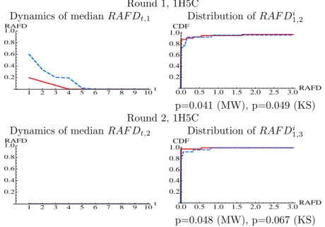
Round 1, 1H5C

1 2 3 4 5 6 7 8 9 10t 0.2 0.4 0.6 0.8 1.0RAFD 0.0 0.5 1.0 1.5 2.0 2.5 3.0RAFD 0.2 0.4 0.6 0.8 1.0 CDF p=0.041 (MW), p=0.049 (KS) Round 2, 1H5C

1 2 3 4 5 6 7 8 9 10t 0.2 0.4 0.6 0.8 1.0RAFD 0.0 0.5 1.0 1.5 2.0 2.5 3.0RAFD 0.2 0.4 0.6 0.8 1.0 CDF p=0.048 (MW), p=0.067 (KS)

in Period 1 of the Next Round for Low CRTS (dashed lines) and High CRTS (solid lines) Subjects in Round 1 (top) and Round 2 (bottom) in 1H5C.

followed the fundamental value. As can be seen in the right panel of the figure, by the beginning of round 2 (3), close to 80 % (90%) of the subjects in the 1H5C treatment (dashed lines) had RAF D = 0, whereas this was not the case for subjects in the 6H treatment (solid lines). These diﬀerences, however, are quite natural given the diﬀerences in the realised prices in the two treatments. As shown in Figure 4, while subjects in the 1H5C treatment saw prices that were exactly the same as the fundamental value in every period, those in the 6H treatment saw prices that deviated greatly from it.

What about the similarities (in 6H) and diﬀerences (in 1H5C) of initial RAF D be-tween high and low CRTS groups observed above? Did they disappear or persist once subjects in a market observed the same prices and started learning?

We start with the diﬀerences in initial RAF D between the two extreme CRTS groups in 1H5C. Given the dynamics of the median RAF D in 1H5C treatments, one could easily imagine that the initial diﬀerence between the two CRTS groups would disappear quickly in this treatment. Figure 6 shows that this was indeed the case.25

What about the initial similarities of RAF D between high and low CRTS groups in

25_{Although the diﬀerences between the distributions of RAFD for the two extreme CRTS groups at}

(19)

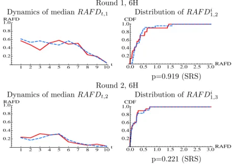
Round 1, 6H

1 2 3 4 5 6 7 8 9 10t 0.2 0.4 0.6 0.8 1.0RAFD 0.0 0.5 1.0 1.5 2.0 2.5 3.0RAFD 0.2 0.4 0.6 0.8 1.0 CDF p=0.919 (SRS) Round 2, 6H

1 2 3 4 5 6 7 8 9 10t 0.2 0.4 0.6 0.8 1.0RAFD 0.0 0.5 1.0 1.5 2.0 2.5 3.0RAFD 0.2 0.4 0.6 0.8 1.0 CDF p=0.221 (SRS)

in Period 1 of the Next Round for Low CRTS (dashed lines) and High CRTS (solid lines) Subjects in Round 1 (top) and Round 2 (bottom) in 6H.

Note: We tested whether the within-group diﬀerences between the average RAFD values of the two groups of subjects diﬀer from zero (two-tailed signed rank-sum (SRS) test).

the 6H treatment? Did they persist or did they disappear as subjects started learning? Figure 7 shows that the RAF D values of these two CRTS groups continued to be similar in later periods and rounds.

By comparing the right panels in Figures 6 and 7, it can easily be seen that the distributions of RAF D for the 1H5C and 6H treatments at the beginning of rounds 2 and 3 are significantly diﬀerent for both low and high CRTS groups.

We interpret these convergences of RAFDs among CRTS groups in each treatment as being the result of subjects’ adaptive learning based on commonly observed prices. This has been demonstrated by Haruvy et al. (2007) in the context of a similar asset market experiment, and by Hommes et al. (2005), Heemeijer et al. (2009), Bao et al. (2012), and Anufriev and Hommes (2012) in the context of diﬀerent price-forecasting experiments.

(20)

3 Conclusion

In this paper, we investigated to what extent forecast deviations in experimental asset markets are caused by individual bounded rationality (or confusion) and by strategic uncertainty (uncertainty about others’ behaviour) to better understand the source of mispricing in these experimental markets. We compared the initial price forecasts sub-mitted by subjects in two market environments: one in which all six traders were human subjects (6H), and the other where one human interacted with five computer traders whose behaviour was known (1H5C).

Our analysis shows that about 50% of the median initial forecast deviation is due to confusion and the remaining 50% is due to strategic uncertainty. We also found that the eﬀect of strategic uncertainty is greater for those subjects with a higher cognitive ability that manifests as a higher score in the CRT (Frederick, 2005). For those with a perfect CRT score, individual bounded rationality accounts for about 30%, while strate-gic uncertainty accounts for the remaining 70% of the median initial forecast deviation from the fundamental value. For those with lower CRT scores, we did not observe any significant eﬀect of strategic uncertainty.

Our results show that both strategic uncertainty and individual bounded rationality (or confusion) have significant power in explaining the initial forecast deviations. While confusion clearly plays an important role in causing mispricing in these experimental asset markets as recently emphasised by Huber and Kirchler (2012) and Kirchler et al. (2012), so too does strategic uncertainty as conjectured by Smith et al. (1988) and recently demonstrated by Cheung et al. (2014). Subjects being confused cannot be the whole story behind the bubble.

Cheung et al. (2014) reported very similar findings to ours regarding the eﬀect of confusion and strategic uncertainty despite a number of diﬀerences in (a) the experi-mental setup, (b) key experiexperi-mental manipulation, and (c) data investigated (i.e., ob-served/forecasted prices). Both our results and those of Cheung et al. (2014) point to the importance of (1) better understanding of how subjects with varying degrees of “confusion” form their beliefs of others, and (2) how such heterogeneity leads to varying behaviour among subjects in these markets. Addressing these issues is left for future

(21)

research.

We make one final remark before closing the paper. It is quite well known that experiences in trading in the same market environment help subjects “learn” to trade at prices closer to the fundamental value and to forecast prices accordingly. We have seen that diﬀerences in forecast deviations among CRTS groups disappear in 1H5C, whereas their similarities persists in 6H treatments. We interpret these outcomes as being the result of subjects learning adaptively based on commonly observed prices. What happens if the common experience among subjects is broken owing to the inflow of new and inexperienced subjects or changes in the market environments? Hussam et al. (2008) and Deck et al. (2014) showed that these changes can re-generate large mispricing, but both articles remain silent as to the relative eﬀects of the post-shock confusion and strategic uncertainty that caused such mispricing to re-emerge. We believe this is also an interesting issue to investigate, and have taken a step toward addressing it in Akiyama

et al. (2014).

Faculty of Engineering, Information and Systems, University of Tsukuba.

Aix-Marseille University (Aix-Marseille School of Economics), CNRS & EHESS, and IUF.

Faculty of Engineering, Information and Systems, University of Tsukuba.

References

Akiyama, E., Hanaki, N. and Ishikawa, R. (2014). ‘How do experienced traders respond to inflows of inexperienced traders? an experimental analysis’, Journal of Economic

Dynamics and Control, vol. 45, pp. 1–18.

Anufriev, M. and Hommes, C. (2012). ‘Evolutionary selection of individual expectations and aggregate outcomes in asset pricing experiments’, American Economics Journal,

Microeconomics, vol. 4(4), pp. 35–64.

Bao, T., Hommes, C., Sonnemans, J. and Tuinstra, J. (2012). ‘Individual expectations, limited rationality and aggregate outcomes’, Journal of Economic Dynamics and

(22)

Brañas-Garza, P., Garc´ıa-Muñoz, T. and Hernán, R. (2012). ‘Cognitive effort in the beauty contest game’, Journal of Economic Behavior and Organization, vol. 83(2), pp. 254–260.

Breaban, A. and Noussair, C.N. (2014). ‘Fundamental value trajectories and trader char-acteristics in an asset market experiment’, University of Jaume I and Tilburg Univer-sity.

Camerer, C.F. (2003). Behavioral Game Theory: Experiments in Strategic Interaction, New York: Russell Sage Foundation.

Cason, T.N. and Friedman, D. (1997). ‘Price formation in single call markets’,

Econo-metrica, vol. 65(2), pp. 311–345.

Cheung, S.L., Hedegaard, M. and Palan, S. (2014). ‘To see is to believe: Common expectations in experimental asset markets’, European Economic Review, vol. 66, pp. 84–96.

Corgnet, B., Gonzalez, R.H., Kujal, P. and Porter, D. (2014). ‘The eﬀect of earned vs. house money on price bubble formation in experimental asset markets’, forthcoming in Review of Finance. doi: 10.1093/rof/rfu031.

Costa-Gomes, M.A. and Crawford, V.P. (2006). ‘Cognition and behavior in two-person guessing games: An experimental study’, American Economic Review, vol. 96(5), pp. 1737–1768.

Crawford, V.P., Costa-Gomes, M.A. and Iriberri, N. (2013). ‘Structural models of nonequilibrium strategic thinking: Theory, evidence, and applications’, Journal of

Economic Literature, vol. 51(1), pp. 5–62.

Deck, C., Porter, D. and Smith, V. (2014). ‘Double bubbles in assets markets with multiple generations’, Journal of Behavioral Finance, vol. 15(2), pp. 79–88.

Fehr, E. and Tyran, J.R. (2001). ‘Does money illusion matter?’, American Economic

Review, vol. 91(5), pp. 1239–1262.

Fehr, E. and Tyran, J.R. (2005). ‘Individual irrationality and aggregate outcomes’,

(23)

Fehr, E. and Tyran, J.R. (2008). ‘Limited rationality and strategic interaction: The impact of the strategic environment on nominal inertia’, Econometrica, vol. 76(2), pp. 353–394.

Fischbacher, U. (2007). ‘z-tree: Zurich toolbox for ready-made economic experiments’,

Experimental Economics, vol. 10(2), pp. 171–178.

Frederick, S. (2005). ‘Cognitive reflection and decision making’, Journal of Economic

Perspectives, vol. 19(4), pp. 25–42.

Haltiwanger, J. and Waldman, M. (1985). ‘Rational expectations and the limits of ra-tionality: An analysis of heterogeneity’, American Economics Review, vol. 75(3), pp. 326–340.

Haltiwanger, J. and Waldman, M. (1989). ‘Limited rationality and strategic comple-ments: The implications for macroeconomics’, Quarterly Journal of Economics, vol. 104, pp. 463–484.

Haruvy, E., Lahav, Y. and Noussair, C.N. (2007). ‘Traders’ expectations in asset markets: Experimental evidence’, American Economics Review, vol. 97(5), pp. 1901–1920. Heemeijer, P., Hommes, C., Sonnemans, J. and Tuinstra, J. (2009). ‘Price stability and

volatility in markets with positive and negative expectations feedback: An experimen-tal investigation’, Journal of Economic Dynamics and Control, vol. 33, pp. 1052–1072. Ho, T.H., Camerer, C. and Weigelt, K. (1998). ‘Iterated dominance and iterated best response in experimental “p-beauty contests”’, American Economic Review, vol. 88(4), pp. 947–969.

Hommes, C., Sonnemans, J., Tuinstra, J. and van de Velden, H. (2005). ‘Coordination of expectations in asset pricing experiments’, Review of Financial Studies, vol. 18(3), pp. 955–980.

Houser, D. and Kurzban, R. (2002). ‘Revisiting kindness and confusion in public goods experiments’, American Economic Review, vol. 92(4), pp. 1062–1069.

(24)

Huber, J. and Kirchler, M. (2012). ‘The impact of instructions and procedure on reduc-ing confusion and bubbles in experimental asset markets’, Experimental Economics, vol. 15, pp. 89–105.

Hussam, R.N., Porter, D. and Smith, V.L. (2008). ‘Thar she blows: Can bubbles be rekindled with experienced subjects?’, American Economic Review, vol. 98, pp. 927– 934.

Johnson, E.J., Camerer, C., Sen, S. and Rymon, T. (2002). ‘Detecting failures of back-ward induction: Monitoring information search in sequential bargaining’, Journal of

Economic Theory, vol. 104, pp. 16–47.

Kirchler, M., Huber, J. and St¨ockl, T. (2012). ‘Thar she bursts: Reducing confusion reduces bubbles’, American Economic Review, vol. 102(2), pp. 865–883.

Lei, V., Noussair, C.N. and Plott, C.R. (2001). ‘Nonspeculative bubbles in experimen-tal asset markets: Lack of common knowledge of rationality vs. actual irrationality’,

Econometrica, vol. 69, pp. 831–859.

Nagel, R. (1995). ‘Unraveling in guessing games: An experimental study’, American

Economics Review, vol. 85(5), pp. 1313–1326.

Noussair, C., Robin, S. and Ruﬃeux, B. (2001). ‘Price bubbles in laboratory asset mar-kets with constant fundamental values’, Experimental Economics, vol. 4, pp. 87–105. Oechssler, J., Roider, A. and Schmitz, P.W. (2009). ‘Cognitive abilities and behavioral

biases’, Journal of Economic Behavior and Organization, vol. 72, pp. 147–152. Palan, S. (2013). ‘A review of bubbles and crashes in experimental asset markets’, Journal

of Economic Surveys, vol. 27(3), pp. 570–588.

Porter, D.P. and Smith, V.L. (1995). ‘Futures contracting and dividend uncertainty in experimental asset markets’, The Journal of Business, vol. 68(4), pp. 509–541. Smith, V.L., Suchanek, G.L. and Williams, A.W. (1988). ‘Bubbles, crashes, and

en-dogenous expectations in experimental spot asset markets’, Econometrica, vol. 56, pp. 1119–1151.

(25)

St¨ockl, T., Huber, J. and Kirchler, M. (2010). ‘Bubble measures in experimental asset markets’, Experimental Economics, vol. 13, pp. 284–298.

Sutan, A. and Willinger, M. (2009). ‘Guessing with negative feedback: An experiment’,

Journal of Economic Dynamics and Control, vol. 33, pp. 1123–1133.

van Boening, M.V., Williams, A.W. and LaMaster, S. (1993). ‘Price bubbles and crashes in experimental call markets’, Economics Letters, vol. 41, pp. 179–185.

(26)

Appendix A. Table of fundamental values given to

the subjects

No. of remaining periods Dividend Next value

At the end of period 1 9 12 108

Next value before the beginning of period 1 is 120.