HAL Id: hal-03132361
https://hal.archives-ouvertes.fr/hal-03132361
Submitted on 5 Feb 2021
HAL is a multi-disciplinary open access
archive for the deposit and dissemination of
sci-entific research documents, whether they are
pub-lished or not. The documents may come from
teaching and research institutions in France or
abroad, or from public or private research centers.
L’archive ouverte pluridisciplinaire HAL, est
destinée au dépôt et à la diffusion de documents
scientifiques de niveau recherche, publiés ou non,
émanant des établissements d’enseignement et de
recherche français ou étrangers, des laboratoires
publics ou privés.
Influence the Community of Non-native Species Within
Them
Kathrin Holenstein, William Simonson, Kevin Smith, Tim Blackburn, Anne
Charpentier
To cite this version:
Kathrin Holenstein, William Simonson, Kevin Smith, Tim Blackburn, Anne Charpentier. Non-native
Species Surrounding Protected Areas Influence the Community of Non-native Species Within Them.
Frontiers in Ecology and Evolution, Frontiers Media S.A, 2021, 8, �10.3389/fevo.2020.625137�.
�hal-03132361�
Edited by: Ana Novoa, Institute of Botany (ASCR), Czechia Reviewed by: Desika Moodley, Academy of Sciences of the Czech Republic (ASCR), Czechia Belinda Gallardo, Pyrenean Institute of Ecology, Spain *Correspondence: Kathrin Holenstein [email protected]
Specialty section: This article was submitted to Biogeography and Macroecology, a section of the journal Frontiers in Ecology and Evolution Received: 02 November 2020 Accepted: 09 December 2020 Published: 08 January 2021 Citation: Holenstein K, Simonson WD, Smith KG, Blackburn TM and Charpentier A (2021) Non-native Species Surrounding Protected Areas Influence the Community of Non-native Species Within Them. Front. Ecol. Evol. 8:625137. doi: 10.3389/fevo.2020.625137
Non-native Species Surrounding
Protected Areas Influence the
Community of Non-native Species
Within Them
Kathrin Holenstein1*, William D. Simonson2, Kevin G. Smith3, Tim M. Blackburn4,5and
Anne Charpentier1
1CEFE, Univ. Montpellier, CNRS, EPHE, IRD, Univ. Paul Valéry Montpellier 3, Montpellier, France,2UN Environment
Programme World Conservation Monitoring Centre, UNEP-WCMC, Cambridge, United Kingdom,3International Union for
Conservation of Nature Global Species Programme, Cambridge, United Kingdom,4Department of Genetics, Evolution and
Environment, Centre for Biodiversity and Environment Research, University College London, London, United Kingdom,
5Institute of Zoology, Zoological Society of London, London, United Kingdom
Protected areas (PAs) are a key element of global conservation strategies aiming to protect habitats and species from various threats such as non-natives species (NNS) with negative ecological impacts. Yet little is known about the mechanisms by which PAs are colonized by NNS, and more specifically the role of colonizing events from surrounding areas. Here, we compared terrestrial and freshwater non-native plants and animals recorded in Norwegian PAs and in 5-km belts around them, using the database of the Norwegian Biodiversity Information Centre Species Map Service. Our analysis included 1,602 NNS and 671 PAs. We found that NNS were recorded in only 23% of the PAs, despite the fact that 90% of the 5-km belts were colonized by at least one NNS. A Zero-inflated negative binomial regression model showed that the number of NNS in the 5-km belts was a strong explanatory variable of the NNS richness inside PAs. Other significant variables included the surface area of the PA, mean human population density in the PA, main type of habitat and accessibility of PAs. We also observed similarity in the species in and around the PAs, with, on average, two thirds of the NNS present in a specific PA also present in its 5-km belt. Furthermore, NNS were recorded in PAs on average 4.5 years after being recorded in the 0–5 km belts, suggesting a dynamic of rapid colonization from the belts to the PAs. Invasive NNS represented 12% of NNS in the belts but 40% in the PAs. This difference was related to the higher abundance of invasive NNS in the belts. Our results highlight the necessity of expanding the focus of NNS management in PAs beyond their boundaries, in particular to prevent incursions of NNS with high negative ecological impact.
Keywords: protected areas, non-native species, alien species, protected area boundaries, invasive species, species distribution
INTRODUCTION
Protected areas (PAs) are key target elements of global biodiversity conservation strategies. In 2010, 150 governmental leaders committed, through the Aichi Target 11 in the Convention on Biological Diversity, to improve the status of biodiversity by setting 17% of the global terrestrial area under protection by 2020 (CBD, 2020). The main purposes of PAs are to maintain natural ecosystem functioning, prevent habitat degradation due to human activities (Rodrigues et al., 2004), conserve biodiversity (Worboys, 2015) and protect nature from various threats (Mathur et al., 2015) such as acting as natural filters against invasive non-native species (Foxcroft et al., 2011).
According to IUCN, a non-native species (NNS) is a species introduced outside its natural past or present distribution (IUCN, 2016). During the last two centuries the number of introduced NNS species has increased substantially worldwide with no sign of saturation (Seebens et al., 2017a). Their spread is a consequence of increased human mobility, and the expansion and globalization of trade between countries and continents (Nunes et al., 2015; Chapman et al., 2017; Seebens et al., 2018; Ward et al., 2020). Although the ecological impacts of most NNS are either negligible or unknown (Jari´c and Cvijanovi´c, 2012; Seebens et al., 2018; Blackburn et al., 2019), some non-natives are invasive, or potentially invasive: i.e., they have negative impacts on the recipient species and ecosystem (IUCN, 2016; Blackburn et al., 2019). Biological invasions are one of the leading causes of global biodiversity loss (Intergovernmental science-policy platform on biodiversity ecosystem services, 2019) and are one of the principal drivers of recent species extinctions (Clavero and García-Berthou, 2005; Bellard et al., 2016; Blackburn et al., 2019).
Numerous guidelines and technical tools have been developed to assist in the management of invasive NNS in PAs (e.g.,
de Pooter et al., 2007; Monaco and Genovesi, 2014). These manuals generally advocate the early detection and eradication of all NNS, including those that have not been proven to be invasive, as an implementation of a precautionary approach that considers all NNS to be potentially invasive (McNeely et al., 2001; Monaco and Genovesi, 2014). Beyond the threat to biodiversity posed by invasive species, all NNS represent a human footprint on natural environments. NNS introduced by humans are considered undesirable in PAs, the purpose of which is to preserve nature in as pristine a state as possible (Hettinger, 2001). The presence of NNS also potentially contributes to increasing homogenization of native biological communities (McKinney and Lockwood, 1999; Lambdon et al., 2008; Kortz and Magurran, 2019).
Previous studies have shown that NNS richness patterns within PAs are linked to anthropogenic factors such as road networks and human population density inside PAs (Spear et al., 2013; Dimitrakopoulos et al., 2017; Gallardo et al., 2017; Moustakas et al., 2018). Other properties of the PAs, such as their surface area and protection status, also influence NNS richness (Gallardo et al., 2017; Liu et al., 2020). Furthermore, NNS presence in PAs is also driven by the properties of the surrounding areas, including human land use, human population
density and road density (Foxcroft et al., 2011; Spear et al., 2013). These results suggest that, even if long-distance dispersal can be important for the expansion of NNS, especially in the early stages (Ramakrishnan et al., 2010), short-distance dispersal represents a significant contribution to their colonization dynamics. One of the few documented examples was published recently byLiu et al. (2020), based on the global alien distributions of 894 animal species: they found that 89–99% of PAs had an established population of at least one of these species within 10–100 km of their boundaries, but the majority of PAs were not colonized by any of them. Nevertheless, little is known about the influence of the NNS pool present in close proximity to PAs on the NNS communities within them (but for an example seeMeiners and Pickett, 2013).
Here, we analyze the composition of terrestrial and freshwater non-native plants and animals present in Norwegian PAs, and in belts of 0–5, 5–10, and 10–20 km around them, to assess the extent to which the community of NNS in areas immediately surrounding PAs relates to NNS within PAs. We selected Norway due to the availability of an extensive database on NNS from the Norwegian Biodiversity Information Centre (NBIC) and the Global Biodiversity Information Facility Norway (GBIF Norway). We hypothesized that the presence of NNS in PAs should mainly be a result of colonization from surrounding areas. NNS in close proximity to PAs should thus influence the community of NNS present in PAs qualitatively, quantitatively and temporally. We expected to find:
1. A high proportion of NNS present in a PA are also present in its surroundings (qualitative similarity). The NNS in a PA will have taxonomic and ecological similarities to the pool of NNS in its surroundings. However, since invasive NNS are expected to have a higher colonization potential than non-invasive NNS, invasives should be present in higher proportions inside PAs than outside in comparison to other NNS.
2. The total number of NNS present inside a PA is a positive function of the richness of NNS in its surroundings (quantitative influence). In addition, the most abundant species in the surroundings of PAs are more likely to be present within the PAs.
3. NNS are recorded in the areas surrounding PAs earlier than inside the PAs (temporal sequence).
METHODS
Data on Non-native Species
We downloaded NNS data from the NBIC Species Map Service (https://www.artskart.artsdatabanken.no, 10/04/2020. Data from: List supplementary material. Downloaded through the Species Map service). This database is provided by various contributors including research institutes, environmental agencies and NGOs. Biodiversity data from online databases are potentially biased, for example by accessibility of sites, lack of coverage of geographic and environmental variation that cover species distributions (Hortal et al., 2007), or by taxonomy, such as societal preferences in citizen science projects (Troudet et al., 2017). However, we consider the Norwegian database as one
of the most robust that is available, as it contains an extensive collection and evaluation of NNS from a wide range of taxa and across the country (Sandvik et al., 2019; Tsiamis et al., 2019).
We selected terrestrial and freshwater NNS records of the Kingdom “Animalia” and “Plantae” with an accuracy of <= 100 m. For this purpose, we retained only those species with the following habitat categories assigned by Norwegian Biodiversity Information Center (NBIC, https://www.biodiversity.no): terrestrial, limnic/terrestrial, limnic/marine habitats. We filtered for records from the year 1950 to the present. After selection, our NNS database included a total of 350,286 records of 1,602 species representing 21 different taxonomic classes. 14.9% of the NNS were animals and 85.1% were plants.
In order to consider potential ecological impacts caused by NNS, we used the ecological risk assessment conducted by the Norwegian Biodiversity Information Centre, in which each NNS is assigned to one of the following categories:
- “Severe impact” (SE): NNS with actual or potential ecologically harmful impact and the potential to become established across large areas;
- “High impact” (HI): NNS with either a moderate ability to spread but which cause at least a medium ecological effect, or have a minor ecological effect but have a high invasion potential;
- “Potentially high impact” (PH): NNS with either a high ecological effect and low invasion potential or high invasion potential without known ecological effect;
- “Low impact” (LO): NNS with no substantial impact upon Norwegian nature
- “Not known impact” (NK): NNS with no known impact; - “Not risk assessed” (NR): NNS not yet risk assessed.
NNS belonging to “Severe impact” and “High impact” categories are included in the Norwegian Black List 2012 of Alien Species. In total, 60% of the NNS included in the analysis were risk assessed, while 40% were not.
Data on Protected Areas
We extracted the shape files and information on the designation year and surface area of Norwegian PAs from the World Data Base on Protected Areas (WDPA, UNEP-WCMC and IUCN, 2019). The WDPA contains 3,143 registered Norwegian PAs of which 2,178 PAs are terrestrial and cover 54,749 km² of the land area of Norway (http://protectedplanet.net, accessed March 2020). We selected for analysis PAs with status “designated” and categorized as “terrestrial,” excluding “marine,” and “coastal” PAs. There are also PAs that are not assigned to any management categories (i.e., category marked as not assigned, not reported, not applicable); these PAs were excluded.
Protected areas of the WDPA are categorized in different International Union for Conservation of Nature (IUCN) categories, which range from category I (strictly protected or large, unmodified or slightly modified areas) to VI (protected areas with sustainable use of natural resources) whilst further PAs that are not assigned, not reported and not applicable (IUCN, https://www.iucn.org). For our study we selected PAs in category I, II (national parks) and IV (habitat/species management areas)
with a surface area >= 1 km². Since our analysis investigated NNS in PAs and belt zones up to a distance of 20 km around the PAs (see below), we also excluded PAs whose belt zones crossed the political borders with Sweden, Finland and Russia.
Applying these filters resulted in 671 PAs in our analysis: 623 PAs of IUCN category I (average surface area = 7.8 km²), 18 PAs of IUCN category II (average surface area = 1,064.9 km²) and 30 PAs of IUCN category IV (average surface area = 142.3 km²). All PAs were designated between 1959 and 2017 and had areas ranging between 1 and 3,444.8 km² (average 42.2 km²). They covered 28,314.9 km², which is 49.5% of the total terrestrial protected area of Norway.
Belt Zones Around Protected Areas
We mapped belt zones of 0–5, 5–10, and 10–20 km circumjacent to PAs using QGIS (http://qgis.osgeo.org, version 3.4.2-Madeira) (Figure 1). All PAs and belt zones were entirely within Norway. Where the belt zone of a PA included part or all of another PA, the intersecting area was not excluded from the belt, such that belts should not be considered as indicators of the state of protection. Our analysis focused on the belt of 0–5 km (henceforth referred to as 5-km belt) to investigate whether the composition of NNS communities within PAs was influenced by NNS in the immediate vicinity of PAs. The surface area of this belt naturally varied with the size of the PA, with a range 99.1–2,218.2 km² (average 167.7 km²).
Statistical Analysis
All analyses were performed using the statistical analysis tool R [R Core Team (2019), https://www.R-project.org, version 4.2.0]. We extracted NNS records for all the PAs and their belts, deriving from this a list of NNS for each PA and its surrounding belt. To test qualitative similarity, we used tests across all PAs and belts (i.e., overall comparisons considering independently the records made in a PA and in 5-km belts). The temporal sequence analysis was based on data where the NNS was present in the PA and the associated belts using a pairwise comparison. To test for quantitative influence, we used a mixture of tests considering data in PAs and their associated belts as independent (tests on abundance) or as paired for the other analysis (NNS present in PAs and associated 5-km belts and modeling NNS richness). Qualitative Similarity
Taxonomy and Ecological Impact
We compared the proportions of taxonomic classes and ecological impact categories of NNS between the PAs and belts using Pearson’s chi-squared tests.
Most Frequent NNS
To identify the most frequent NNS in the PAs, we selected NNS that were present in at least ten PAs. We compared them with the same number of NNS that were most frequent in the 5-km belts. Quantitative Influence
NNS Abundance
We defined the abundance of a species in a PA or a belt as the number of records of this species. The mean abundance of a
FIGURE 1 | Left: Map of Norway with protected areas (PAs) and belt zones, with an example of part of the network (detail shown in inset). Right: An example (Møysalen National Park) showing the area of the PA, the three belts of 0–5, 5–10, and 10–20 km distance from the PA boundary, and the locations of records of non-native animal and plant species.
species is therefore the number of records divided by the number of PAs or belts where it was present.
For NNS present in both the PAs and the 5-km belts, we tested if there was a correlation between their mean abundance in the PAs and the belt using a Spearman’s rank correlation (rho).
To test whether the NNS present in the PAs are among the most abundant in the 5-km belts, we compared the mean abundance of NNS present in both the PAs and the belts with the mean abundance of NNS present only in the belts using a Wilcoxon Rank Sum Test.
To test whether NNS of the impact categories “Severe impact” and “High impact” (black listed NNS) were more abundant in the 5-km belts than NNS of less severe impact categories (non-black listed NNS), we compared the mean abundance of these two groups of NNS in the 5-km belts using a Wilcoxon Rank Sum Test.
NNS Present in PAs and Associated 5-km Belts
To investigate the hypothesis that the presence of NNS in PAs is mainly a result of colonizing events from surrounding areas, we calculated, for each NNS present in the 5-km belts, the proportion of times it was present in both the belt and its associated PA, and the proportion of times it was present only in the 5-km belt but not in its associated PA. We then calculated the mean of these proportions for all the NNS present in the 5-km belts.
We applied the same approach for the NNS present in the PAs. We calculated the proportion of time they were present in both the PA and its associated 5-km belt, and the proportion of time they were present only in the PA but not in its associated 5-km belt. We then calculated the mean of these proportions for all the NNS present in the PAs.
Modeling NNS Richness
We selected five explanatory variables to model NNS richness in PAs, comprising two biotic variables (the most abundant land cover in the PAs and NNS richness in the 5-km belts); two anthropogenic variables (mean human population density of the region in which the PA is located and their accessibility), and PA surface area. Land cover was obtained from Copernicus Land Monitoring Service using information Label 1 (CLC, 2018). Label 1 information consists of five categories: “Artificial surfaces”, “Agricultural areas”, “Forest” and semi natural areas”, “Wetlands” and “Water bodies”. We extracted the land cover of each PA in QGIS and calculated the percentage of the most abundant land cover category in each PA.
NNS richness in each of the PAs and their associated 5-km belt zones was extracted from the NNS lists. The mean accessibility of PAs, calculated as the mean travel time from within PAs to the nearest city with a population >50,000 inhabitants, was extracted fromNelson (2008), a map integrating transportation networks and agglomeration index (a measure of urban concentration) and was downloaded from the European Commission (https://forobs. jrc.ec.europa.eu). Mean human population density was obtained fromWorldPop (2018). The surface areas of the PAs were filtered from the World Database of Protected Areas (WDPA, https:// protectedplanet.net). We assessed the relationships between predictor variables using Spearman’s Rank correlation. All predictors were retained for the analysis since they had little correlation among them (Supplementary Figure 1).
We applied a Zero-inflated Negative Binomial regression model with Poisson distribution (ZINB, Lawal, 2012) to test if the NNS richness in PAs is a result of the NNS richness in the associated 5-km belts, anthropogenic and PA properties. We assumed that if NNS have the opportunity to colonize PAs their richness inside is between 0 or higher and therefore is
a count process (Gallardo et al., 2017). On the other hand, for PAs that were uncolonized by NNS, we assumed this was due to missing vectors, distance, or the PA not having suitable habitat (Gallardo et al., 2017). The only outcome in this case is zero. The ZINB model consists of two parts: The first part is the negative binomial regression model, which explains the relationship between conditional variance and conditional mean compared to the Poisson distribution model. The second part, the binary distribution model, captures the excess of zero values that exceed the predicted zeros by the negative binomial distribution. We used the package “pscl” to run the ZINB (Achim et al., 2008; Jackman, 2020).
Temporal Sequence
Year of First Record in PAs and Associated Belts
To test whether NNS were recorded earlier in the surrounding belt than inside PAs, we extracted the years of first record for each NNS in the PAs and the 0–5, 5–10, and 10–20 km belt zones. We selected only NNS present in PAs. For each NNS we looked at the PA and the associated belts. We compared the years of first record in PAs and their three associated belts using a Kruskal-Wallis and Dunn’s test for pairwise comparison with the “fdr” adjustment method.
RESULTS
We analyzed 671 Norwegian PAs, of which only 22.8% were colonized by any NNS. In contrast, at least one NNS was present in 89.5% of the 5-km belts. The total number of NNS records was 8,641 in PAs, and 156,736 in the 5-km belts, which represents 2.4 and 44.7%, respectively, of all the Norwegian NNS records included in the analysis. The remaining records were in the 5– 10 km belts and 10–20 km belts or outside of them. The number of NNS was between 0 and 53 in PAs (mean = 0.87, SD = 3.68) and 0 and 440 (mean = 23.3, SD = 50.62) in 5-km belts. Of the 1,602 NNS in our analysis, 196 were present in the PAs, and 1,123 in the 5-km belts. All bar one of the 196 NNS present in the PAs (99.5%) were among the NNS present in the 5-km belts, the exception being the plant, Leucanthemum maximum. The number of NNS present in PAs also varied between IUCN categories (category I: mean ± SD = 0.68 ± 2.85; category II: 1.27 ± 2.35; category IV: 4.53 ± 11.03).
Qualitative Similarity
Taxonomy
More than 75% of the NNS in both the PAs and the 5-km belts were plants, although the proportion of plants was lower in PAs than in 5-km belts (Figure 2A). Five plant classes were present in the PAs vs. eight in the 5-km belts (Figure 2B). Eudicots (e.g., broadleaf trees Acer pseudoplatanus and Sambucus racemosa) represented the highest proportion in both the PAs and the 5-km belts but the proportion was significantly lower in the PAs than in the 5-km belts (Figure 2B). The inverse relationship was observed for Pinopsida (e.g., coniferous trees Picea stichensis and Abies alba), with a higher proportion of Pinopsida present in PAs. Non-native animal species represented 22% and 13% of the NNS in PAs and 5-km belts, respectively. Six animal classes were
present in the PAs and 8 in the 5-km belts, of which Insecta (e.g., the beetles Acrotrichis insularis and Cartodere nodifer) showed the highest proportion in PAs and 5-km belts, followed by Aves (e.g., the Canada goose Branta canadensis and the Mandarin duck Aix galericulata), with a significant higher proportion of Aves in PAs (Figure 2B).
Ecological Impact
NNS listed in the 2012 Norwegian Black List comprised ∼ 40% of the NNS in PAs, with 28.5% classified as species with “Severe impact” (SE) and 11.3% with “High impact” (HI) (Figure 2C). In contrast, 12% in the 5-km belts were listed in the Norwegian Black List, with 6.7% “SE” and 5.3% “HI,” this difference being significant (X² = 90, df = 1, p < 0.05). Fifty-seven percent of the NNS in the Black List that were present in the 5-km belt were also present in the PAs, compared to only around 12% of the non-listed NNS (X² = 165.19, df = 1, p < 0.001).
Most Frequent NNS
Nine NNS were present in at least 10 PAs. The most frequent being the Canada goose (Branta canadensis), which was present in 34/671 PAs (5%) (Figure 3). Of the top 9 NNS, six were plants and three were animals, one plant and one animal being aquatic. The three animals were chordates (B. canadensis, Neovison vison and Salvelius fontinalis). B. canadensis was also among the top 9 NNS present in the 5-km belts, but at a much higher proportion, colonizing 28% of them (Figure 3). In the 5-km belts, the most frequent NNS was the Garden lupin (Lupinus polyphyllus), which was present in 437/671 (65%) of the belts and was also among the top 9 NNS in PAs. Seven of the top 9 NNS present in PAs and seven of the top 9 NNS present in the 5-km belts were in the Norwegian Black List of Alien Species 2012.
Quantitative Influence
NNS Abundance
The mean abundance of NNS present in PAs was significantly positively correlated with that of the 5-km belts (Spearman’s rank correlation rho: S = 598,446, p < 0.001, rho = 0.52).
NNS present in both the 5-km belts and the PAs were significantly more abundant in the 5-km belts than the NNS present only in the 5-km belts (mean abundance in the belts: 8.51 and 2.13 records per NNS, respectively, Wilcoxon Rank Sum Test: W = 34,914, p < 0.001). In the 5-km belts, the abundance of black-listed NNS was significantly higher than the other NNS (mean abundance in belts: 9.48 and 2.38 records per NNS, respectively, Wilcoxon Rank Sum Test: W = 26,002, p < 0.001).
NNS Present in the PAs and Their Associated 5-Km Belts
Of the pool of NNS present in the associated 5-km belt of a PA, only 1% on average were also present inside the PA they surround. In contrast, on average 63% of NNS present in a PA were also present in its associated 5-km belt, while the remaining
FIGURE 2 | Proportions of non-native species in protected areas and 5-km belts represented by (A) Kingdom, (B) Taxonomic classes, (C) Ecological Impact. The ecological impact was assessed by the Norwegian Biodiversity Information Center (NBIC, https://www.biodiversity.no) (SE, Severe impact; HI, High impact; PH, Potentially high impact; LO, Low impact; NK, not known impact; NR, Not risk assessed). Significance of the Pearson X²-test: *p < 0.05; **p < 0.01; ***p < 0.001.
37% of NNS present were only in the PAs and not in the associated 5-km belts.
Modeling NNS Richness
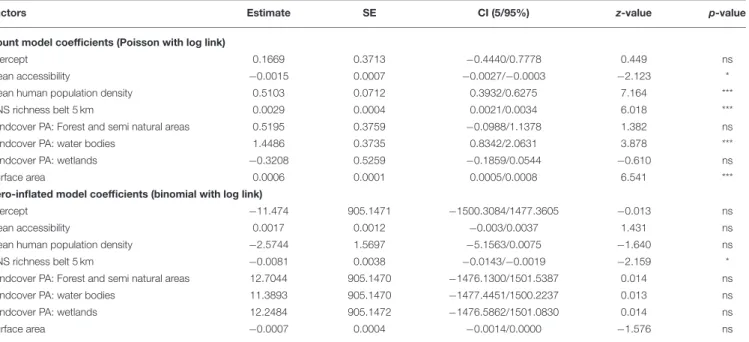
The results of the Zero-Inflated Negative Binomial regression show a significant positive relationship between NNS richness in PAs and richness in the associated 5-km belts (Table 1,
Figure 4). NNS richness in the 5-km belts was also the only significant variable in the zero part of the model (i.e., modeling PAs free of NNS), being lower when surrounding PAs with no recorded NNS.
The most abundant land cover in the majority of PAs was “Forest and semi natural areas” (525 PAs, 78.6%) followed by “Wetlands” (99 PAs, 14.8%) and “Waterbodies” (42 PAs, 6.3%) (Figure 4). Agricultural area was the most abundant land cover of only two PAs. The count part of the ZINB model shows that the number of NNS in PAs was highest where water bodies were the most abundant land cover (Table 1). The number of NNS in PAs also significantly increased with increasing mean human population density in the PAs and the surface area of PAs, and was negatively correlated with travel time to large cities (Table 1,
Figure 4).
Temporal Sequence
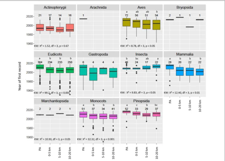
Year of First Records in PAs and Associated Belts Overall, NNS were recorded later in PAs than in any of the three associated belts, with the difference on average being 4.5 years (0–5 km), 6 years (5–10 km), and 5.5 years (10– 20 km) (Figure 5). The average years of first records in the three belts were not significantly different. Of the NNS present in both the PA and the associated 5-km belt, 59.4% were recorded earlier in the belt, 17.5% in the same year and 23.1% earlier in the PAs. This overall pattern of delayed records in the PAs was observed for 5 of the 11 taxonomic classes (Figure 6). Of the top 9 NNS in PAs, six were recorded significantly earlier in the PAs than in at least one of the belts (Kruskal-Wallis-Test: X² = 62.21, df = 3, p < 0.001) (Supplementary Figure 2).
DISCUSSION
Our study provides an extensive nationwide analysis of how the NNS community in the vicinity of PAs influences the NNS community inside PAs. Using data on 1,602 non-native terrestrial
FIGURE 3 | The nine most frequent NNS in PAs (left) and 5-km belts (right). Ecological impact classification assessed by the Norwegian Biodiversity Information Centre (NBIC, https://www.biodiversity.no) shown inside the bar: SE, “Severe Impact;” PH, “Potentially High Impact;” and LO, “Low Impact;” on ecology. (Credit pictures: B. canadensis & N. vison: T.M. Blackburn; A. pseudoplatanus: Willow, CC BY-SA 2.5; S. racemosa: Opioła Jerzy, CC BY 2.5; P. stichensis: Rosser1954, CC BY-SA 4.0; S. fontinalis: marrabbio2, CC BY-SA 3.0; E. canadensis: Christian Fischer, CC BY-SA 3.0; L. sauveolens: AfroBrazilian, CC BY-SA 3.0; L. polyphyllus: Andreas Eichler, CC BY-SA 4.0; R. rugosa: Vihljun, public domain; R. japonica: Andrea Moro, CC BY-SA 4.0; B. vulagris: Stefan.lefnaer, CC BY-SA 4.0; N. caerulescens: Konrad Lackerbeck, CC BY-SA 2.5).
TABLE 1 | Results from the Zero-Inflated Negative Binomial regression model (ZINB) between non-native species (NNS) richness in protected areas (PAs) and mean accessibility to PAs, mean human population density in the PAs, NNS richness in 5-km belts, land cover type (Agriculture, Forest and semi natural areas, Water bodies, Wetlands) in the PAs and surface area of the PAs.
Factors Estimate SE CI (5/95%) z-value p-value
Count model coefficients (Poisson with log link)
Intercept 0.1669 0.3713 −0.4440/0.7778 0.449 ns
Mean accessibility −0.0015 0.0007 −0.0027/−0.0003 −2.123 * Mean human population density 0.5103 0.0712 0.3932/0.6275 7.164 *** NNS richness belt 5 km 0.0029 0.0004 0.0021/0.0034 6.018 *** Landcover PA: Forest and semi natural areas 0.5195 0.3759 −0.0988/1.1378 1.382 ns Landcover PA: water bodies 1.4486 0.3735 0.8342/2.0631 3.878 *** Landcover PA: wetlands −0.3208 0.5259 −0.1859/0.0544 −0.610 ns Surface area 0.0006 0.0001 0.0005/0.0008 6.541 *** Zero-inflated model coefficients (binomial with log link)
Intercept −11.474 905.1471 −1500.3084/1477.3605 −0.013 ns Mean accessibility 0.0017 0.0012 −0.003/0.0037 1.431 ns Mean human population density −2.5744 1.5697 −5.1563/0.0075 −1.640 ns NNS richness belt 5 km −0.0081 0.0038 −0.0143/−0.0019 −2.159 * Landcover PA: Forest and semi natural areas 12.7044 905.1470 −1476.1300/1501.5387 0.014 ns Landcover PA: water bodies 11.3893 905.1470 −1477.4451/1500.2237 0.013 ns Landcover PA: wetlands 12.2484 905.1472 −1476.5862/1501.0830 0.014 ns Surface area −0.0007 0.0004 −0.0014/0.0000 −1.576 ns
Log-likelihood: −736.8 on 16 DF. 671 PAs were considered.
***significant at p < 0.001; *significant at p < 0.05; ns: not significant.
and freshwater animals and plants of Norway, we showed that 77% of the PAs included in our analysis were free from any of them. This result is in accordance with a previous study on a global scale, which found more than 90% of PAs free from
any of 894 non-native animals (Liu et al., 2020). The absence of NNS in PAs is often attributed to their remoteness, which keeps them far from areas where many NNS are introduced: the introduction of NNS is often associated with trading and
FIGURE 4 | Response of Non-native species (NNS) richness in protected areas (PAs) to: (A) NNS richness in 5 km-belts, (B) Mean human population density in the PAs, (C) Mean accessibility of PAs, (D) Most abundant land cover in the PA (AG, Agricultural areas; FSNA, Forest and semi natural areas; WB, Water bodies; WL, Wetlands) and (E) Surface area of the PA. Solid blue line and shaded area represent the mean and standard error of NNS richness, fitted by GAM.
transport activities between cities and countries (Banks et al., 2015; Nunes et al., 2015; Seebens et al., 2017b; Seebens, 2019) and NNS further spread by vectors such as roads, streams or intended and unintended human transportation (Leuven et al., 2009; Nunes et al., 2015; Brancatelli and Zalba, 2018; Ward et al., 2020). However, in our study, the low NNS richness in the 5-km belts surrounding PAs was the only variable explaining variation in the presence or absence of NNS in PAs (i.e., the zero part of the ZINB regression). This suggests that low colonization and propagule pressure in close proximity seems to be a better explanatory factor for the absence of NNS in PAs than their accessibility. For PAs occupied by NNS, their NNS richness was again significantly related to NNS richness in the surrounding 5-km belts, the accessibility of PAs having a lower effect (i.e., the count part of the ZINB regression). These results again support our hypothesis of a quantitative effect of the pool of NNS in areas close to PAs on the richness of NNS within the PAs. Nevertheless, three other factors also influenced the richness of NNS in PAs: their surface area, the human population density inside them and the main type of habitat they contain. PAs in which water bodies were the most abundant habitat had the highest NNS richness, highlighting lakes and rivers as corridors for the colonization of both limnic (Leuven et al., 2009) and terrestrial NNS (Malíková and Prach, 2010; Francis et al., 2019).
The temporal analysis carried out in our study revealed that NNS were recorded earlier in the immediate surroundings of PAs than within them. On average, NNS were recorded in the PAs 4.5 years after being recorded in the 0–5 km belts. We also measured a delay in the first records of NNS in the PAs for
FIGURE 5 | Year of first records in protected areas and their associated belts 0–5, 5–10, and 10–20 km for the 196 non-native species recorded within protected areas. We selected only non-native species present in protected areas. For each non-native species, we compared protected areas and their associated belts. The numbers above the boxes represent the numbers of first records of the non-native species included in the analysis. Small letters (a, b) indicate elements that are significantly different from each other according to a Dunn’s test for pairwise comparison following a significant Kruskal-Wallis Test (KW).
five of the eleven taxonomic classes of NNS and six of the nine most frequent NNS found in PAs. This spatio-temporal sequence of occurrence confirms that PAs are not prime locations for
FIGURE 6 | Boxplot NNS species taxonomic classes present in PAs: The year of first record in PAs and within a distance of 0–5, 5–10, and 10–20 km from the PA (associated belts). The numbers above the boxes represent the numbers of first records of the non-native species. Small letters (a, b, c) indicate elements that are significantly different from each other according to Dunn’s test with “fdr” adjustment, following a significant Kruskal-Wallis Test (KW).
the introduction of NNS and further suggests the important role of colonizing events from within a few kilometers of their boundaries in the processes involved in the spread of NNS in PAs. These results also suggest an invasion debt, i.e., the time lag between the introduction of a non-native species into a region and its potentially negative ecological consequences (Rouget et al., 2016). For example, ornamental plants already introduced for horticultural purposes, but not yet naturalized (i.e., not yet established as persistent wild populations outside of cultivation), represent a risk of invasion in the future that could be exacerbated by climate change (Haeuser et al., 2018). Once naturalized, the time it takes for an invasive species to reach remote PAs, potentially containing many threatened native species, may be another element of this debt. Garden lupin (L. polyphyllus), for example, considered a severely impacting NNS, which was most common in the 0–5 km belts, but much less common in PAs, should require special consideration in their management. This pattern is also supported by the
qualitative similarity that we observed within and around PAs, with, on average, two thirds of the NNS present in a specific PA also present in its associated 5-km belt. Nonetheless, previous studies have shown that successful colonization of new environments by NNS varies from species to species depending on environmental conditions and species characteristics (Sakai, 2001; Gallien and Carboni, 2017). Differences in environmental conditions inside and outside PAs, as already shown by Mas (2005), could explain differences in species frequency inside and around PAs. For instance, the Garden lupin (L. polyphyllus) the most frequent NNS in the 5-km belts, is an ornamental plant which is common in Norwegian gardens from where it escaped from cultivation (Fermstad, 2010). Another example of differences in environmental conditions are reflected by the fact that the proportions of NNS of two classes, Aves and Pinopsida, were higher inside PAs than in their surroundings. Ten of the 12 non-native birds were Anseriformes (ducks, geese and swans), thus dependent on aquatic habitats, such as
the Canada goose (B. canadensis), which is the most frequent NNS in the PAs. The Canada goose utilizes open and grassy habitats and nearby lakes and other water bodies, feeding on aquatic plants and animals amongst other food (Jansson et al., 2008). Concerning the conifers (class of Pinopsida), suitable habitats comprise forest and semi natural areas, which was the most abundant land cover type in the majority of the PAs in our study. Non-native waterfowl and conifers may thus find more suitable habitat in PAs than around them, as many PAs, unlike belts, have probably been delineated to include high conservation value habitats such as water bodies and forests.
Our analyses show that invasive NNS (i.e., listed on the Norwegian, 2012 blacklist) are over-represented in Norwegian PAs compared to non-invasives. Invasive NNS accounted for 12% of the NNS in the 5-km belts but 40% in the PAs. Furthermore, 57% of invasive NNS present in 5-km belts are also present inside PAs. This high colonization success of invasive NNS in PAs may be explained by their high abundance outside PAs and by having characteristics that permit their fast colonization and spread. In the belt, an invasive NNS was, on average, four times as abundant as a non-invasive NNS (with species abundance measured as the number of records). Several studies have already demonstrated the crucial role of propagule pressure, and especially the number of new immigrants, on the colonization success of NNS (Cassey et al., 2018; Alzate et al., 2020). The higher abundance of invasive NNS in the belts could thus result in a higher propagule pressure inside PAs, and a subsequent higher probability of establishment of invasive NNS in PAs. Four NNS - R. rugosa, R. japonica, N. caerulescens and B. vulgaris – were all among the top 9 NNS in 5-km belts but not among the top 9 NNS in PAs. These are clear candidates for future colonization of PAs. This information is of relevance for managers of PAs to remain vigilant to future non-native colonizers.
In conclusion, our study strongly emphasizes the role of colonizing events from the surroundings of PAs in shaping NNS communities inside PAs. Both the abundance and the composition of the NNS communities around PAs influence NNS within PAs. Moreover, our study also reveals differences which are highly relevant for the conservation of PAs, such as the over-representation of invasive NNS within PAs. For all these reasons, we strongly suggest expanding the focus of NNS management within PAs to beyond PA boundaries as recommended by
Monaco and Genovesi (2014). Considering the significance of the impact of invasive NNS in PAs (Hulme et al., 2014), efforts in monitoring and controlling invasive NNS are required from the PA management authorities, but also surrounding landowners. Similar advice has already been provided for PAs surrounded by high human population densities (Spear et al., 2013; Liu et al., 2020) - our study generalizes and reinforces it. The focus on NNS in the vicinity of PAs is of relevance for future conservation strategies, especially to prevent incursions of NNS with severe ecological impacts.
DATA AVAILABILITY STATEMENT
Publicly available datasets were analyzed in this study. This data can be found at: https://artskart.artsdatabanken.no and https:// www.protectedplanet.net.
AUTHOR CONTRIBUTIONS
KH did the analysis. KH and AC wrote the first draft of the manuscript. All authors commented, approved the manuscript, and conceived the study.
FUNDING
KH has received funding from the European Union’s Horizon 2020 research and innovation programme under the Marie Skłodowska-Curie grant agreement No. 766417.
ACKNOWLEDGMENTS
We thank the editors of Frontiers in Ecology and Evolution for this Special Issue. Further, we would like to thank two reviewers for their supportive and constructive comments on the manuscript. We also thank the Norwegian Biodiversity Information Centre (NBIC) for providing their database on alien species. The opinions given herein belong solely to the authors and do not represent the views or policies of IUCN.
SUPPLEMENTARY MATERIAL
The Supplementary Material for this article can be found online at: https://www.frontiersin.org/articles/10.3389/fevo. 2020.625137/full#supplementary-material
List Data Providers:
Agder naturmuseum ARC, Arkeologisk Museum UiS, BioFokus, Ecofact, Ento Consulting, Faun Naturforvaltning AS, GBIF-noder utenfor Norge, JBJordal, MFU, MiljÃ,direktoratet, MiljÃ,lÃ|re.no, Molltax, Multiconsult, Naturhistorisk Museum – UiO, Naturrestaurering AS, Norges miljÃ,- og biovitenskapelige universitet, botanisk forening, Norsk entomologisk forening, Norsk institutt for naturforskning, Norsk institutt for vannforskning, Norsk Ornitologisk Forening, Norsk zoologisk forening, NTNU-Vitenskapsmuseet, RÃUdgivende Biologer AS, Svalbardflora.net, Sweco Norge AS, TromsÃ, museum – Universitetsmuseet, Universitetsmuseet i Bergen, UiB.
Supplementary Figure 1 | Spearman rank correlation index of non-native species (NNS) richness in protected areas (PAs) and the four continuous explanatory variables: Mean accessibility of PAs, surface area of PAs, NNS richness in 5-km belts and mean human population density in PAs. Supplementary Figure 2 | Years of first record of NNS in PAs and within a distance of 0–5, 5–10, and 10–20 km from the PA (belt zones). The numbers above the boxplot indicate the numbers of PAs and associated belts in which the NNS were present. Small letters (a,b) indicate elements that are significantly differentiated from each other according to Dunn’s Test with “fdr” adjustment following a significant Kruskal-Wallis Test (KW).
REFERENCES
Achim, Z., Kleiber, C., and Jackman, S. (2008). Regression models for count data in R. J. Stat. Softw. 27, 1–25. doi: 10.18637/jss.v027.i08
Alzate, A., Onstein, R. E., Etienne, R. S., and Bonte, D. (2020). The role of preadaptation, propagule pressure and competition in the colonization of new habitats. Oikos 129, 820–829. doi: 10.1111/oik.06871
Banks, N. C., Paini, D. R., Bayliss, K. L., and Hodda, M. (2015). The role of global trade and transport network topology in the human-mediated dispersal of alien species. Ecol. Lett. 18, 188–199. doi: 10.1111/ele.12397
Bellard, C., Cassey, P., and Blackburn, T. M. (2016). Alien species as a driver of recent extinctions. Biol. Lett. 12:20150623. doi: 10.1098/rsbl.2015.0623 Blackburn, T. M., Bellard, C., and Ricciardi, A. (2019). Alien versus native
species as drivers of recent extinctions. Front. Ecol. Environ. 12:20150623. doi: 10.1002/fee.2020
Brancatelli, G. I. E., and Zalba, S. M. (2018). Vector analysis: a tool for preventing the introduction of invasive alien species into protected areas. Nat. Conserv. 24, 43–63. doi: 10.3897/natureconservation.24.20607
Cassey, P., Delean, S., Lockwood, J. L., Sadowski, J. S., and Blackburn, T. M. (2018). Dissecting the null model for biological invasions: a meta-analysis of the propagule pressure effect. PLoS Biol. 16:e2005987. doi: 10.1371/journal.pbio.2005987
CBD (2020). Convention on Biological Diversity. Available online at: https://www. cbd.int/ (accessed September 2, 2020).
Chapman, D., Purse, B. V., Roy, H. E., and Bullock, J. M. (2017). Global trade networks determine the distribution of invasive non-native species. Glob. Ecol. Biogeogr. 26, 907–917. doi: 10.1111/geb.12599
Clavero, M., and García-Berthou, E. (2005). Invasive species are a leading cause of animal extinctions. Trends Ecol. Evol. 20:110. doi: 10.1016/j.tree.2005.01.003 CLC (2018). © European Union, Copernicus Land Monitoring Service 2018.
European Environment Agency (EEA), Available online at: https://land. copernicus.eu
de Pooter, M., Pagad, S., and Ullah, I. (2007). Invasive Alien Species and Protected Areas-A Scoping Report Part I. Available online at: http://www.issg. org (accessed October 20, 2020).
Dimitrakopoulos, P. G., Koukoulas, S., Galanidis, A., Delipetrou, P., Gounaridis, D., Touloumi, K., et al. (2017). Factors shaping alien plant species richness spatial patterns across Natura 2000 special areas of conservation of Greece. Sci. Total Environ. 601–602, 461–468. doi: 10.1016/j.scitotenv.2017.05.220 Fermstad, E. (2010). NOBANIS-Invasive Alien Species Fact Sheet- Lupinus
Polyphyllus. From: Online Database of European Network on Invasive Alien Species-NOBANIS www.nobanis.org.
Foxcroft, L. C., Jarošík, V., Pyšek, P., Richardson, D. M., and Rouget, M. (2011). Protected-area boundaries as filters of plant invasions. Conserv. Biol. 25, 400–405. doi: 10.1111/j.1523-1739.2010.01617.x
Francis, R. A., Chadwick, M. A., and Turbelin, A. J. (2019). An overview of non-native species invasions in urban river corridors. River Res. Appl. 35, 1269–1278. doi: 10.1002/rra.3513
Gallardo, B., Aldridge, D. C., González-Moreno, P., Pergl, J., Pizarro, M., Pyšek, P., et al. (2017). Protected areas offer refuge from invasive species spreading under climate change. Glob. Chang. Biol. 23, 5331–5343. doi: 10.1111/gcb.13798 Gallien, L., and Carboni, M. (2017). The community ecology of invasive species:
where are we and what’s next? Ecography 40, 335–352. doi: 10.1111/ecog.02446 Haeuser, E., Dawson, W., Thuiller, W., Dullinger, S., Block, S., Bossdorf, O., et al. (2018). European ornamental garden flora as an invasion debt under climate change. J. Appl. Ecol. 55, 2386–2395. doi: 10.1111/1365-2664.13197
Hettinger, N. (2001). Defining and evaluating exotic species: issues for yellowstone park policy. Western N Am. Nat. 61, 257–260.
Hortal, J., Lobo, J. M., and Jiménez-Valverde, A. (2007). Limitations of biodiversity databases: case study on seed-plant diversity in Tenerife, Canary Islands. Conserv. Biol. 21, 853–863. doi: 10.1111/j.1523-1739.2007.00686.x
Hulme, P. E., Pyšek, P., Pergl, J., Jarošík, V., Schaffner, U., and Vilà, M. (2014). Greater focus needed on alien plant impacts in protected areas. Conserv. Lett. 7, 459–466. doi: 10.1111/conl.12061
Intergovernmental science-policy platform on biodiversity and ecosystem services, I (2019). Summary for Policymakers of the Global Assessment Report on Biodiversity and Ecosystem Services (Paris: Zenodo).
IUCN (2016). IUCN. Available online at: https://www.iucn.org/theme/species/our-work/invasive-species (accessed September 2, 2020).
Jackman, S. (2020). pscl: Classes and Methods for R Developed in the Political Science Computational Laboratory. United States Studies Centre, University of Sydney. Sydney, NSW. Available online at: https://github.com/atahk/pscl/ (acessed October 20, 2020).
Jansson, K., Josefsson, M., and Weidma, I. (2008). NOBANIS – Invasive Alien Species Fact Sheet –Branta canadensis. From: Online Database of the North European and Baltic Network on Invasive Alien Species – NOBANIS www. nobanis.org.
Jari´c, I., and Cvijanovi´c, G. (2012). The tens rule in invasion biology: measure of a true impact or our lack of knowledge and understanding? Environ. Manage 50, 979–981. doi: 10.1007/s00267-012-9951-1
Kortz, A. R., and Magurran, A. E. (2019). Increases in local richness (α-diversity) following invasion are offset by biotic homogenization in a biodiversity hotspot. Biol. Lett. 15:20190133. doi: 10.1098/rsbl.2019.0133
Lambdon, P. W., Lloret, F., and Hulme, P. E. (2008). Do non-native species invasions lead to biotic homogenization at small scales? The similarity and functional diversity of habitats compared for alien and native components of Mediterranean floras. Divers. Distribut. 14, 774–785. doi: 10.1111/j.1472-4642.2008.00490.x
Lawal, B. H. (2012). Zero-inflated count regression models with applications to some examples. Qual. Quant. 46, 19–38. doi: 10.1007/s11135-010-9324-x Leuven, R. S. E. W., Velde, G., van der Baijens, I., Snijders, J., Zwart,
C., van der Lenders, H. J. R., et al. (2009). The river Rhine: a global highway for dispersal of aquatic invasive species. Biol. Invasions 11:1989. doi: 10.1007/s10530-009-9491-7
Liu, X., Blackburn, T. M., Song, T., Wang, X., Huang, C., and Li, Y. (2020). Animal invaders threaten protected areas worldwide. Nat. Commun. 11:2892. doi: 10.1038/s41467-020-16719-2
Malíková, L., and Prach, K. (2010). Spread of alien Impatiens glandulifera along rivers invaded at different times. Ecohydrol. Hydrobiol. 10, 81–85. doi: 10.2478/v10104-009-0050-8
Mas, J.-F. (2005). Assessing protected area effectiveness using surrounding (buffer) areas environmentally similar to the target area. Environ. Monit. Assess 105, 69–80. doi: 10.1007/s10661-005-3156-5
Mathur, V. B., Onial, M., and Mauvais, G. (2015). “Managing threats,” in Protected Area Governance and Management, eds G. L. Worboys, M. Lockwood, A. Kothari, S. Feary, and I. Pulsford (Canberra, NSW: ANU Press), 473–494. Available online at: https://www.jstor.org/stable/j.ctt1657v5d. 23 (accessed September 3, 2020).
McKinney, M. L., and Lockwood, J. L. (1999). Biotic homogenization: a few winners replacing many losers in the next mass extinction. Trends Ecol. Evol. 14, 450–453. doi: 10.1016/S0169-5347(99)01679-1
McNeely, J. A., Mooney, H. A., Neville, L. E., Schei, P. J., and Waage, J. K. (2001). Global Strategy on Invasive Alien Species. Available online at: https://portals. iucn.org/library/node/7882 (accessed September 8, 2020).
Meiners, S., and Pickett, S. T. A. (2013). “Plant invasion in protected landscapes: exception or expectation?,” in Plant Invasions in Protected Areas: Patterns, Problems and Challenges. eds L. C. Foxcroft, D. M. Richardson, and P. Pyšek, et al. (Dordrecht: Springer). doi: 10.1007/978-94-007-7750-7_3
Monaco, A., and Genovesi, P. (2014). European Guidelines on Protected Areas and Invasive Alien Species. Available online at: https://portals.iucn.org/library/sites/ library/files/documents/2014-070.pdf (accessed March 15, 2017).
Moustakas, A., Voutsela, A., and Katsanevakis, S. (2018). Sampling alien species inside and outside protected areas: does it matter? Sci. Total Environ. 625, 194–198. doi: 10.1016/j.scitotenv.2017.12.198
Nelson, A. (2008). Travel Time to Major Cities: A Global Map of Accessibility. Available online at: https://forobs.jrc.ec.europa.eu (accessed July 25, 2019). Nunes, A., Tricarico, E., Panov, V., Cardoso, A., and Katsanevakis, S. (2015).
Pathways and gateways of freshwater invasions in Europe. Aquatic Invasions 10, 359–370. doi: 10.3391/ai.2015.10.4.01
R Core Team (2019). R: A Language and Environment for Statistical Computing. R Foundation for Statistical Computing (Vienna).
Ramakrishnan, A. P., Musial, T., and Cruzan, M. B. (2010). Shifting dispersal modes at an expanding species’ range margin. Mol. Ecol. 19, 1134–1146. doi: 10.1111/j.1365-294X.2010.04543.x
Rodrigues, A. S. L., Akçakaya, H. R., Andelman, S. J., Bakarr, M. I., Boitani, L., Brooks, T. M., et al. (2004). Global gap analysis: priority regions for expanding the global protected-area network. Bioscience 54, 1092–1100. doi: 10.1641/ 0006-3568(2004)054[1092:GGAPRF]2.0.CO;2
Rouget, M., Robertson, M. P., Wilson, J. R. U., Hui, C., Essl, F., Renteria, J. L., et al. (2016). Invasion debt – quantifying future biological invasions. Divers. Distrib. 22, 445–456. doi: 10.1111/ddi.12408
Sakai, A. K. (2001). The population biology of invasive species. Annu. Rev. Ecol. Syst. 32, 305–332. doi: 10.1146/annurev.ecolsys.32.081501.114037
Sandvik, H., Hilmo, O., Finstad, A. G., Hegre, H., Moen, T. L., Rafoss, T., et al. (2019). Generic ecological impact assessment of alien species (GEIAA): the third generation of assessments in Norway. Biol. Invasions 21, 2803–2810. doi: 10.1007/s10530-019-02033-6
Seebens, H. (2019). Invasion ecology: expanding trade and the dispersal of alien species. Curr. Biol. 29, R120–R122. doi: 10.1016/j.cub.2018.12.047
Seebens, H., Blackburn, T. M., Dyer, E. E., Genovesi, P., Hulme, P. E., Jeschke, J. M., et al. (2017a). No saturation in the accumulation of alien species worldwide. Nat. Commun. 8:14435. doi: 10.1038/ncomms14435
Seebens, H., Blackburn, T. M., Dyer, E. E., Genovesi, P., Hulme, P. E., Jeschke, J. M., et al. (2018). Global rise in emerging alien species results from increased accessibility of new source pools. PNAS 115, E2264–E2273. doi: 10.1073/pnas.1719429115
Seebens, H., Essl, F., and Blasius, B. (2017b). The intermediate distance hypothesis of biological invasions. Ecol. Lett. 20, 158–165. doi: 10.1111/ele. 12715
Spear, D., Foxcroft, L. C., Bezuidenhout, H., and McGeoch, M. A. (2013). Human population density explains alien species richness in protected areas. Biol. Conserv. 159, 137–147. doi: 10.1016/j.biocon.2012.11.022
Troudet, J., Grandcolas, P., Blin, A., Vignes-Lebbe, R., and Legendre, F. (2017). Taxonomic bias in biodiversity data and societal preferences. Sci. Rep. 7:9132. doi: 10.1038/s41598-017-09084-6
Tsiamis, K., Gervasini, E., Deriu, I., D’amico, F., Katsanevakis, S., and de Jesus Cardoso, A. (2019). Baseline Distribution of Species Listed in the 1st Update of Invasive Alien Species of Union Concern. Luxembourg: EUR 29675 EN,
Publications Office of the European Union,. Available online at: https://data. europa.eu/doi/10.2760/75328 (accessed December 4, 2020).
Ward, S. F., Taylor, B. S., Dixon Hamil, K.-A., Riitters, K. H., and Fei, S. (2020). Effects of terrestrial transport corridors and associated landscape context on invasion by forest plants. Biol. Invasions 22, 3051–3066. doi: 10.1007/s10530-020-02308-3
WDPA, UNEP-WCMC and IUCN (2019). Protected Planet: Norway: The World Database on Protected Areas (WDPA)/OECM. Cambridge: UNEP-WCMC and IUCN. Available online at: http://protectedplanet.net.
Worboys, G. L. (2015). “Concept, purpose and challenges,” in Protected Area Governance and Management, eds G. L. Worboys, M. Lockwood, A. Kothari, S. Feary, and I. Pulsford (Canberra, NSW: ANU Press), 9–42.
WorldPop (2018). (www.worldpop.org - School of Geography and Environmental Science, University of Southampton; Department of Geography and Geosciences, University of Louisville; Departement de Geographie, Universite de Namur) and Center for International Earth Science Information Network (CIESIN), Columbia University Global High Resolution Population Denominators Project - Funded by The Bill and Melinda Gates Foundation (OPP1134076).
Conflict of Interest:The authors declare that the research was conducted in the absence of any commercial or financial relationships that could be construed as a potential conflict of interest.
The handling editor declared a past co-authorship with one of the authors, TB. Copyright © 2021 Holenstein, Simonson, Smith, Blackburn and Charpentier. This is an open-access article distributed under the terms of the Creative Commons Attribution License (CC BY). The use, distribution or reproduction in other forums is permitted, provided the original author(s) and the copyright owner(s) are credited and that the original publication in this journal is cited, in accordance with accepted academic practice. No use, distribution or reproduction is permitted which does not comply with these terms.