HAL Id: hal-02976450
https://hal.archives-ouvertes.fr/hal-02976450
Submitted on 23 Oct 2020
HAL is a multi-disciplinary open access
archive for the deposit and dissemination of
sci-entific research documents, whether they are
pub-lished or not. The documents may come from
teaching and research institutions in France or
abroad, or from public or private research centers.
L’archive ouverte pluridisciplinaire HAL, est
destinée au dépôt et à la diffusion de documents
scientifiques de niveau recherche, publiés ou non,
émanant des établissements d’enseignement et de
recherche français ou étrangers, des laboratoires
publics ou privés.
A new spectroscopic method for measuring the
temperature gradient in the solar photosphere
M. Faurobert, S. Criscuoli, M. Carbillet, G. Contursi
To cite this version:
M. Faurobert, S. Criscuoli, M. Carbillet, G. Contursi. A new spectroscopic method for measuring the
temperature gradient in the solar photosphere: Generalized application in magnetized regions.
Astron-omy and Astrophysics - A&A, EDP Sciences, 2020, 642, pp.A186. �10.1051/0004-6361/202037736�.
�hal-02976450�
A&A 642, A186 (2020) https://doi.org/10.1051/0004-6361/202037736 c M. Faurobert et al. 2020
Astronomy
&
Astrophysics
A new spectroscopic method for measuring the temperature
gradient in the solar photosphere
Generalized application in magnetized regions
M. Faurobert
1, S. Criscuoli
2, M. Carbillet
1, and G. Contursi
11 Université Côte d’Azur, Observatoire de la Côte d’Azur, CNRS UMR 7293 J.L. Lagrange Laboratory, Campus Valrose,
06108 Nice, France
e-mail: [email protected], [email protected]
2 National Solar Observatory, Boulder, CO, USA
e-mail: [email protected]
Received 14 February 2020/ Accepted 21 July 2020
ABSTRACT
Context.The contribution of quiet-Sun regions to the solar irradiance variability is currently unclear. Certain solar-cycle variations of the quiet-Sun’s physical structure, such as the temperature gradient, might affect the irradiance. Accurate measurements of this quantity over the course of the activity cycle would improve our understanding of long-term irradiance variations.
Aims.In a previous work, we introduced and successfully tested a new spectroscopic method for measuring the photospheric tempera-ture gradient directly on a geometric scale in the case of non-magnetic regions. In this paper, we generalize this method for moderately magnetized regions that may be encountered in the quiet solar photosphere.
Methods. To simulate spectroscopic observations, we used synthetic Stokes profiles I and V of the magnetic FeI 630.15 nm line and intensity profiles of the non-magnetic FeI 709 nm line computed from realistic three-dimensional magneto-hydrodynamical sim-ulations of the photospheric granulation and line radiative transfer under local thermodynamical equilibrium conditions. We then obtained maps at different levels in the line-wings by convolution with the instrumental point spread function (PSF) under var-ious conditions of atmospheric turbulence – with and without correction by an adaptive optics (AO) system. The PSF were ob-tained with the PAOLA software and the AO performance is inspired by the system that will be operating on the Daniel K. Inouye Solar Telescope.
Results. We considered different conditions of atmospheric turbulence and photospheric regions with different mean magnetic strengths of 100 G and 200 G. As in non-magnetic cases studied in our previous work, the image correction by the AO system is mandatory for obtaining accurate measurements of the temperature gradient. We show that the non-magnetic line at 709 nm may be safely used in all the cases we have investigated. However, the intensity profile of the magnetic-sensitive line is broadened by the Zeeman effect, which would bias our temperature-gradient measurement. We thus implemented a correction procedure of the line profile for this magnetic broadening in the case of weakly magnetized regions. In doing so, we remarked that in the weak-field regime, the right- and left-hand (I+ V and I − V) components have similar shapes, however, they are shifted in opposite directions due to the Zeeman effect. We thus reconstructed the intensity profile by shifting back the I + V and I − V profiles and by adding the re-centered profiles. The measurement then proceeds as in the non-magnetic case. We find that this correction procedure is efficient in regions where the mean magnetic strength is smaller or on the order of 100 G.
Conclusions.The new method we implement here may be used to measure the temperature gradient in the quiet Sun from ground-based telescopes equipped with an efficient AO system. We stress that we derive the gradient on a geometrical scale and not on an optical-depth scale as we would do with other standard methods. This allows us to avoid any confusion due to the effect of temperature variations on the continuum opacity in the solar photosphere.
Key words. techniques: high angular resolution – techniques: spectroscopic – Sun: photosphere
1. Introduction
The variation of the total solar irradiance (TSI) in phase with the solar cycle has been well-established thus far thanks to mea-surements performed in space by dedicated instruments over the past four solar cycles. However, long-term variations of the TSI at solar minimum are still under debate because different groups that have used different composite data have either found a constant or a varying TSI at solar minimum (see the reviews byYeo et al. 2014;Solanki et al. 2013). Moreover, the spectral dependance (SSI) of the solar cycle variability is also a con-troversial topic (e.g.,Ermolli et al. 2013). These variations are
an important forcing term for the evolution of the climate on Earth (e.g., Lean 2017). In recent years, solar irradiance vari-ability studies have also been motivated by the necessity for achieving an understanding of and modeling stellar variability (Fabbian et al. 2017;Faurobert 2019) which, in turn, may ham-per exoplanet detectability (e.g., Cegla 2019) and affect both
the determination of the physical properties of exoplanet atmo-spheres (e.g.,Kowalski et al. 2019) and the abundance of bio-markers (e.g.,Grenfell 2017).
The efforts made to model TSI and SSI variations cur-rently rely on the hypothesis that the main drivers of solar variability are magnetic features at the solar surface and that
Open Access article,published by EDP Sciences, under the terms of the Creative Commons Attribution License (https://creativecommons.org/licenses/by/4.0), which permits unrestricted use, distribution, and reproduction in any medium, provided the original work is properly cited.
the thermodynamical state of the quiet-Sun atmosphere is invariant. Other plausible mechanisms that imply a modula-tion of the global structure of the Sun have also been pro-posed. Ideas on global structural changes are supported by the observation of the frequencies of the acoustic p-modes that also show a well-documented solar-cycle variation (see
Fossat et al. 1987; Salabert et al. 2015). Possible contributions of the quiet Sun to long-term variations of the irradiance could be investigated via a systematic long-term follow-up of the photospheric temperature gradient. Intensity center-to-limb vari-ation in continua and lines is a well-known tool for estimat-ing the physical properties of stellar atmospheres, in particular, the temperature gradient. Nevertheless, several studies have indicated that the shape of the intensity limb darkening in photospheric continua remains constant with time and, in par-ticular, no variation has been reported with the magnetic activity cycle (e.g., Petro et al. 1984; Elste & Gilliam 2007). Recently,
Criscuoli & Foukal (2017) employed three-dimensional (3D) magneto-hydrodynamic (MHD) simulations of the solar pho-tosphere to show that variations of the temperature gradient that are consistent with cyclic variations of unresolved magnetic fields produce variations of the intensity limb darkening shape that are below the precision of modern instrumentation.
More sensitive measurement methods are needed to attain progress in that field. In Faurobert et al. (2018; Paper I), we therefore tested a new spectroscopic method that allows us to measure the photospheric temperature gradient. One of the main advantages of this method is that it yields the temperature gradient on a geometric scale without having to rely on atmo-spheric models. With standard methods based on the measure-ment of center-to-limb variation in continua, we can obtain the temperature gradient on an optical-depth scale. Yet, as the con-tinuous absorption coefficient is highly dependent on tempera-ture, a variation of the temperature gradient induces variations of the optical depth scale in such a way that the temperature at the formation depth of the continuum varies very little. In other words, even if the temperature gradient would vary on a geometrical scale, its variations on the continuum optical-depth scale would be very small and the center-to-limb variation of the continuum intensity would be hardly detectable. This effect is described in greater detail in Faurobert et al. (2016) and it may bring on some insights with regard to the negative results ofCriscuoli & Foukal(2017). This is why the method we have developed is based on a completely different approach. We use a very sensitive differential-interferometry technics to measure the perspective shift between images formed in the continuum and in the wing of a spectral line when they are observed away from disk center. This allows us to measure the formation-depth difference between the images directly on a geometrical scale. In Paper I, the tests were performed on synthetic data derived from 3D-hydrodynamical simulations of the photosphere. However, the photosphere of the quiet Sun is not magnetic-free. The quiet Sun magnetism has been investigated for decades and it contin-ues to stand as a challenging qcontin-uestion. A thorough review of the subject is presented in Bellot Rubio & Orozco Suárez (2019). The most sophisticated inversion method, namely, the spatially-coupled inversion applied to Hinode/SOT spectropolarimetric observations, allows for the inference of the probability distribu-tion funcdistribu-tion of the magnetic strength in inter-network regions. Its average value was found to be on the order of 130 G at optical depth unity (Danilovic et al. 2016).
Here, we present a generalization of our method that is aimed at dealing with magnetized regions of the quiet Sun. We used snapshots from the same time series of 3D-MHD
simulations that were employed inCriscuoli & Foukal(2017) to investigate the constancy of the center-to-limb variations of pho-tospheric continua. Specifically, we employed snapshots from the Copenhagen-Stagger code (Galsgaard & Nordlund 1996), which are representative of quiet and modest activity regions. We computed the simulated data by performing radiative trans-fer calculations of both the intensity and circular polarization in the FeI 630.15 nm line that was used in Paper I. In addition to this magnetic line, we also computed the intensity profiles of the non-magnetic line of FeI at 709 nm.
As in Paper I, we wish to study the feasibility of ground-based measurements under different conditions of turbulence in the Earth atmosphere. The image degradation at a telescope focus due to atmospheric turbulence is related to the so-called Fried parameter r0, which represents the coherence scale of the
turbulent motions. Here, we used four values for r0, r0= 15 cm,
12 cm, 7 cm, and 5 cm. The value of 7 cm is the median value measured at the Haleakala site where the National Science Foun-dation’s Daniel K. Inouye Solar Telescope (DKIST) is located. The point spread functions (PSFs) in the different situations are obtained from the PAOLA software (Jolissaint 2006,2010) and for the characteristics of the adaptive optics (AO), we refer to the description of the system that will operate on DKIST, which was presented inJohnson et al.(2016) andMarino et al.(2016)
In Sect.2, we explain the procedure we introduced to correct the line profile for the Zeeman broadening of the FeI 630.15 nm line and we recall very briefly the main steps of the measurement method that was presented in more detail in the previous papers, namely,Faurobert et al.(2018,2016). Section3is devoted to the presentation of the results.
2. Measurement method and synthetic data
2.1. Synthetic data
We used 3D radiative MHD simulations of the solar pho-tosphere produced with the Copenhagen-Stagger code, which is a dedicated magneto-hydrodynamics code that solves the time-dependent equations for conservation of mass, momen-tum, and energy together with the induction equation. For our analysis, we employed a total of ten snapshots, obtained from simulation runs initialized with a vertical unipolar mag-netic field of '100 G and '200 G, respectively, which were then evolved until a statistically stationary state was reached. We note that in this state, the magnetic field is concen-trated by advection into intergranular lanes and at the ver-tices of granules, where it forms sheet-like and micropore-like structures, while the average magnetic field remains close to the initial one (Fabbian et al. 2012;Fabbian & Moreno-Insertis 2015). Each snapshot covers an area of 6 × 6 Mm2 on the solar surface with a horizontal spatial sampling of 24 km pixel−1. Snapshots from these simulation runs have already been employed in a variety of studies (e.g., Fabbian et al. 2012;Beck et al. 2013;Criscuoli 2013;Criscuoli & Uitenbroek 2014a,b;Fabbian & Moreno-Insertis 2015), including an inves-tigation of the cyclic variation of the intensity center-to-limb variation of solar photospheric continuum mentioned in Sect.1
(Criscuoli & Foukal 2017). We refer to Fabbian et al. (2010,
2012) and Fabbian & Moreno-Insertis (2015) for a detailed description of the simulations. Stokes I and V emerging from the simulated photospheres were synthezised with the Rybicky and Hummer code (RH,Uitenbroek 2001) at different inclination angles. The syntheses were performed assuming Local Thermo-dynamic Equilibrium at the spectral ranges of the 630.1 nm and A186, page 2 of10
M. Faurobert et al.: Temperature gradient in the low solar photosphere
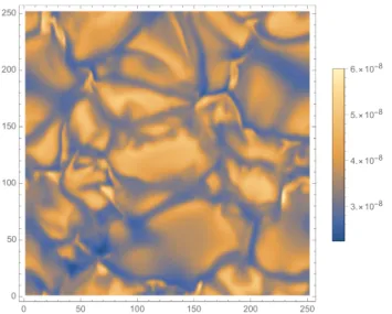
3.× 10-8 4.× 10-8 5.× 10-8 6.× 10-8
Fig. 1.Synthetic image of the granulation in the 630 nm continuum at cos θ= 0.9. The pixel size is 0.032600
.
709.0 nm FeI lines. The atomic parameters employed for the syn-theses were derived from the Kurucz database1, adjusted so that the average spectra emerging along the vertical direction from a set of ten purely hydrodynamic snapshots, also obtained with the Stagger code, matched the observed ones. We note that zero micro-turbulence was assumed and the non-thermal Doppler broadening of spectral lines only uses the self-consistent velocity fields taken directly from the three-dimensional simulations.
For a given inclination angle (location on the solar disk), we obtain cubes of simulated I(x, y, λ) and V(x, y, λ) data that repre-sent solar scenes. We show in Fig.1a continuum image obtained at the heliocentric angle θ with cos θ = 0.9 for one snapshot of the MHD simulation. In Fig. 2, we show the magnetic-flux map computed with the center-of-gravity method (Semel 1970;
Uitenbroek 2003) applied to the FeI 630.15 nm line. The mean value of the unsigned longitudinal magnetic component at this disk position is 75 G. We observe the concentration of the mag-netic field in the inter-granular lanes, where it may reach val-ues up to 1 kG. Figure3shows the histogram of the longitudinal magnetic component at the formation depth of the line-wings for this snapshot of the simulation. Most of the pixels have longitu-dinal magnetic fields smaller than 250 G.
To obtain synthetic cubes of (x, y, λ) data observed with a telescope, we need to convolve the solar scene with the PSF of the instrument that accounts for the image degradation due to tur-bulence in the Earth atmosphere (with or without AO correction) and the diffraction by the telescope pupil and by the spectrograph slit. For the diffraction, we assume that the telescope has a 4 m diameter off-axis mirror like the DKIST and the spectrograph profile is a Gaussian function with a half-width of 2.1 pm. In the absence of atmospheric turbulence, the spatial resolution due to the diffraction by the telescope mirror is λ/D = 0.032500 at
630 nm, which is very close to the resolution of the numerical simulation and the line profiles are only slightly broadened. To compute the convolution of the images with the PSF, we over-sampled the simulated images by a linear interpolation between the grid points to get a pixel size of 0.0132500 that is slightly smaller than the Shannon criteria for both the 630.15 nm and the 709 nm lines. Then we re-binned the images to a pixel size of 0.05300× 0.10600 to account for a typical observing mode with
a spectrograph slit-width of 0.10600 that would be used for this
1 Available athttp://kurucz.harvard.edu/ -50 0 50 100 150 200 250
Fig. 2.Synthetic magnetic-flux map for a snapshot of the simulation initialized with a vertical field of 100 G.
-50 0 50 100 150 200 250 0 5000 10 000 15 000 20 000 25 000
Fig. 3.Histogram of the values (in Gauss) of the longitudinal compo-nent of the magnetic field in the same snapshot of the MHD simulation as in Fig.2.
observing program. As found in Paper I, photon noise and read-out noise are negligible for a typical exposure time of 0.5 s.
To model the PSF of the system (atmosphere+telescope+AO system), we made use of the semi-analytical code PAOLA (Jolissaint 2006,2010) as described in Paper I, for four values of the Fried parameter, namely r0= 5, 7, 12, 15 cm,
correspond-ing respectively to bad, median, good, and excellent seecorrespond-ing at the Aleakala site. Two cases of long-exposure post-AO PSFs (bad seeing case and excellent seeing case), together with the corresponding seeing-limited PSFs and the ideal PSF (no per-turbation at all) are presented in Fig.4. We should note that the corresponding Strehl ratios range from 0.125 (bad seeing case) to 0.727 (excellent seeing case). The full-width at half-maximum (FWHM) is, in turn, greatly enhanced, basically changing from ∼rλ
0 to ∼ λ
D, where D denotes the diameter of the telescope. The
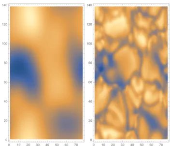
simulated PSFs were then used for convolution with the vari-ous previvari-ously modeled solar scenes in order to obtain the final observed images (assuming stability of the correction on the whole field of observation). The resulting images in the con-tinuum are shown in Fig. 5 (excellent seeing case) and Fig.6
(bad seeing case). It is worthwhile to note that the contrasts in these images greatly benefit from the AO correction. The con-trast, thus, goes from 0.019 to 0.066 in the bad seeing case (with a gain of ∼3.5) and from 0.065 to 0.129 in the excellent seeing case (with a gain of ∼2.0).
Fig. 4.Logarithmic plot of the simulated post-AO and seeing-limited PSFs for the cases of excellent seeing (r0 = 15) and bad seeing (r0 =
5 cm) compared with the ideal PSF.
Fig. 5. Left panel: continuum image obtained without AO for atmo-spheric turbulence, r0 = 15 cm, for one snapshot of the granulation at
µ = 0.9. Right panel: continuum image with AO for the same r0value.
The pixel size is 0.05300
along the slit direction (y-axis) and 0.10600
in the x-direction.
2.2. From spectrograms to images at constant continuum optical depth
To measure the mean temperature gradient, we must measure the mean temperature on constant continuum optical-depth surfaces. So, we have to construct images formed on surfaces at a roughly constant continuum optical-depth spanning a depth range from the deepest visible layers around continuum optical-depth unity to the highest accessible altitudes. Our reconstruction method relies on the relation between the line and continuum absorption coefficients in the Lorentzian damping wings of a line.
2.2.1. In the absence of a magnetic field
In the absence of a magnetic field, or for non-magnetic lines, the line opacity that varies steeply with the wavelength is given by
k(λ)= kc+ klφ((λ − λ0)/∆λD), (1)
where kcis the continuum opacity, klis the frequency-averaged
line opacity, λ0 is the line center wavelength in the observer
frame, and φ is the normalized absorption profile (which in
Fig. 6.Same as Fig.5for r0= 5 cm.
the general case is given by the Voigt function), and ∆λD is
the line Doppler width. In the following, we use the notations δλ = (λ − λ0)/∆λD and r = kl/kc. The Doppler broadening
is due both to thermal broadening and to unresolved velocities. The ratio of line to continuum absorption coefficients is equal to 1+ rφ(δλ). The absorption profile and r vary over the solar surface because of temperature, velocity, density, while the line central wavelength varies as a result of the varying global con-vective motions of the matter with respect to the observer. The line central wavelength is defined as the position of the minimum of the line-intensity profile.
For a given value of the line cord λ − λ0, the ratios of line to
continuum absorption show significant variations over the solar surface because of the Doppler-width and line-strength varia-tions. So, to recover images at a constant continuum optical depth, we use the line information in a non-standard way, which we explain in the following.
First, we show that at small line depressions the shape of the intensity profile follows the shape of the absorption profile rφ. For a line formed under local thermodynamical equilibrium, the radiative transfer equation along a given line of sight is written as dI(λ, τc) dτc = 1+ kl kc φ(δλ) ! (I(λ, τc) − B(τc)), (2)
where we use the continuum optical depth τcas the depth
vari-able and B denotes the Planck function.
As in Milne-Eddington models, we now assume that the ratios r= kl/kcand φ are depth-independent and that the Planck
function is a linear function of the continuum optical depth, B(τc)= B0+ B1τc. The emergent intensity is then given by
I(λ)= B0+ B1− B1
rφ(δλ)
1+ rφ(δλ)· (3)
The emergent intensity in the continuum (where rφ(δλ) = 0) is Ic= B0+ B1and the line depression at wavelength λ is
Ic− I(λ)= B1
rφ(δλ)
1+ rφ(δλ)· (4)
In the far wings of the line, rφ(δλ) 1, so the line depression is proportional to the line absorption profile. Furthermore, the A186, page 4 of10
M. Faurobert et al.: Temperature gradient in the low solar photosphere Voigt function decreases as a/[√π(δλ)2], where a denotes the
Voigt parameter (seeMihalas 1978, p. 281). We take advantage of this property to construct maps of the line intensity at a con-stant value of rφ(δλ) over the solar surface.
To do so, we first consider at each pixel of the solar scene the line-cord width at 2% line depression, denoted by ∆λcand
we define line-cord levels at given fractions of ∆λc, namely
∆λi = αi∆λc, with αi < 1. In the line damping-wings, we have
rφ(δλi) ' (1/α2i)rφ(δλc). The ratio of line to continuous
absorp-tion is thus constant over a map of intensity at constant α. To obtain a fine enough depth grid, we chose to consider 25 line cords given by∆λi= (i − 1)∆λc/24. For the FeI 630.15 nm line,
the damping wings correspond to levels 15 to 25; whereas for the weaker 709 nm line, they correspond to levels between 20 and 25. This approach, which relies on Eq. (4), is valid when r and the line-absorption profile are depth-independent or do not vary significantly within the line-wing formation height. In AppendixA, we present a test of this image reconstruction method in the wings of the FeI 630.15 nm line.
2.2.2. In the presence of a weak magnetic field
Next, we consider the case where the line has a Landé factor different from zero and is formed in a region of the quiet Sun where weak inhomogeneous magnetic fields are present. This situation is likely to appear in the inter-network. In that case, the magnetic fields affect the line absorption profile because of the Zeeman splitting of the atomic levels. When the Zeeman splitting is smaller than the Doppler broadening, the Zeeman effect acts as an additional broadening mechanism. The line also gets polarized and the line radiation field may be described by a four-component vector with the four Stokes parameters (I, Q, U, V). The polarized radiative transfer equation becomes a vectorial equation where the 4 × 4-absorption matrix couples the Stokes parameters. However, in the case of weak Zeeman effect one can show that, at first order, the linear polarization described by the two parameters Q and U is negligible and that it is possible to derive two decoupled radiative transfer equations for the two quantities I + V and I − V, that is, the intensities of the left- and right-hand circular polarization sig-nals in the line (see Sánchez Almeida & Trujillo Bueno 1999;
Landi Degl’Innocenti & Landolfi 2004, p. 404). These equations are formally identical to the scalar equation that holds for non-polarized radiation, namely,
d(I ± V)
ds = −(kI± kV)(I ± V)+ jL± jV, (5)
where s denotes the position along the line of sight, kI is the
usual line absorption coefficient, kV is the absorption coefficient
for Stokes V, and jI and jV are emissivity terms. In the weak
Zeeman-effect regime, kV kI and jV jI. The
absorp-tion coefficients for the two signals I ± V are slightly shifted in wavelength in opposite directions with respect to the absorption coefficient kI. The value of the shift depends on the magnetic
component along the line of sight. This gives rise to an additional magnetic broadening of the line intensity profile I, obtained as the half-sum of the two signals.
In order to apply the image construction method recalled above, we need to correct the line profile for this magnetic broad-ening. To do so, we shift the I+ V and I − V profiles to put them on a same arbitrary wavelength position before adding them. We recover an intensity profile that is just the sum of the left- and right-hand circular profiles. Its Lorentzian wings are not modi-fied by the magnetic field.
-15 -10 -5 0 5 0 5000 10 000 15 000 20 000
Fig. 7.Histogram of the displacement (in mÅ) between the left-hand and right-hand circular polarization in the FeI 630.15 nm line in a snap-shot of the MHD simulation initialized with a vertical field of 100 G, where the average unsigned longitudinal magnetic field is 75 G.
In the following, we show that this correction method gives good results for the measurements performed with the FeI 630.15 nm line when the averaged magnetic flux over the area is smaller or on the order of 100 G. For larger values, the weak Zeeman regime is not valid anymore.
In effect, the weak field regime is valid for magnetic field strength, verifying the condition gB 2500 G for a typical iron line formed in the solar photosphere (see
Landi Degl’Innocenti & Landolfi 2004, p. 397). Thus, for the FeI 630.15 nm line, g= 1.67, so the weak field regime is extended to B 1500 G. We show in Fig.3the histogram of the vertical component of the magnetic field in a snapshot of the MHD simulation initialized with a vertical magnetic field of 100 G, where the mean unsigned longitudinal magnetic component is 75 G. We also show in Fig. 7 the histogram of the Zeeman shift between the left-hand and right-hand circular polarization profiles and we verify that it is, indeed, in a large fraction of the pixels, much smaller than the Doppler width of the line that is on the order of 30 mÅ. Here, we note that the differential interferometry technics that we implemented to measure the formation-depth difference between images relies on the cross-spectrum of the images. This Fourier method requires the use of full compact images so that we cannot eliminate any pixel in the images. This is the reason why we need to perform tests to assess its validity in the case where the weak field regime does not take hold everywhere throughout the observed region.
2.3. Temperature measurement
Assuming that the FeI 630.15 nm and the 709 nm lines are formed under local thermodynamical equilibrium (LTE) condi-tions in the solar photosphere, we may derive the mean tem-perature from the intensity in the images at the different line levels. The LTE assumption has been tested by various authors (seeShchukina & Trujillo Bueno 2001) and, in Paper I, we also tested it for the FeI 630.15 nm line through a comparison with the Hinode SOT/SP observations.
In Paper I, we computed the mean temperature at a given line level from the mean intensity in the image and we compared its depth-variation to a semi-empirical model of the quiet photo-sphere. Here, we proceed differently as we wish to test the tem-perature measurement with respect to the temtem-perature-gradient derived from the MHD simulation itself. So, we compute the A186, page 5 of10
temperature by inverting the Planck law at each pixel of the image and we average the temperature maps for every line level. 2.4. Measurement of the formation-depth
We first measure the depth difference between the formation height of the line-cord images and the continuum level. This is achieved exactly in the same way as described in Paper I (see alsoFaurobert et al. 2016), that is, we measure the perspective shift along the radial direction between images taken in a line wing and in the continuum when they are observed away from disk center, that is, at heliocentric angles different from 0. We stress that the depth-difference is obtained in km or in second of arc, without any reference to a model.
To measure this very small displacement, we use the phase of the cross-spectrum of the continuum and line-wing images. This Fourier method requires us to consider the power spectra of intensity fluctuations in images taken rigorously at the same time in the continuum and in the line. In effect, we have to observe the same granular structures at both levels, but only slightly shifted by the perspective effect. This is why we need spectroscopic observations, however 2D images are not needed as far as the spectrograph slit is oriented radially, namely, in the direction of the perspective shift. In practice, we use 1D power spectra of the intensity variations along the spectrograph slit and we sum over all the slit positions to decrease the statistical noise on the cross-spectrum. Denoting Ii(x) and Ic the 1D cuts of the
line-wing and continuum images, respectively, and assuming that the line-wing image is similar to the continuum one, but slightly dis-placed radially at a distance, δ, by the perspective effect, we can write
Ii(x) ∼ Ic(x − δ) (6)
and
bIi(u) ∼ bIc(u) exp(2iπuδ). (7)
Shifts can then be derived from the phase of the cross-spectrum. We used a series of spectrograms to estimate the cross-spectrum
b
Qcibetween Ic(x) and Ii(x):
b
Qci(u)= hbIc(u)bIi∗(u)i
∼ h| bIc(u) |2ie−2iπδu, (8)
where bI∗
i(u) represents the conjugate Fourier transform of Ii(x),
and the brackets refer to the ensemble average. A linear fit of the phase variation with respect to the spatial frequency variable, u, allows us to measure δ. We stress here that this method allows us to measure very small displacements between images, as it is not limited by the spatial resolution of the instrument. The main limitation is the signal-to-noise ratio (S/N) of the granu-lation spectrum and the domain of validity of Eq. (6), that is, based on the assumption of similarity between the line-wing and continuum images.
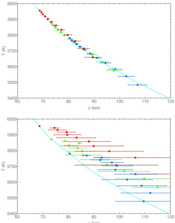
Still, we can only measure differences between image-formations heights. We need to know where our reference image in the continuum is formed. Here, we simply compute the mean temperature in the continuum image and assume that it obeys the temperature-law derived from the simulation. This means that the reference point in our (T, z) plots at each heliocentric angle is always, by construction, on the curve derived from the simula-tion. We stress again here that we can only measure temperature gradients. 60 70 80 90 100 110 120 5400 5500 5600 5700 5800 5900 6000 z km T K 60 70 80 90 100 110 120 5400 5500 5600 5700 5800 5900 6000 z km T K
Fig. 8.Temperature gradient measured on five snapshots of the simula-tion with hBi ' 100 G using the FeI 630.15 nm line under bad seeing conditions (r0 = 5 cm). The light-blue full line shows the
tempera-ture gradient derived from the simulation. Red dots: measurements at µ = 0.9, green dots: measurements at µ = 0.8, blue dots: measurements at µ= 0.7. The error bars show the one-sigma uncertainty on the depth measurements. Upper panel: with AO, lower panel: without AO.
3. Results
The measurements of temperatures and depth-differences between the images were performed by averaging over five snap-shots of the MHD simulation and for three positions on the solar disk at µ= 0.9, 0.8, 0.7. We considered the images at levels 14 to 25 for the strong FeI 630.15 nm line and at levels 19 to 25 for the weaker FeI 709 nm one. We recall that our method is meant to be applied to images obtained in the Lorentzian damping wings of a line. Figure8shows the comparison between the temperature gradient derived from the simulation with hBi ' 100 G and the results of the measurements on the images in the FeI 630.15 nm line, in the case of a bad seeing with r0= 5 cm without and with
AO correction. Figure9 shows the same comparison for mea-surements performed on images in the FeI 709 nm. We see that for both lines, the AO correction is crucial for obtaining mean-ingful measurements.
As in Paper I, measurements performed on perturbed images are biased and show large error bars. However, by implementing the AO correction and the correction for the Zeeman broadening presented above, we can accurately measure the temperature gra-dient from images in the magnetic-sensitive line. The measure-ments are even more accurate when one uses the non-magnetic line but, as the line is weaker, it gives access to lower altitudes. We also notice that more images can be used in the strong line that has stronger damping wings. This allows us to check the consistency of the measurements because the depth intervals A186, page 6 of10
M. Faurobert et al.: Temperature gradient in the low solar photosphere 60 70 80 90 100 5600 5700 5800 5900 6000 z km T K 60 70 80 90 100 5600 5700 5800 5900 6000 z km T K
Fig. 9. Same as Fig. 8, but for measurements performed in the FeI 709 nm line.
spanned at different heliocentric angles are partially superim-posed so we may get several measurements at the same depth from different heliocentric positions. For example, we notice in Fig.8that the measurement performed at µ= 0.9 allows to reach altitudes between 70 km and 90 km (red dots in the figure) and that the measurements are consistent with the ones that are per-formed at µ= 0.8 (green dots) and µ = 0.7 (blue dots). We also notice that the error bars become larger for measurements per-formed on images at smaller line levels; the reason for this is that at smaller line levels, in other words, closer to the line core, there is a change of regime of the absorption profile from Lorentz to Doppler and the assumption of similarity between the continuum and line-wing images (Eq. (6)) cannot be verified fully.
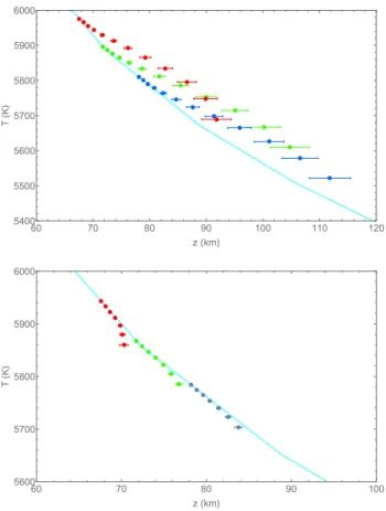
Figure10shows the results obtained from both lines in the case of the MHD simulation initialized with a vertical mag-netic field of 200 G. We assumed median seeing conditions (r0 = 7 cm) with AO correction. We clearly see that using the
magnetic-sensitive line leads to a temperature gradient that is too low and also leads to inconsistent measurements at differ-ent heliocdiffer-entric angles. The non-magnetic line may still be used but we remark that the measurements performed on images at level 19, that is, those forming at higher altitudes, deviate signif-icantly from the expected values. This effect is probably related to stronger depth-variations of the physical parameters affecting the line formation in the presence of stronger magnetic fields. We recall that the method we are testing here relies on the assump-tion that the images in the continuum are similar to the images in the line wings but shifted radially by the perspective effect.
The comparison between the two lines clearly points out that the Zeeman-broadening correction we have implemented is not valid in the case where hBi ' 200 G. This method is based on the approximation of weak Zeeman effect so it is not surprising that
60 70 80 90 100 110 120 5400 5500 5600 5700 5800 5900 6000 z km T K 60 70 80 90 100 5600 5700 5800 5900 6000 z km T K
Fig. 10.Temperature gradient measured on five snapshots of the sim-ulation with hBi ' 200 G with AO under median seeing conditions (r0 = 7 cm). Color code applied as above. Upper panel: obtained with
the FeI 630.15 nm line, lower panel: obtained with the non-magnetic line FeI 709 nm.
it fails above a certain magnetic-strength limit. Our tests show that this limit is between 100 G and 200 G.
4. Conclusion
In this paper, we test a method for measuring the tempera-ture gradient in the low solar photosphere of the quiet Sun from a ground-based instrument with AO correction. In a pre-vious work, we investigated the non-magnetic case using radia-tive hydrodynamical simulations of the granulation from the S
tagger
-code. As the quiet solar photosphere is likely to be permeated with mixed-polarity magnetic fields on the order of 100 G, the method has to be tested with simulations where mag-netic fields are taken into account. To do so, we used snapshots from the MURaM code initialized with uniform vertical mag-netic fields of 100 G and 200 G and we performed polarized 3D radiative transfer calculations to derive simulated intensity and circular polarization profiles in the FeI 630.15 nm magnetic line and intensity profiles in the non-magnetic 709 nm line. Then the observed solar scenes at different line-cord levels were derived through a convolving with the PSF of the telescope and atmo-spheric turbulence with and without adaptive optics.The method for measuring the temperature gradient from the images is similar to what we presented in Paper I, the dif-ference being that we had to correct the intensity profiles in the FeI 630.15 nm line for the Zeeman effect. In the presence of mixed-polarity magnetic fields on the order of 100 G, the Zeeman effect acts as an additional broadening mechanism. We A186, page 7 of10
proposed a correction procedure based on the weak Zeeman effect approximation where the left- and right- hand circular-polarization components are simply shifted symmetrically with respect to the line center in the absence of magnetic field.
Our results show that AO corrections is necessary to obtain-ing a satisfyobtain-ing measurement of the temperature gradient. We also show that implementing the Zeeman-broadening correction allows us to safely use the magnetic FeI 630.15 nm line to derive the temperature gradient in magnetic regions up to mean mag-netic strengths of 100 G, but that it fails when hBi ' 200 G. The weak Zeeman-effect approximation breaks down for mag-netic strength between those two values. In that case, the mea-surements made with the non-magnetic line are still relevant, but they span a smaller altitude range.
Acknowledgements. This work was supported by a grant of the University côte d’Azur and by the DKIST project. The DKIST is managed by the National Solar Observatory (NSO), which is operated by the Association of Universities for Research in Astronomy, Inc. (AURA) under a cooperative agreement with the National Science Foundation (NSF). The snapshots of magneto- convection simulations were provided to us by Elena Khomenko and were calculated by F. Moreno Insertis and D. Fabbian using the computing resources of the Mare Nostrum (BSC/CNS, Spain) and DEISA/HLRS (Germany) super- computer installations.
References
Beck, C., Fabbian, D., Moreno-Insertis, F., Puschmann, K. G., & Rezaei, R. 2013,A&A, 557, A109
Bellot Rubio, L., & Orozco Suárez, D. 2019,Liv. Rev. Sol. Phys., 16, 1
Cegla, H. 2019,Geosciences, 9, 114
Criscuoli, S. 2013,ApJ, 778, 27
Criscuoli, S., & Foukal, P. 2017,ApJ, 835, 99
Criscuoli, S., & Uitenbroek, H. 2014a,ApJ, 788, 151
Criscuoli, S., & Uitenbroek, H. 2014b,A&A, 562, L1
Danilovic, S., van Noort, M., & Rempel, M. 2016,A&A, 593, A93
Elste, G., & Gilliam, L. 2007,Sol. Phys., 240, 9
Ermolli, I., Matthes, K., Dudok de Wit, T., et al. 2013,Atmos. Chem. Phys., 13, 3945
Fabbian, D., & Moreno-Insertis, F. 2015,ApJ, 802, 96
Fabbian, D., Khomenko, E., Moreno-Insertis, F., & Nordlund, Å. 2010,ApJ, 724, 1536
Fabbian, D., Moreno-Insertis, F., Khomenko, E., & Nordlund, Å. 2012,A&A, 548, A35
Fabbian, D., Simoniello, R., Collet, R., et al. 2017,Astron. Nachr., 338, 753
Faurobert, M. 2019, inChapter 8 – Solar and Stellar Variability, eds. O. Engvold, J. C. Vial, & A. Skumanich, 267
Faurobert, M., Balasubramanian, R., & Ricort, G. 2016,A&A, 595, A71
Faurobert, M., Carbillet, M., Marquis, L., Chiavassa, A., & Ricort, G. 2018,
A&A, 616, A133
Fossat, E., Gelly, B., Grec, G., & Pomerantz, M. 1987,A&A, 177, L47
Galsgaard, K., & Nordlund, Å. 1996,J. Geophys. Res., 101, 13445
Grenfell, J. L. 2017,Phys. Rep., 713, 1
Johnson, L. C., Cummings, K., Drobilek, M., et al. 2016, inAdaptive Optics
Systems V, Proc. SPIE, 9909, 99090Y
Jolissaint, L. 2006,PASP, 118, 1205
Jolissaint, L. 2010,J. Eur. Opt. Soc., 5, 10055
Kowalski, A., Schrijver, K., Pillet, V., & Criscuoli, S. 2019,BAAS, 51, 149
Landi Degl’Innocenti, E., & Landolfi, M. 2004,Polarization in Spectral Lines
(Dordrecht: Kluwer Academic Publisher), 307
Lean, J. 2017,Oxford Research Encuclopedia(Oxford: Oxford University Press) Marino, J., Carlisle, E., & Schmidt, D. 2016, inAdaptive Optics Systems V,
Proc. SPIE, 9909, 99097C
Mihalas, D. 1978,Stellar Atmospheres(San Francisco: W.H. Freeman) Petro, L. D., Foukal, P. V., Rosen, W. A., Kurucz, R. L., & Pierce, A. K. 1984,
ApJ, 283, 426
Salabert, D., García, R. A., & Turck-Chièze, S. 2015,A&A, 578, A137
Sánchez Almeida, J., & Trujillo Bueno, J. 1999,ApJ, 526, 1013
Semel, M. 1970,A&A, 5, 330
Shchukina, N., & Trujillo Bueno, J. 2001,ApJ, 550, 970
Solanki, S. K., Krivova, N. A., & Haigh, J. D. 2013,ARA&A, 51, 311
Uitenbroek, H. 2001,ApJ, 557, 389
Uitenbroek, H. 2003,ApJ, 592, 1225
Yeo, K. L., Krivova, N. A., & Solanki, S. K. 2014,Space Sci. Rev., 186, 137
M. Faurobert et al.: Temperature gradient in the low solar photosphere
Appendix A: Mean intensity in reconstructed line-wing images
In this appendix, we present a test of the method we use to relate the mean intensity in line-wing images to the mean tempera-ture at constant continuum optical depth surfaces. This method is based on a Milne-Eddington model of the line formation. We start by explainining the testing procedure. It uses both observa-tions of the intensity profile in the line wings and a realistic 3D numerical simulation of the line formation. The test is then car-ried out on the FeI 630.15 nm line using observations obtained onboard the Hinode satellite and a numerical simulation from the Stagger code.
A.1. Test procedure
We start from the expression of the line depression given in Eq. (4). In the far wings of the line, where rφ(δλ) 1, the line depression is proportional to the line absorption profile and we can write
rφ(δλi)=
Ic− I(∆λi)
B1
, (A.1)
where we consider the line intensity at the line cords ∆λi =
(i − 1)∆λc/24 that have been introduced in Sect.2.2.1. We recall
that Icand I denote respectively the continuum intensity and the
line-wing intensity at a given location on the solar surface. We obtain an average value of rφ(δλi) from Eq. (A.1) by
replac-ing the line depression by its average over the image and B1
by an average value extracted from a realistic numerical simu-lation of the photospheric granusimu-lation. From this expression of rφ(δλi), we derive an estimate of the average formation depth
of the emergent line-wings intensity at the line cords∆λiwhich,
according to the Milne-Eddington model, is given by τf(∆λi)=
cos θ 1+ rφ(δλi)
(A.2) for observations performed at the heliocentric angle θ. Then we compare this estimate of the formation depth to the continuum optical-depth where the average Planck function of the 3D sim-ulation is equal to the observed average intensity at the line-cord ∆λi. If both values agree, we conclude that our averaging method
is consistent and that the line-wing images at the line cords∆λi
may be used to recover the average temperature on constant con-tinuum optical-depth surfaces.
A.2. Test on Hinode observations in the FeI 630.15 nm profile We perform the test described above on observations of the FeI 630.15 nm line obtained onboard the Hinode satellite with the SOT/SP instrument. We use center-to-limb observations taken on 19 December 2007 in the quiet Sun and we record the line intensity at the 25 line-cords defined in the text, then we average it on surfaces of 2000× 2000 at µ = cos θ = 0.9, 0.8,
0.7. The line depression observed at levels 15 to 25 is shown in Fig. A.1 for these three values of µ. To calibrate the num-ber of counts in Hinode data in physical units the mean signal measured in the continuum at the center of the solar disk was identify to the mean continuum intensity at µ = 1 derived from the 3D-numerical simulation.
We also use the numerical simulation to estimate B1. To do
so, we extract from the simulation the values of the Planck func-tion on constant continuum optical-depth surfaces and we then
16 18 20 22 24 5.0× 10¹² 1.0× 10¹³ 1.5× 10¹³ 2.0× 10¹³ 2.5× 10¹³ 3.0× 10¹³ Line-cord level Ic (μ )-I( δλ ,μ )
Fig. A.1.Line depression, in cgs units, at the line-cord levels 15 to 25 averaged over 2000
× 2000
images, for three values of µ. Blue line: µ = 0.7, green line: µ= 0.8, orange line: µ = 0.9.
0.4 0.5 0.6 0.7 0.8 0.9 1.0 1.1 2.0× 10¹⁴ 2.2× 10¹⁴ 2.4× 10¹⁴ 2.6× 10¹⁴ 2.8× 10¹⁴ 3.0× 10¹⁴ 3.2× 10¹⁴ τc B ( τc )
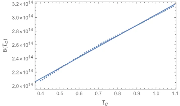
Fig. A.2.Dotted line: mean value of the Planck function on constant τc
surfaces. Full line: linear fit.
0.5 0.6 0.7 0.8 0.9 1.0 0.5 0.6 0.7 0.8 0.9 1.0 τc τf
Fig. A.3.Vertical axis: formation-depth of the average line-wing radi-ation according to the Milne-Eddington model; horizontal axis: contin-uum optical depth where the average Planck function is equal to the average line-wing radiation. Red dots are line cords 15 to 25 at µ= 0.9; green dots are line cords 15 to 25 at µ= 0.8, blue dots are line cords 15 to 25 at µ= 0.7. Dashed lines show the first bisector.
compute their average as a function of τc. We obtain the result
shown in Fig.A.2, where we also show the linear fit that allows us to derive B1.
We can now obtain the values of rφ(δλi) at the line cords
15 to 25 by using Eq. (A.1) and the Milne-Eddington formation depths τf(δλ) given by Eq. (A.2). We then compare these
for-mation depths to the continuum optical depths where the Planck A186, page 9 of10
function is equal to the observed emergent intensity at the same line cord. The comparison is shown in Fig.A.3. Both values are in good agreement for the line-cords 15 to 25 at the three values of µ.
The test, hence, is positive and shows that the Milne-Eddington model does quite a good job in capturing the main physical ingredients of the line-wing formation when spatially-averaged profiles are concerned. We also point out that the
relation between the formation depth and the line depression is valid only in the line-wings. Furthermore, we stress that the spa-tial averaging of the line profile is done at line cords∆λi, which
vary from pixel to pixel over the solar surface, following the vari-ation of the Doppler width in the granular structures. Averaging at constant line-cords would not be userful because the relevant wavelength variable is the distance from the central wavelength of the line measured in Doppler-width units.

![[PDF] Cours PowerPoint 2007 pour débutant en pdf | Cours informatique](data:image/gif;base64,R0lGODlhAQABAIAAAP///wAAACH5BAEAAAAALAAAAAABAAEAAAICRAEAOw==)