Discrete Representations of n-Dimensional Wave Equations
and Their Applications to Quantum Mechanics
by
Hrvoje J. Hrgovci6
Submitted to the Department of Physics
in Partial Fulfillment of the Requirements for the Degree of Doctor of Philosophy
at the
Massachusetts Institute of Technology July, 1992
@1992 Hrvoje J. Hrgovi6 All rights reserved.
The author hereby grants to M.I.T. permission to reproduce and to distribute copies of this thesis document in whole or in part.
Signature of Author
Certified by
Accepted by
Department of Physics
July 5, 1992
Dr. Tommaso Toffoli, Thesis Supervisor
Dr. George Koster, Chairman, Physics Department Committee on Graduate Students
MASSACHUSETTS INSTITUTE, OF TFCHNO.OGY
Abstract
A simple model of many-body quantum mechanics governed by completely local in-teractions in ordinary three-dimensional space is presented. The equations of motion, involving no Euclideanization of time, are elementary extensions of those describing random walks on a square lattice, and are far simpler than those obtained through standard path-integral theory. A quantity is defined in terms of populations of par-ticles on the lattice, whose expectation value is proportional to the square of the multi-particle wave functions associated with the system; for sufficiently microscopic measurement scales, this generalized 'density' may take on negative values, thereby circumventing the constraints imposed by Bell's inequality.
1
Introduction
The general solution of the one-dimensional wave equation may be written as a sum of two functions, or traveling waves. The equations of motion of these traveling waves, first-order in time and space, are simple translations in opposite directions with a constant speed.
Section 2 of this paper extends the benefits of such an approach to higher dimen-sions, so that in general, the n-dimensional wave equation is likewise recast as a sum of 2n functions, first order in time, each of which is associated with motion along the positive or negative directions of the n axes of the space. The domain of the wave functions is a discrete space-time lattice; nevertheless, the resultant wave equations and their solutions display relativistic covariance in the continuum limit.
Section 3 shows that this traveling wave decomposition lends itself to a statis-tical implementation. Recall that the kernel of the diffusion equation is expressible as the continuum limit of distributions of random walks on a lattice, and that the time evolution of the diffusion equation may be computed by ensembles of particles executing such random walks. By assigning these particles a (discrete) phase factor, it is possible to give the wave equation a similar implementation, one that is much simpler than those obtained by way of standard path integral theory.
Section 4 shows that this statistical rendering of the wave equation can be used to construct a model of multi-particle quantum mechanics, in an ordinary three-di-mensional configuration space, in a Minkowski metric. In general, a single particle state (or collection thereof) is represented, or simulated, by a gas-like distribution of particles propagating throughout the lattice at once. A large ensemble of such distributions may then be used to obtain the correct quantum mechanical probabilities associated with both single and multi-particle states. This is because there exists a quantity, additive in the number of these ensemble members, whose expectation value is likewise equal to the square of the corresponding wave functions.
mechanical aspects of this formalism to macroscopic phenomena. The final section discusses related formalisms, and compares them to the present one. The appendices show how the traveling wave decomposition may be applied to the scalar Klein-Gordon equation, the Dirac equation, and Maxwell's equations in a Lolentz gauge. Each of these cases are straightforward generalizations of the scalar equations, whereby the topology of the lattice and the coefficients of the associated transition matrices are altered in direct correspondence to the internal structure of the associated particles. The mass, and also the potentials, are then introduced as perturbations induced by Poissonly distributed random fields, bypassing the more complicated formalism of Higgs particles. The appendix also considers some mathematical properties of the associated scalar wave solutions.
2 The Discrete Wave Equation
The discrete analogue of the wave equation is defined on an orthonormal, (n + 1)-dimensional space-time lattice of points whose spacing is unity. The second order partial derivatives of time and space appearing in the D'Alembertian are replaced by their usual finite-difference analogues
02
where...)
i + 1,.) - 2(...,xi,+
(...,-
1,)
where
Xi = X l,X, 2 ..., Xn, t
Thus, the wave equation retains its usual form,
1c
0t2 = d2 2- + '+ .( 2)9 (2)+ +
Setting the constant c, which will be called the speed of light, to 1/n confers several useful properties on the equations, among them, a conserved momentum and energy which in the continuum limit converge to their standard forms [1]; this is
\ / \ /
/ \
/ \
/ \
\ /
\ /\
/
\ /
/ \ /
\ / \
./ / -1\
'
/ \ /X Xx
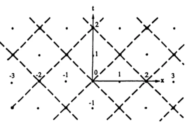
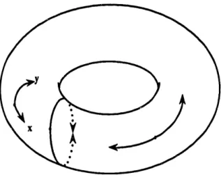
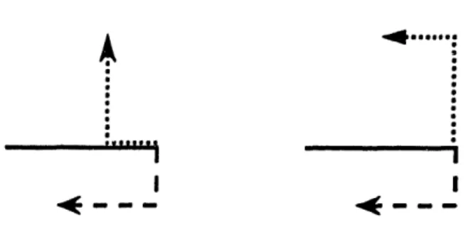
\ .Figure 1: Two-dimensional discrete space-time is decoupled into two distinct lattices for a certain value of the speed of light; the diagonal arcs shown connect the nearest-neighbor points of one such lattice. Higher dimensional space-times are likewise decoupled into two
lattices.
done throughout. In particular, because of the cancellation of all terms in the above equation corresponding to the central term of the right-hand side of (1), the space-time is decoupled into two distinct lattices, even and odd (Figure 1), such that every space-time point (x, t) in the even (odd) sublattice has the property that
n
t+Zxi
(3)
i=1
is even (odd). Without loss of generality, it will be assumed that the solutions con-sidered here are nonzero on only one of these lattices, unless stated otherwise.
It can be seen from the two preceding equations that solutions of the discrete wave equations form a vector space whose dimensionality is equal to twice the number of points in the lattice (i.e., the sublattice). An element of this space of solutions is completely determined by arbitrarily assigning values on all points of the lattice at two successive times.
Any solution of the n-dimensional discrete wave equation defined on an n-cubical lattice of Nn points may also be given in terms of harmonic solutions via Fourier
analysis, e.g.,
n N-1
(xt)=1 ii EA( )e2'(Z+W), (4)
j=l .,=0
where the A(K) depend on the initial conditions. The frequency w, whose functional dependence on the components of Ki has been suppressed for clarity, is given by the
dispersion relation
sin w 12 s E - sin (5)
2 n 2 2
This passes in the continuum limit to the familiar
2 2
k2 = 2 + *- +
k)
(6) where the k, and ky are the respective conjugate variables of the Fourier integral appearing in the continuum generalization of (4). Note that if c2 = 1/n as impliedabove, the numerical integration of (2) is stable. If one were to make the apriori simpler choice of setting c2 = 1, or indeed to any value greater than i/n, then
for all except the one-dimensional case, there would be spatial frequencies for which the modulus of the right-hand side of (5) would be greater than one. The time frequency w would then have to contain an imaginary component in order for the equality to hold, leading in general to an exponential growth of the solutions. As it is, the solutions retain the characteristic undamped periodicity of their continuum analogues. Moreover, their deviation from the continuum case stays bounded. Of course, only solutions whose associated wavelengths are much larger than the lattice spacing can be well approximated by such discrete analogues, but in principle the correspondence may be made as close as desired.
2.1
The one-dimensional case
Traveling waves and arcs
equa-tion may be written as the sum of two traveling waves,
+(X, t) = f+ () + f (),
(7)
where these two traveling waves are respectively functions of the single variables
u = x - t and = x + t, so that they translate unchanged in opposite directions as time passes.
Indeed, this propagation from one space-time point to its neighbors suggests that these traveling waves are functions more naturally defined on the arcs that may be said to connect neighboring space-time points (cf. Figure 1); however, the utility of such a view becomes fully manifest only in higher dimensions. Let fn(x, t) and
fin(x, t) denote functions, which will be referred to as flows, defined on arcs connecting
space-time points of the form (x 1, t - 1). At the risk of redundancy, let fut(x,t) similarly denote functions defined on arcs connecting space-time points of the form (x ± 1,t + 1). Obviously,
f'n (x,t) fut(x
T
1,t-1)
.(8)
The decomposition of (7) then implies
fin(x, t) = ft((x,t).
(9)
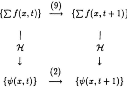
Any solution of (2) may then be expressed in terms of functions defined on the arcs. Like the set of point solutions, the set of arc solutions also forms a vector space, and the traveling wave decomposition implies that there exists a homomorphism from the arc solutions to the point solutions (Figure 2). Moreover, this homomorphism is preserved over time, under the respective time evolution of each system. By the implicit use of this homomorphism, (7) may be restated as
b(x,
t) = f (x, t) + fin(x, t) = fUt(, t) + f°ut(x, t) .(10)
The homomorphism is obviously not one-to-one, since by everywhere setting
(9)
(Ef(X,t)
(9)
Ef(xt+1))
l. l
(2)
({f(x, t)) { ((x, t + 1))
Figure 2: There exists a homomorphism Ht from the space of arc solutions to the space of point solutions that is preserved under their respective time evolutions.
where a is an arbitrary constant, one obtains an arc solution that under the ho-momorphism is mapped onto the trivial (i.e., everywhere vanishing) point solution. However, by a proper choice of the basis functions, the expression of a given solution in terms of the flows can (in any number of dimensions) be made unique, so that the relation between the point solutions and arc solutions becomes an isomorphism.
Completeness
In considering the notion of completeness, for any number of dimensions, the space in question is assumed for convenience to be a torus of length 2N in all spatial dimensions, where N is furthermore an even number. Moreover, let all solutions have the property that
x(.
,xi,..) =x-i(..,xl + N...),
-(11)
where the '+' sign in the expression xi + N implies addition modulo N. Therefore, a solution is completely determined by its boundary conditions on the subspace of points for which the xi range from 0 to N - 1. By making N as large as necessary, the desired generality is retained. (Choosing N to be even makes the initialization described below identical, up to a change of sign, for each subspace. Imposing the parity condition (11) excludes the unphysical or uninteresting solutions containing zero frequency modes or terms linear in the time or space variables.)
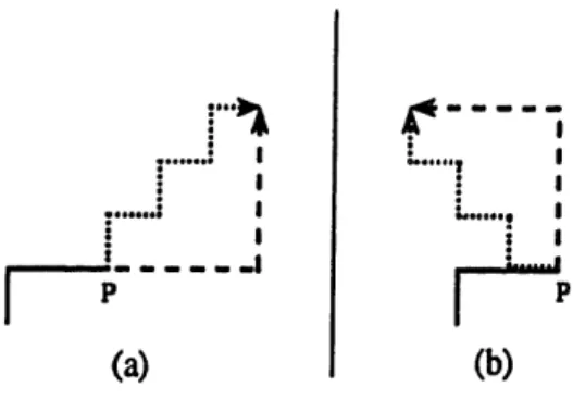
Returning again to one-dimensional systems, let h±(x - xo) stand for the traveling wave solutions that at t = to are zero everywhere except on the arcs going out from the point xo to the respective point x0 ± 1, where they are 1. Such solutions, and
their n-dimensional generalizations, will be called hodotic solutions (from the Greek word for "path"); they have many unusual properties, especially in higher dimensional spaces, some of which will be discussed in the appendix. For purposes of clarity, their time dependence has been suppressed.
A moment's thought will show that under the homomorphism, these arc solutions correspond to the point solutions that at t = 0 are equal to C, 0 and at t = 1 are
respectively equal to , o±l, where 5,, is the Kronecker delta.
Next, let Go(x - xo) and Gi(x - x1), be the point solutions of the wave equation
whose initial conditions (at times to and t = to + 1), are
Go(x -
xo)
= ot,to(12)
G
1(x - xl) = Jx,l6t,tlx, xo,xl E {0,1,...N-1}.
Again, their dependence on time has been suppressed.
It is clear that any solution of the wave equation may be expressed as a linear combination of the Go and G1. On the subspace of length N mentioned above, The
function Go(x - xo) and Gi(x - x1) may be expressed in terms of the arc functions
h+ and h_ as
1 N-2
Go(x - o) = E {h+(x-o -
x')Sgn(x
-xo)x'=0,2,... - h_(x - o - x')Sgn(x - xo - 1)} (13a) and 1 N-1
Gl(x- x
1) =
2
{-h+(x-x
-
x')Sgn(x'- x)
x'=1,3,...+ h_(x - xl- x')Sgn(z' - x)} ,
(13b)
Figure 3: An arrangement of hodotic sohltions that yields a Green's function G(x - l)
for the discrete wave equation. where
Sgn(x) =
{
1
> -1 otherwise.Again, note that if to is even (odd), then the solutions in question are assumed to be nonzero on the even (odd) sublattice; likewise, it is assumed that o is even (odd), while xl is odd (even).
As the equations show, these Green's functions for the discrete wave function may be constructed by interlocking positive and negative hodotic solutions of opposite sign (Figure 3). Therefore, the traveling waves completely suffice to specify the solutions of the wave equation.
Note that these Green's functions require nonzero flows across the entire space. Therefore, even if the solution one wishes to simulate is initially nonzero only in some localized proper subset of the space say, one that can be covered by a line segment (or in n dimensions, an n-cube)-its expression in terms of the Green's functions involves nonzero flows in a region extending across the entire space. However, if this (point) solution satisfies the additional property that its discrete integral over space is constant (as (2) implies it would be if it is the same at any two successive times), then one can find an arrangement of hodotic solutions that is also nonzero only in a localized subset.
2.2
The two-dimensional case
In passing to the two-dimensional case via the present analysis, solutions of the wave equation are again to be expressed as a linear sum of components. Each of these
components will likewise be associated with flows along the arcs connecting nearest neighbors. However, since in higher dimensions even a localized wave packet spreads and deforms, it is to be expected that there will be mixing among these modes of propagation, instead of the trivial translation found in the one-dimensional case.
At any time, let each lattice point be viewed as a kind of black box, into which enter and from which exit four amplitudes. The latter are to be determined solely in terms of the former, in a linear fashion. If, as in the one-dimensional case, the flow out from the point (,y,t) and in to the point (x + 1,y,t + 1) is denoted as
fo+t(x,y, t), or equivalently as f+ (x + 1,y,t + 1), and the flows, to other points are
analogously denoted, these considerations may be restated as
((x, y,
t)
= Ef
f(x, y,t)
= E fout(zx y, t) , (14) andfaut = fi a ,Co , (15)
at
where a, a' E {x+, , y+, y_}, and where the coefficients of the matrix cJ',, are to be
determined.
Consider the solution of the wave equation corresponding to a nonzero flow in only one arc, say, fir (O,0, 0) = 1, with all other incoming flows to all other points being zero; i.e., a two-dimensional hodotic solution. As in the one-dimensional case, the boundary conditions for the corresponding point solution are are b(x, y, 0) = b,oo,0 and (sx, y, 1) = ,1,o.
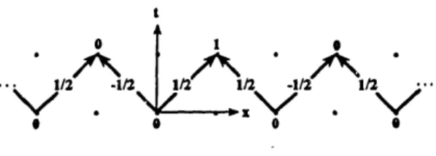
Since the wave amplitude is thus specified on the entire space at two successive times, one can iterate these boundary conditions according to the wave equation (Figure 4), and thus uniquely determine the first column of the matrix cn,,. Repeating
1/2 1/2 -112 t=2 t=l t=0 I 1
Figure 4: The x+ hodotic solution, at t = 0, 1 and 2.
this analysis for the hodotic solutions of the remaining three directions completes the specification of the matrix, showing that
f)z
1 1 1
(
)
(16)By using the time invariance properties of the wave equation, one also could have just as easily determined the coefficients oi the inverse of the above matrix, c°t,, and would have found them to be identical. It is then a matter of algebra to show that the sum of the ingoing or outgoing flows at any point does indeed obey the discrete wave equation.
Note that the sum of the coefficients along any column of the matrix is one, so that the sum of flows entering a point at any time is equal to the sum of the exiting flows. This is also obvious from (14). Furthermore, the matrix is unitary, so that the sum of the squares of the entering (and thus the exiting) flows is conserved. Thus the evolution of such a system can be viewed as a network flow of a conserved quantity.
1/2 Y,'J4 X **114 1 ;011 AV >. _7 -/0-0000" cc v
2.3 Higher dimensional cases
In higher dimensions, the hodotic solutions hi;(x - xo, t) are defined (in terms of their point values on the lattice) by the initial conditions
h. (x - xo,t)=
6,
x,xO sei
for t = to
for t = to + 1
where the jth component of ei has the value 6i. In terms of their arc amplitudes, the hodotic solutions are initially equal to unity on the xi: arc leading out of the point xo, and zero on all the others.
The suppositions (14) and (15), and subsequently utilizing the associated hodotic solutions in order to determine the coefficients of the transition matrix, can be readily generalized to higher dimensions. For example, in three dimensions, the transition matrix is determined to be out 1 1f n x+, 1 -2 1 1 1 1 f fx_ - -2 1 1 1 1 I fv+ I 1 1 1-2 1 1 (18) fV_ =3 I 1-2 1 1 1 (18) k 1 1 1 1 1-2 1 f.
In the general n-dimensional case, the coefficients of the matrix in any row or column will be 1/n, except for the coefficients connecting oppositely directed flows, (e.g., c+,,_), which will be -(n - 1)/n.
In each case, the number of traveling waves is determined by the number of adja-cent neighbors of the points of the lattice, and the evolution of a given wave may be determined by the study of the corresponding hodotic solutions.
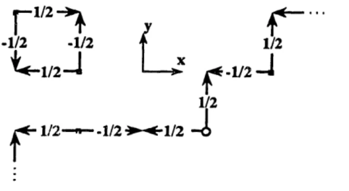
The considerations of completeness may be directly generalized to higher dimen-sions merely by imbedding the one-dimensional expresdimen-sions for the Green's functions (13) along any of the axes. This is arguably the simplest way to express the Green's functions, although in higher dimensions more elaborate expressions are possible (Fig-ure 5), since the overcompleteness of the hodotic solutions is more extensive.
-1/2 -1/2 ~ 1/2
< 1/2 -112
1/2
f1/2-
-- 1/2 -1/2
Figure 5: A two-dimensional non-collinear arrangement of hodotic solutions that yields a Green's function for the discrete wave equation. Nearest-neighbor points are displaced by one unit of time. The circle marks the support of the point solution.
It is possible to formally extend the notions of traveling waves to non-orthonormal lattices, generalizing the discrete wave equation to hexagonal, tetragonal, 6r indeed to any set of points where each point j has some privileged subset .f(j) of generalized nearest neighbors; the "wave equation" then becomes
(j, t + 1) + b(j, t - 1) .A(j) j'EN() (19) where IJ/(j)I is the number of nearest neighbors-not necessarily constant throughout the space-corresponding to the point j. Again, each pair of neighbors will induce a flow, with an interaction among flows that may be determined by studying the behavior of the associated hodotic solutions. As before, there will be a conservation of the sum of the flows, and also of the sum of their squares, since the transition matrix is in all cases unitary. Of course, how well, if at all, the resultant system mimics the continuum wave equation in some limit depends on the particular lattice employed and, if definable, the associated dispersion relation. S. Gudder has studied even more general systems of flows on lattices and graphs, subject only to the condition that the transition matrix at each lattice point or graph node satisfies a unitarity condition[2].
Effective dimensionality
As an aside, note that the discreteness of lattice systems allows the number of dimensions to be easily manipulated in order to apply the above results to other systems of equations. Consider an orthonormal toroidal lattice, as before, and suppose the number of dimensions n, is very large, but that all except m dimensions are exactly one unit long. This means that for all but the first m dimensions, the arcs and flows leading out of a point will lead back in to the very same point. That is, the origin and terminus of such an arc are one and the same. This also means that the even and odd parity sublattices are now one and the same.
In effect, such a system is rn-dimensional; however, the speed of light is still \/i rather than v/im, and the number of types of flows is likewise equal to twice the actual dimension n, rather than m.
The utilization of such systems with "thin" dimensions is a very useful maneuver, and will appear again in the study of the Klein-Gordon equation. Note that the addition of these spurious dimensions does not change the fact that the associated difference equations are numerically stable, and that the Fourier frequencies are al-ways real. Trivial modifications of the above equations also allow one to extend the above results to spaces containing perfectly reflecting or absorbing obstacles, as well as to situations in which the speed of light, or alternately, the index of refraction, varies throughout the space. The appendix will discuss how to generalize the re-sults obtained for the scalar wave equation to the Klein-Gordon, Maxwell, and Dirac equations.
3 Path summations
The same Monte Carlo (and related) methods that are commonly used to simulate diffusion phenomena [3-8] may be extended to the simulation of the wave equation, using the results of the previous section. Such an approach is to be distinguished
from the related method of simulating lattice-wave solutions by density variations of lattice gases [4,11]. The validity of such an approach may be examined by way of the associated (linearized) Boltzmann equation [3-8,10-12]. While it is also possible to obtain a cellular automaton model of the wave equation directly and without recourse to path summations and diffusion phenomena [13], the present approach is more easily estensible to the study of Klein-Gordon and related equations relevant to physics.
We briefly recapitulate some results of the random walk as applied to the diffusion equation, in order to emphasize the similarity of that formalism to the present one. The exposition given here is presented in such a way as to anticipate and facilitate its subsequent application to the wave equation.
Consider a discrete dynamical system consisting of particles executing random walks on an orthonormal n-dimensional lattice. Henceforth, such particles will be referred to as tokens, to distinguish them from the particles whose wave functions will later be simulated by a gas of such tokens. At any step in the (discrete) evolution of the system, tokens are to be found at some lattice point, and they move to a randomly chosen nearest neighboring point in the subsequent time step.
The probability that a token initially at the lattice point xo will at time T be found at x may then be written as
Prob(x; TI xo; 0) =
>
W(I) , (20)I
where I is an indexing of the set of (2n)T lattice paths originating at x0o, ending at
x, and containing T steps. If one assumes that the probability pj± for taking a step along a given direction zj, is everywhere constant, then the weighting factor W(I) has the value
W(I) = (p'+)r,+(l)(pj_)r_(I).. (p. )r_+(I)(p Urn_(I) (21)
where ri, (I) is the number of steps along the xi, direction that are found in the Ith path.
In the case where all the pi, are equal, the right-hand side of (20) can readily be shown to converge in the continuum limit to the kernel for the n-dimensional diffusion
equation [14].
Lattice ensembles
One can use (20) to give diffusion phenomena a statistical implementation. By using an ensemble of appropriately initialized lattices (with the initialization proce-dure to be discussed below), one can use the distribution of tokens on these lattices to simulate a solution of the diffusion equation f(x, t). Like any solution of the wave equation that is to be simulated via the present formalism, f(x, t) is assumed to be approximately constant over the length of the lattice spacing (and over any time inter-val the length of the fundamental time increment). It is also assumed to be bounded, normalized so that its maximum value is initially unity, and for now, positive.
Let the number of lattices in the ensemble be some very large number M. Define
nj(x) to be the number of tokens at the point x at time t in the jth lattice, where j.
ranges from 1 to M, and where the time dependence will customarily be understood. To say that at time t the statistical amplitude at x is f(x, t), is to say that
M
f(x, t) = -
En
j(x),
(22)
regardless of how the occupation numbers vary from lattice to lattice. Likewise, it will be said that an ensemble of lattices statistically simulates the function f(x, t) if the above relation holds. (In any practical implementation, the above equals sign must be interpreted to mean 'approximately equals, to the desired degree of accuracy.')
Initialization
Next, consider how to initialize the ensemble of lattices corresponding to f(x, 0), beginning with the following definition. Performing an action A 'with probability p' is defined as first obtaining a random number ¢, uniformly distributed between 0 and 1. If ¢ < p, then action A is performed; otherwise, it is not. The random numbers
( obtained from multiple repetitions of such actions are assumed to be statistically independent.
Each lattice of the ensemble is to be initialized independently of the others. At point x of say, the jth lattice, one places a token there 'with probability f(x, 0)'. One then repeats this procedure for every other point of the lattice.
Every lattice in the ensemble, with j ranging from 1 to M, is initialized in this same way. This of course means that in general, there will be more than one token per lattice. (Indeed, one could in this case have chosen simply to place the tokens from all the M lattices onto one single lattice, but again, the exposition given here is made in such a way as to facilitate its application to the wave equation.)
Let us suppose that at time T, an ensemble of lattices statistically simulates
f(x, T). In each subsequent time step, let each token move to one of its 2n nearest
neighbors, the choice being made randomly for each token. Assume there is no restriction on the number of tokens that can be found at a given point on any lattice.
By using basic probability theory, one may use (20) to show that an ensemble of lattices initialized according to the preceding procedure will continue to statistically simulate f(x, t) at each subsequent time step. In order to simulate phenomena lasting
T time steps, a number of lattices on the order of (2n)TM will be required in general,
where AM0 is the number of lattices required to initially statistically simulate a given solution to the desired degree of accuracy.
Extensions to complex solutions
There is, of course, nothing about the diffusion equation that requires the solutions to be real. Suppose that each lattice token is endowed with an additional degree of freedom corresponding to a discrete phase factor, having one of the four possible values of 1, +i. -1, and -i; tokens in these respective phases will respectively be referred to as being positive, posimaginary, negative and negimaginary.
Assuming that at the lattice point x of the jth lattice there are a positive tokens, b
of the occupation number nj(x) be modified so that
nj(x) = (a - c) + i(b- d) ; (23)
therefore, this 'occupation number' is now in general a complex integer. Because a, b,
c, and d appear in (23) only as the differences (a -c) and (b-d), the statistics will not
change if oppositely phased tokens (positive vs. negative, posimaginary vs. negimag-inary) found at the same arc are assumed to annihilate each other, leaving behind tokens of at most two phases; this assumption will be made throughout.
One can then use ensembles of lattice tokens to statistically simulate complex solutions as well. To initialize the ensemble of lattices to correspond to the solution
f(x, t), where f(x, t) may now be complex, one first defines the four positive functions:
fRe(X,
t)=
-1±2
U(f))Re[f(x,
t)]
fim+(x, t) = l+S±(f(xt)) Im[f(x, t)],
(24)
after which one simply initializes the ensemble according to each of the four functions simultaneously, in each case using the correspondingly phased tokens; positive tokens for f,+, posimaginary tokens for fin+, and so on. (It is assumed that f(x, 0) has been normalized so that none of the maxima of the above four functions exceed unity.) Therefore, at the end of this initialization every lattice will in general contain all four kinds of tokens, though at any given point on the lattice there will be tokens of at most two phases.Applications to the wave equation
To statistically simulate a solution of the wave equation, one must first expand the point solution (which as stated previously, is specified by its values on the points of the lattice at two subsequent time steps) into an arc solution, by way of the Green's functions (13). It is convenient to normalize the solutions so that the (discrete) integral of the squares of the arc amplitudes is unity, i.e.,
E
I
1(x,t)
2 = 1, (25)given that this quantity is conserved. (The summation indices denote that the sum-mation is taken over all the nearest neighbor arcs of the lattice.)
Then, one initializes the lattices as in the case of the diffusion equation, except that instead of placing tokens at a point x-with a probability and phase dependent on the amplitude at that point--one now places tokens in the arcs leading out from x, in likewise accordance with the amplitude at those arcs. A token in the a arc of the point x will then be assumed to execute a step in the a direction in between the times t = 0 and t = 1, where the 2n possible values of c again represent positive or negative directions along the axes of the lattice.
Just as in the above section dealing with traveling wave solutions, the lattice points should here again be viewed as black boxes, into which tokens enter, and out of which other tokens are generated. Explicitly, the dynamics is such that a token taking a step terminating at some lattice point will cause that lattice point to generate tokens in all the outgoing arcs (with probability distributions to be discussed below). In other words, the token numbers will no longer be constant, so that it is only by averaging that one recovers the conservation of amplitude and its square that is implied by the unitarity of the transition matrices.
The tokens in the outgoing arcs will in the subsequent time step travel along those arcs to the corresponding nearest neighboring lattice point, where the generating process will be repeated. (The parent token is assumed to annihilate after reaching its destination lattice point.)
Consider next the transition matrices for the n-dimensional generalization of (15). Let Ic,,,,l designate the probability that a token coming into a lattice point along the
' arc will produce an outgoing token in the a arc. If c,,,, is positive, then the
outgoing tokens will have the same phase factor, or sign, as the incoming tokens. If it is negative, the outgoing tokens will have the opposite phase of the incoming tokens. For example, in the two-dimensional case (Figure 4), a positive token coming into a lattice point along the x+ arc will produce 'with a probability 1/2' a positive token in the y+ (or y_) arc. It will also produce produce 'with a probability 1/2' a negative
token in the x_ arc, this change of sign being mandated by the fact that the coefficient cx_',+ is negative. The generalization to other dimensions is straightforward.
It is assumed that a parent token generates output tokens in the outgoing arc a completely independently of the tokens it produces in any other arc a'. Moreover, if there is more than one token entering a lattice point, the tokens emitted because of incoming token A are generated independently of the tokens emitted because of some other incoming token B. (Once the tokens are generated, it is again assumed that oppositely phased tokens found simultaneously in any arc annihilate each other.)
An ensemble of lattices that initially simulates the wave equation will then con-tinue to do so in subsequent time steps, as may be shown by the same calculation as in the case of the diffusion equation. If an ensemble of size M is initialized to simulate the wave solution +(x, 0), then in order to obtain the (point) solution at any other time T, one allows the ensemble of lattices to evolve for T time steps and then obtains the quantity
M
(1/M)
Enj(x, T)
(26)
j=1
where nj(x, T) now refers to the sum of the occupation numbers for the arcs leading into the point x (at time T in the jth lattice). Again, simulating phenomena lasting
T time steps to within an initially prescribed accuracy will require a number of
lattices on the order of (2n)TM, where Mo is as before. Note that even though the wave equations are time-reversal invariant, the dynamics used in their simulation are asymmetrical with respect to time-reversal, and it is only by averaging that the symmetry is recovered.
The relationship between amplitudes and paths on the lattice that exists in the case of the diffusion equation may be retained in the present case. A token coming into x along the a arc that produces an outgoing token in the o' arc still specifies a path increment; any token generated in another outgoing arc likewise represents the increment of yet another path. Given that in the general n-dimensional case the coefficients of the transition matrices are 1/n and (1 - n)/n, one may heuristically
say that the (generalized) probability of a token making a path increment along an incoming arc a to an outgoing arc a' is 1 /n, unless the two arcs are oppositely oriented (implying that the associated path increment is a 'reverse step', or reversal), in which case it is (1 - n)/n.
The relation (20) has an analogue in the case of the wave equation, in that the hodotic solutions (and, given the completeness thereof, any solution of the wave equation) can similarly be expressed in terms of summations over paths. In fact, in accordance with the considerations of the previous paragraph, the n-dimensional hodotic solution has the likewise expansion
ho(x
-
xo,
T) =
EW(Is)
(27)
I.
where the 2n possible values of a again represent positive or negative directions along th: lattice, and where I, is an indexing of lattice paths of length T whose initial step is along the a direction. In the present case,
W(I,)
= (1/n)T( - n)R(I) (28)where R(I) is the number of reversals in the path I; for the one-dimensional case
n = 1, zero to the zeroth power is defined to be one.
Thus, there exists a statistical representation of the flows and traveling waves of the wave equation. The path summation formalism is retained, except that the paths are converted into chains of causality with the result that the Huygens picture of wave propagation, whereby any portion of a wave itself emits a wavelet, is likewise given a statistical rendering.
4 Quantum Mechanics
The lattice systems considered here, with their ability to reproduce wavelike phenom-ena by way of discrete particle motions,::provide a novel way of simulating quantum mechanical systems, as the present section will show. As a first step, a lattice quantity
will be introduced whose expectation is equal to the absolute square of the wave func-tion under considerafunc-tion, and which is additive in the number of ensemble members. Initially, the wave functions will for convenience be assumed to satisfy the lattice wave equation, so that they can be interpreted as the wave function of some massless and spinless particle; moreover, the discussion will at first be restricted to one-particle systems.
Bilattices
The phased tens ;used in the previous section to statistically model a solution to the wave equation ~b can obviously be used to obtain the square of the solution as well. However, by using two independent sets of tokens-one to represent
4p
and one to represent b*--it is possible to obtain bIl2 in a more direct fashion, with theduality between the two sets of tokens being in direct correspondence to that which exists between the bras and kets of Dirac's formalism.
Consider again a lattice that has been initialized to simulate some wave function O(x, 0). Next, use a differently labeled, but otherwise identical set of tokens to initialize the identical wave function on that same lattice- note that because the initialization procedure is nondeterministic, the actual configurations of the two sets of tokens on the lattice will in general be different. The first set of tokens will be referred to as bra tokens, the other as ket tokens, and the lattice containing these two types of tokens will be called a bilattice.
Let ii(x) refer to the (complex) occupation number, as defined above, obtained by counting the ket tokens in all the arcs leading into the point x; similarly, let (x) refer to the occupation number obtained by counting the bra tokens on the same arcs. The motion of the bra tokens is totally independent of that of the ket tokens.
Event counting
Although there is no direct correspondence between lattice tokens and the particles of matter whose wave functions are being simulated, there does exist a quantity,
expressed in terms of the location of tokens at a lattice space-time point, whose expectation is equal to the probability of finding a matter particle at the corresponding space-time point i the physical space being simulated.
By way of analogy, the simultaneous presence of any bra token and any ket token at some lattice point x will formally be referred to as a one-particle event, for reasons which will become clear below, and will be denoted as e(x) (the time dependence is suppressed for clarity). Taking the summation of such events over an arbitrary set of lattice points will likewise be referred to as a one-particle event count, even though the increments to this count need not be positive, and may have an absolute value greater than one. Every event has a phase factor associated with it, which is defined to be the phase factor of the ket token times the complex conjugate of the phase factor of the bra token, and the event count is incremented algebraically according to the phase of the respective events. Thus, if A denotes a bra token and B denotes a ket token, one may express the phase factor of the event for which a bra token A and a ket token B arrive at x as
Ph[e(x)] = Ph[A]'Ph[B] (29)
Typically, the distinction between e(x) and the weighting factor Ph[e(x)] will be ignored, and the former expression will be used to designate the latter. If j bra tokens and k ket tokens arrive at some space-time point (x, t), they collectively represent jk distinct one-particle events, so that one may write, by way of definition,
i e(x) -h (a(x), (30)
where the summation is over all the one-particle events at x (and t). Now the initial-ization of bra tokens is statistically independent of the initialinitial-ization of the ket tokens. Therefore, on any bilattice which has been initialized to simulate the wave function i(x, 0), it is the case that
where the count has been taken at t.
Note that bra and ket tokens will increment the event count taken at a given point even if they do not come into that point on the same arcs, so long as they are both on the same bilattice. A,so note that since the expected value of the event count is
always real, one may as well ignore any events having an imaginary phase, so that with such an understanding, the results of the event count can be considered a real quantity.
Let ht,(x) denote the occupation number of ket tokens found in the a arc in a bilattice leading into the point x, and ih(x) likewise denotes the complex conjugate of the bra occupation number of that same arc. It then follows that the expected value of hi,(x)i,(x), when integrated over all the arcs in the bilattice, is conserved, due to the unitarity of the transition matrices. This quantity is to be distinguished from the expected value of the summand in (30). The latter is obtained by considering tokens arriving at points, and its discrete integral over time varies, while the former (constant) quantity is obtained by considering the location of tokens on the individual
arcs.
Diffraction
One can of course initialize bilattices to simulate to a wave packet of some well defined momentum. Consider the following double-slit diffraction experiment such as is found in standard introductory quantum mechanics texts. Imagine placing in the bilattice a screen, facing orthogonally to the momentum of each wave packet. Assume the screen contains two parallel slits having widths on the order of the mean wavelength of the wave packet, with the slits being separated by a distance smaller than the coherence length of the packet. Any convenient boundary conditions may be imposed on the slits-for example, those corresponding to perfect absorption.
Consider making an event count at some observation point x on the opposite side of the screen at some distance that is large in comparison to the widths of the slits, and which a lattice particle can only reach by propagating through those slits.
Quantum mechanics tells us that the probability of a particle being found at a point x of the observation screen at some time t is
0iI(X) + I(X)I ,
where bI is the amplitude whose square would determine the probability of a particle arriving at x if only slit I were present, and so on. The time dependence of the wave functions will be understood.
Suppose that a large number of identical lattices are initialized to simulate some function i(x). Consider the event count taken on all the points corresponding to some point x for which complete cancellation occurs, i.e., where the amplitude associated with one slit totally cancels the amplitude associated with the other.
Quantum mechanics predicts that in such a region, no particles will arrive. In the present model, however, there are in general many increments in what is called the event count; the result of the count would then be zero (or, more precisely, vanishingly small in comparison to the counts taken in a region of constructive interference) only because positive events are equally likely as negative events.
The absolute square of wave function can be written as
ipI, + 41M)1II + bi~nII + '?0bMI , (31) where the dependence on time and space has been suppressed. Note that the events, i.e., the simultaneous arrivals of a single bra and a single ket token, can be con-ceptually placed into four classes, corresponding to each of the above four terms. Respectively, a token from the first class represents events in which both the bra and ket token came through slit I; the second, an event for which both came through slit II; the third, an event for which the bra token came through slit I and the ket came through slit II; and the fourth, an event for which the bra token came through slit II and the ket came through slit I. (Saying that the bra token of a certain event came through a certain slit means that the chain of interactions that led to the token's
arrival at the observation point define a space-time path that leads through that par-ticular slit. Note again that several tokens can be found at any bilattice arc, each one being associated in general with a distinct path.)
Depending on how the slits and the observation points are situated, one may recast all the features of the particle diffraction gedankenexperiment in terms of event counts obtained on the ensemble of bilattices. For example, shutting one of the slits, or slightly perturbing the tokens exiting from either slit can block the arrival of certain events, or destroy the coherence evidenced by the third and fourth terms in the above expression.
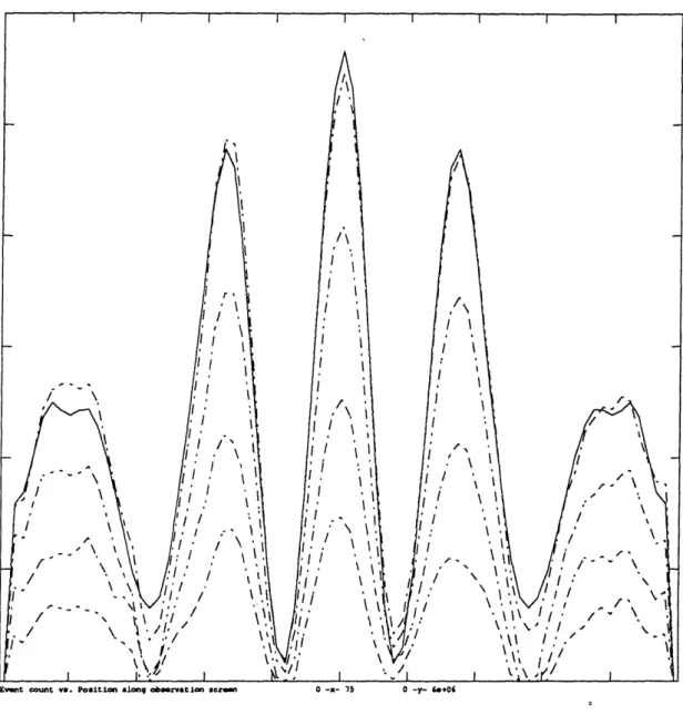
The interference patterns shown in Figure 6 were obtained by simulating a double-slit diffraction experiment by way of the discrete, statistically implemented two-dimensional lattice wave equation (2). The dimensions of the bilattice are 33 x 75 units, with the observation screen, i.e., the line of points along which the event counts are taken, being oriented along one of the long edges of the bilattice. On the edge opposite to the screen are the one-unit-wide slits (i.e., the emission points) which are situated ±10 units from the center. The wave packets, which were each given the standard normalization indicated in (25), were such that their contributions to the bra and ket occupation numbers at the slits were integers whose expected values varied sinusoidally, with a period of 10 time steps. The total time duration of each packet was 50 time steps. The nondeterministic evolution of the token occupation numbers at any arc was obtained simply by iterating the arc amplitudes at any time step according to (16) and then incrementing any resultant half-integer occupation number by a random choice of ±1/2, thereby ensuring that the token occupation numbers were always integers. The remaining boundary conditions were such as to correspond to total absorption of the tokens at any of the lattice's edges:
The four dashed lines show the event count distribution after the emission of 50, 100, 150, and 200 million "photons", respectively, with the abscissa ranging along the one-dimensional observation screen, from 0 to 75. Each tick on the ordinate axis
Evet count v. tPo.ti &lon obseration ceen 0 -- 75 0 -y- X+06
Figure 6: Interference patterns obtained in a two-dimensional double-slit diffraction exper-iment. Dashed lines show the event count distributions subsequent to the emission of 50, 100, 150, and 200 million "photons", as a function of position along the observation screen. The solid line indicates the exact solution of the interference pattern corresponding to the lattermost event count distribution.
corresponds to a million events. The solid-line graph-which has been normalized so as to have the same integral as the graph corresponding to 200 million photons-shows the exact solution of the interference pattern, obtained by integrating (2) with real (as opposed to integer) arc amplitudes and emissions.
Note for future reference that it is possible to make the amplitudes in even this discrete formulation quasi-continuous by assigning each bra and fet tken a fractional weight of y, where a is a small positive number. Then the arrival of a bra and ket token
would only increment the eveit count by a factor of ±72, where the sign depends on
the phase of the tokens. As the value of 3' is made to approach infinitesimal values, the amplitudes take on quasi-continuous values; nevertheless, as will be shown, the way in which the mass and potential terms are incorporated into the formalism implies that the amplitudes are ultimately best considered as discrete entities rather than continuously varying quantities.
4.1 Multi-particle phenomena
Consider next the simulation of multi-particle phenomena.
Assume for now that all the particles (as opposed to tokens) being simulated are indistinguishable, and are fermions; the case of simulating bosons will follow straightfor:ardly. Although the systems under consideration in this paper are rel-ativistically covariant (in the continuum limit), the number of particles will still be a good quantum number in the absence of interactions, so that it is permissible to speak of multi-particle states containing a fixed number of particles.
In considering multi-particle wave functions, it is necessary that the tokens cor-responding to different one-particle states be distinguishable from the tokens corre-sponding to another. There are a number of ways to impose this distinguishability, some more physically plausible than others, but for the sake of the presentation, it is simplest to assume that the tokens corresponding to different states are distinguished by a label or a tag of some sort, which shall be referred to as a particle index. In fact,
this particle index can be viewed as a sort of rudimentary momentum, given that it represents an extra degree of freedom that a particle may assume. However, it does not influence the dynamics of a token. The range of the particle indices, i.e., the number of distinct values they can assume, needs to be only as large as the number ot one-particle states that are being simulated.
Initialization
Consider the Slater determinant of the N one-particle states
1bl(x),
... , cN(X) by way of which the N-particle wave function is expressed in terms of its one-particle state constituents Oi(x), with i ranging from 1 through N, as(Xl,...
-
,XN) =Z
p[1](X1l)" b p( p[v(xN)a(P) (32)where P is some permutation of the numbers lthrough N, the sum is over all such permutations, and o(P) is 1 or -1 according to whether the permutation is even or odd. (Again, the time dependence of the wave functions has been suppressed.)
To initialize a lattice to simulate such a wave function, one can proceed as if the wave functions possessed no particle exchange symmetry. That is, the wave function is initialized according to one of the N! terms in (32); the symmetrization will ultimately appear as a result of the way in which the count is taken.
For convenience, consider initializing a lattice according to the wave function
X (X1)2 (2) - N (XN) (33)
In doing so, each one-particle wave function is to be initialized independently; more-over, all the tokens used in initializing j(xj) will have identical particle indices, that are distinct from those used in initializing some other state Ok(Xk). Therefore, pre-suming that the single-particle wave functions will in general overlap, each arc will be allowed to contain tokens with differing particle indices. Later on, it will be shown that for fermion states, the number of distinct particle indices at any single arc can
be reduced to one. For now, it will be assumed that only oppositely phased tokens with the same particle index are allowed to annihilate.
An N-particl; event (where N need not equal N) is then defined as the simul-taneous arrival o N/ 'distinctly labeled tokens at the observation points x1, x2, ...,
xg, along with the arrival of N ket tokens, subject to the restriction that the particle index of the ket token found at xi is the same as that of the bra token at xp(,), where
P is some (single) permutation of the numbers 1 through N. Such an event will be
denoted as e(xpl], XP[2],... , xp[/9), or e(P[1],..., P[N]) for short. The phase of the
event is defined to be the product of all the ket tokens' phases times the complex conjugate of the product of the bra tokens' phases, times an additional factor of -1 if P is an odd permutation.
By arguments similar to those considered in one-particle systems, the expected N-particle event counts are such that
N N
e(P[l],...,
PI[I)-
*
* *
E
0! (x,)Oi,
(xp(])
* *
*
, (xi,,)Oi
(xp[,9)a(P)
,
i,=lI if--1 i. i
(34)
where it is assumed that the bilattice in question was initialized to statistically simu-late the N-particle wave function (x 1,x2,... ,XN), as expressed in (33), and where
the summation is restricted to terms for which all the ij are distinct. This quantity is equal to the probability
Prob(xl,
x2,... ,
X)
,
(35)
of finding N particles at the respective observation points times a factor of N!, this factor resulting from the fact that the present formalism yields only the sum of prob-abilities of the form (35) that are identical up to a permutation of its arguments. Alternatively, one could have chosen to distinguish each possible assignment of par-ticle indices to the tokens during assignment.
The validity of (34) is most easily proven by showing that events for which an identically tagged bra and ket particle are located at the respective observation points
xi and xj have an expected value proportional to EN 4,(x)qk(xj). It may likewise
be shown that the above result holds for arbitrary N and N, provided that the summation is taken over all ordered selections (without repetition) of N elements from the set {1,..., N); note that from the definition of multi-particle events, it follows that the expected value of the event count is identically zero in the case where
> N.
As an example, let the diagram
G
B
R
0
Xl X2 X3 X4 (36)
R' O' B' G'
stand for the four-particle event e(4312) in which ket tokens whose particle indices shall be labeled 'green' (G), 'blue' (B), 'red' (R) and 'orange' (O) arrive at the four observation points xl through x4 simultaneously with bra tokens labeled 'red',
'orange', 'blue' and 'green', respectively. The phase of this event is then the product of the ket phases times the complex conjugate of the bra phases, times another factor of -1, because ROBG is an odd permutation of the labels GBRO. Note that while the interchange of any two bra (or else ket) tokens negates the phase of an event, exchanging any two particle indices leaves the phase unaltered, since this is equivalent
to an interchange of both bra and ket tokens.
An N-particle event involving distinguishable particles, say particles of type A and B, will be considered valid if bra and ket tokens of type A constitute a valid NA-particle event and bra and ket tokens of type B constitute a valid NB-particle event, where N = NA + NB. The phase of the event is the product of the phases of the constituent events. Events involving bosons are treated in the same fashion, except that the phase of an event is obtained directly from the bra and. ket tokens, without any extra factor of a(P).
Note that it is possible to initialize distributions of N particles which give a predetermined particle event count while at the same time ensuring that all N-particle event counts for which N < N have an expected value of zero. For instance,
in a 2-particle event initialized with tokens having the particle indices red (R) and blue (B) respectively, consider the operation of multiplying all the R ket tokens by a phase of i and all the B tokens by a phase of i where r and b are integers such that their sum is a multiple of 4. If r = 1 for example, this means transforming all the positive R tokens into posimaginary ones, all the posimaginary ones into negative ones, and so on. A similar transformation is applied to all the constituent bra tokens as well, with some other randomly chosen integers r and b (similarly subjected to the constraint that their sum a multiple of 4). In any ensemble of identically prepared two-particle systems, let this randomization be repeated throughout.
Clearly, any two-particle event count is invariant under such an operation, since the phase of every two-particle event involves the product of the constituent R and B tokens, and this product remains unchanged, for both bra and ket tokens. However, because there is now an essentially random phase relationship between the R bra and the R ket tokens, etc., any one-particle event count will be zero. By modifying the definitions of r and b for either the bra or ket states, one can construct two-particle events whose expected values are negative.
Such anomalous distributions of tokens, and their generalizations, are not sim-ply a mathematical artifice; they are in fact necessary in order to properly initialize systems of particles with internal structure (spin, isospin, etc.) However, since mea-suring such properties involves subjecting the particle states to the corresponding mediating fields-and thereby elaborating the requisite interactions-the utilization of such distributions will be left as a future development.
Coalescing token tags
As mentioned previously, the Pauli exclusion principle allows for a considerable simplification of the token dynamics, in the case of fermionic wave functions.
Consider as an example a two-particle state, for which the particle indices will again be denoted as red (R) and blue (B). Because the wave function at any point corresponding to either of the single-particle states can be written as a sum over
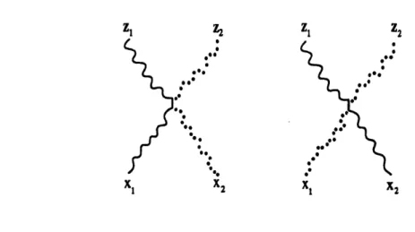
token paths, the product of the two wave functions at any two points may likewise be written as a sum over pairs of token paths. Consider all such pairs of paths for which two distinctly tagged ket tokens are at some time within the same arc. Thus, the R and B tokens may be said to tvel into the same arc, whereupon exiting, the
R token eventually gets to, say, the observation point xl at the same instant as the B token gets to x2 (cf. Figure 7).
Note that because the two tokens were initially on the same arc, the probability of one of them subsequently arriving at a given point with some phase is the same
for both tokens (up to a factor representing their phase differences at the time when they were both in the same arc). In other words, for any pair of paths in which the R token arrives at xl and the B token arrives at x2, there is another equally probable
pair of paths, call it the switched pair, for which the R token arrives at x2 while the
B token arrives at xl, i.e., for which the tokens exchange their paths subsequent to
entering the common arc.
The first pair of paths appears in the path summation expression of +0(x1)x(x2), while the switched path appears in the expression of X(xl)k(x2).
Now any associated event for which the two ket paths have a path step in common is just as likely as an event for which the bra paths are identical, but for which the ket paths are the switched paths. But since a(P) differs for the two events, they will have opposite signs, so that the expected contributions of such events cancel. Therefore, in the context of this model, the effect of Pauli exclusion principle is a cancellation of all events involving the simultaneous presence of distinctly indexed tokens at any arc.
As a result, it is possible to greatly simplify the token dynamics. One cannot simply have such coincident ket tokens of opposite phase annihilate; that would distort the event counts involving only events in which there is, say, only a single bra token with a particle index of R. A similar argument precludes the simple annihilation of ket tokens.
z2 Z, z2
0
.
ie
Xl X2 X X2
Figure 7: Products of hodotic wave functions can be related to a sum over pairs of paths. Any pair of paths which coincide at some arc can be matched with a pair whose steps subsequent to entering the arc are interchanged. The net contribution of such pairs is zero.
found in the same arc, they may be replaced by two tokens whose particle indices are identical. That is, one can have either of the tokens take on the particle index of the other. If there are only two tokens present, then the surviving particle index has an equal probability of being either of the two initial values. In the above example, rather than having an R token and a B token exiting an arc with probability one, there can instead be two R tokens or else two B tokens, each with a probability of 1/2. Therefore, the statistical weight attributable to each of the path steps in question remains unaltered.
In order for this dynamical refinement to produce the proper sign, a token that assumes another token's particle index must also assume the phase of that other token. As an example, suppose a positive R token and a negative B token arrive at a given arc. In that case, the exiting tokens will both be positive, and have the particle index R, or else will both be negative, with a particle index of B; the probability of either outcome is 1/2.