HAL Id: hal-00317364
https://hal.archives-ouvertes.fr/hal-00317364
Submitted on 1 Jan 2002
HAL is a multi-disciplinary open access
archive for the deposit and dissemination of
sci-entific research documents, whether they are
pub-lished or not. The documents may come from
teaching and research institutions in France or
abroad, or from public or private research centers.
L’archive ouverte pluridisciplinaire HAL, est
destinée au dépôt et à la diffusion de documents
scientifiques de niveau recherche, publiés ou non,
émanant des établissements d’enseignement et de
recherche français ou étrangers, des laboratoires
publics ou privés.
Earth’s magnetosphere. 2. Density profiles
H. Laakso, R. Pfaff, P. Janhunen
To cite this version:
H. Laakso, R. Pfaff, P. Janhunen. Polar observations of electron density distribution in the Earth’s
magnetosphere. 2. Density profiles. Annales Geophysicae, European Geosciences Union, 2002, 20
(11), pp.1725-1735. �hal-00317364�
Annales
Geophysicae
Polar observations of electron density distribution in the Earth’s
magnetosphere. 2. Density profiles
H. Laakso1, R. Pfaff2, and P. Janhunen3
1ESA Space Science Department, Noordwijk, Netherlands
2NASA Goddard Space Flight Center, Code 696, Greenbelt, MD, USA
3Finnish Meteorological Institute, Geophysics Research, Helsinki, Sweden
Received: 3 September 2001 – Revised: 3 July 2002 – Accepted: 10 July 2002
Abstract. Using spacecraft potential measurements of the
Polar electric field experiment, we investigate electron den-sity variations of key plasma regions within the magneto-sphere, including the polar cap, cusp, trough, plasmapause, and auroral zone. The statistical results were presented in the first part of this study, and the present paper reports detailed structures revealed by individual satellite passes. The high-altitude (> 3 RE) polar cap is generally one of the most
tenu-ous regions in the magnetosphere, but surprisingly, the polar cap boundary does not appear as a steep density decline. At low altitudes (1 RE) in summer, the polar densities are very
high, several 100 cm−3, and interestingly, the density peaks at the central polar cap. On the noonside of the polar cap, the cusp appears as a dense, 1–3◦ wide region. A typical
cusp density above 4 REdistance is between several 10 cm−3
and a few 100 cm−3. On some occasions the cusp is crossed multiple times in a single pass, simultaneously with the oc-currence of IMF excursions, as the cusp can instantly shift its position under varying solar wind conditions, similar to the magnetopause. On the nightside, the auroral zone is not always detected as a simple density cavity. Cavities are ob-served but their locations, strengths, and sizes vary. Also, the electric field perturbations do not necessarily overlap with the cavities: there are cavities with no field disturbances, as well as electric field disturbances observed with no clear cav-itation. In the inner magnetosphere, the density distributions clearly show that the plasmapause and trough densities are well correlated with geomagnetic activity. Data from indi-vidual orbits near noon and midnight demonstrate that at the beginning of geomagnetic disturbances, the retreat speed of the plasmapause can be one L-shell per hour, while during quiet intervals the plasmapause can expand anti-earthward at the same speed. For the trough region, it is found that the density tends to be an order of magnitude higher on the day-side (∼ 1 cm−3) than on the nightside (∼ 0.1–1 cm−3), par-ticularly during low Kp.
Key words. Magnetospheric physics (auroral phenomena;
Correspondence to: H. Laakso (hlaakso@so.estec.esa.nl)
plasmasphere; polar cap phenomena)
1 Introduction
The modeling of the plasma number density in the magne-tosphere is a difficult task for a number of reasons. First, the total density can significantly change on short temporal and spatial scales as a result of solar wind – magnetosphere – ionosphere coupling processes. In addition, it is difficult to gather reliable measurements of the total density in a tenu-ous environment, and hence, there are only limited amounts of density data reported to date from the Earth’s vast magne-tosphere.
Despite these difficulties, numerous studies of the electron density distribution within the magnetosphere have been re-ported previously. For example, Park et al. (1978), using the whistler wave technique, and Carpenter and Anderson (1992), using in situ measurements, studied the plasma sity within the the plasmasphere. Besides modeling the den-sity inside the plasmasphere, such data sets have also enabled models of the location of the plasmapause to be established (Gallagher et al., 1995).
Beyond the plasmapause, the electron density distribution becomes increasingly complex, especially during enhanced geomagnetic activity. For example, high convection veloc-ities can rapidly change the distribution of the plasma den-sity. Carpenter and Anderson (1992) modeled the plasma trough using ISEE data, and Gallagher et al. (1998) intro-duced a similar model as a function of Kp, using GEOS 2
observations of Higel and Wu (1984). Recently, Gallagher et al. (2000) presented a global plasma model for the entire inner magnetosphere. In general, however, the modeling ef-forts are impeded by a lack of comprehensive high-altitude data sets.
At higher latitudes, the modeling of the plasma density becomes even more complicated due to strong variations on short time scales. Also, the measurements available are quite sparse above 4 REdistances, preventing empirical modeling
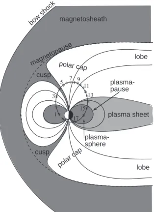
* * * ********* * * * * * * plasma sheet magnetosheath bow shock cusp cusp plasma-sphere magnetopause lobe 1 3 5 7 9 11 13 15 17 plasma-pause polar cap polar cap lobe
Fig. 1. Schematic drawing of the Earth’s magnetosphere in the
noon-midnight meridian. A solid line presents a Polar trajectory; asterisks give the spacecraft’s position at one-hour intervals.
attempts. Persoon et al. (1983) used DE-1 observations to model the density distribution in the polar cap region be-tween a 2 and 4.6 RE distance. Using the same database,
Persoon et al. (1988) investigated the formation of auroral cavities and showed that within these structures, some of the lowest densities within the magnetosphere may be found.
In the first part of this study, Laakso et al. (2002) inves-tigated how the electron density varies statistically in the magnetosphere, using 45 months of satellite potential data from the EFI experiment of the Polar satellite. These data cover 107data points (one-minute averages) distributed be-tween 2 and 9 RE geocentric distances along Polar’s
po-lar orbit. Using high-resolution data from individual orbits, the present paper investigates several plasma regions that have distinct density signatures, such as the polar cap, cusp, trough, plasmapause, and auroral zone. In particular, the ob-servations are used to show how these regions evolve with time and geomagnetic activity.
2 Density variations in the specific magnetospheric regions
We use measurements gathered by the electric field instru-ment (EFI) on the Polar satellite. Polar was launched on 24 February 1996, into a 90◦inclination orbit with a 9 RE
geo-centric apogee distance (initially over the Northern
Hemi-sphere), a 1.8 RE perigee distance (initially over the
South-ern Hemisphere), and an orbital period of about 18 h. The orbital plane rotates about the Earth with respect to the Sun in one year so that all local times are covered in a 6-month period. Figure 1 presents a schematic drawing of the mag-netosphere at the noon-midnight meridian and a Polar orbit, where asterisks mark the position of the satellite at one-hour intervals.
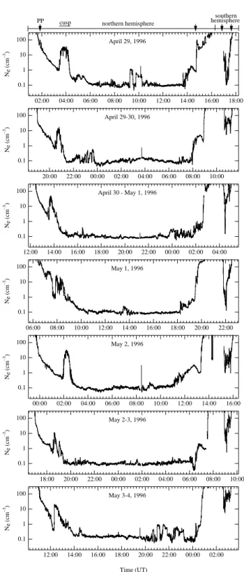
This section presents plasma density profiles in selected regions that are frequently encountered by Polar, such as the polar cap, cusp, auroral zone, trough, and plasmapause. Fig-ure 2 shows the electron densities derived from spacecraft potential data gathered with the electric field instrument for seven consecutive orbits near the noon-midnight meridian on 29 April to 4 May 1996. Each panel displays measurements between subsequent dayside equatorial crossings (see orbit in Fig. 1). In each of the panels in this presentation, the space-craft is first in the high-density plasmasphere, where the den-sity is typically several 100 cm−3 or more, and is moving towards the northern polar cap in the noon sector.
After about an hour, the density decreases a few orders of magnitude when the satellite completes its outbound crossing of the plasmapause (PP). The approximate locations of the plasmapause for the top panel are marked with arrows. A few hours later, a significant, large-scale density enhancement is observed when Polar enters the northern cusp. Poleward of this region, the density becomes very low as the satellite en-counters the polar cap. Polar subsequently moves into the night sector, and at the equatorward edge of the polar cap, it crosses the auroral zone and later the plasmasphere. At the end of each interval, low densities are detected when the satellite passes through the auroral zone and polar cap over the Southern Hemisphere. These encounters are quite short during this portion of the orbit due to the low altitude and high speed of the satellite.
Although the density variations are quite similar from orbit to orbit, there are numerous differences between orbits which reveal fascinating and complex features, such as large-scale density patterns in the polar cap, the structure of the cusp, density cavitation at the auroral zone, characteristics of the density decline at the plasmapause and so on. Their structure and dynamics are revealed to the fullest extent when the data are studied with high time resolution, with respect to invari-ant variables, such as L-shell and invariinvari-ant latitude.
2.1 Polar cap
The statistical study by Laakso et al. (2002), as well as the data shown in Fig. 2, imply that the electron density is very low in the high-altitude polar cap region. The polar cap den-sity strongly depends on season (solar illumination), geo-magnetic activity, and altitude. Next, we proceed with our investigation by studying some individual passes through the polar cap region. As the spatial density variation in the polar cap’s noon-midnight meridional plane is strongly influenced by the positions of the cusp and auroral zone, we use
po-lar cap data from the dawn-dusk meridian for this particupo-lar study.
Figure 3 presents the polar cap density measurements from 1–6 January 1997, versus invariant latitude for both northern winter (at high altitudes, red points) and southern summer (at low altitudes, blue points) conditions. The left panels are for the dawn sector and the right panels for the dusk sector. The bottom panels show the spacecraft distance for the South-ern and NorthSouth-ern Hemisphere passes. If the derived density exceeded 300 cm−3, it was given that value. Recall that our method for deriving the plasma density becomes increasingly unreliable for high electron fluxes (Laakso et al., 2002). Such measurements are useful, nevertheless, as indicators of how often high-density plasmas are encountered.
When interpreting the polar cap measurements of Fig. 3, it is important to bear in mind that the northern polar cap is in a shadow for most of the time, whereas the Sun is continuously ionizing the southern polar cap. For compar-ison, Fig. 4 presents measurements at the same meridian six months later, on 5–10 July 1997, during the northern summer and the southern winter where these conditions are reversed. In the high-altitude (> 4 RE) winter polar cap (see Fig. 3),
the data points are concentrated primarily in the range of 0.01–1 cm−3. The equatorward boundary of the polar cap does not appear very clearly. On the dawnside, the data sug-gest the polar cap boundary may be near 73–75◦, whereas on the duskside a steep decline occurs near 71◦. In summer (see Fig. 4), the high-altitude polar cap density, particularly on the dawnside, is more variable and somewhat higher, ranging between 0.05 and 10 cm−3. On the dawnside, the polar cap boundary likely occurs near 76◦, whereas on the duskside it possibly exists at 70◦.
At low altitudes (∼ 0.9 RE), there is no distinct density
decline at the polar cap boundary in either season. In winter (Fig. 4), the low-altitude polar cap density usually remains below 50 cm−3, the densities are highly variable, with values below 1 cm−3frequently observed. In summer (Fig. 3), the densities are significantly higher, seldom below 10 cm−3and often above 100 cm−3. Furthermore, interestingly, the den-sity is quite constant and higher in the polar cap than at lower latitudes; notice that lower densities above 85◦ are mainly due to orbital coverage. The dawn-dusk asymmetry may well be associated with the IMF orientation and the structure of the convection shell. The investigation of such details are however, beyond this study.
2.2 Cusp
The cusp is the region where the solar wind plasma has di-rect access to the Earth’s environment (Smith and Lockwood, 1996). In the magnetosheath, the average solar wind density is 50–100 cm−3, which is an order of magnitude higher than the solar wind density and two orders of magnitude higher than densities in the outer regions of the dayside magneto-sphere. Thus, the density should be relatively high in the cusp. In fact, this is exactly how the cusp is distinguished in Fig. 2, i.e. as a local enhancement of the plasma density,
0.1 1 10 100 Ne (cm –3 ) 02:00 04:00 06:00 08:00 10:00 12:00 14:00 16:00 18:00 Time (UT) April 29, 1996 0.1 1 10 100 Ne (cm –3) 20:00 22:00 00:00 02:00 04:00 06:00 08:00 10:00 Time (UT) April 29-30, 1996 0.1 1 10 100 Ne (cm –3) 12:00 14:00 16:00 18:00 20:00 22:00 00:00 02:00 04:00 Time (UT) April 30 - May 1, 1996 0.1 1 10 100 Ne (cm –3) 06:00 08:00 10:00 12:00 14:00 16:00 18:00 20:00 22:00 Time (UT) May 1, 1996 0.1 1 10 100 Ne (cm –3) 00:00 02:00 04:00 06:00 08:00 10:00 12:00 14:00 16:00 Time (UT) May 2, 1996 0.1 1 10 100 Ne (cm –3) 18:00 20:00 22:00 00:00 02:00 04:00 06:00 08:00 10:00 Time (UT) May 2-3, 1996 0.1 1 10 100 Ne (cm –3) 12:00 14:00 16:00 18:00 20:00 22:00 00:00 02:00 Time (UT) May 3-4, 1996 northern hemisphere southern hemisphere cusp PP
Fig. 2. Electron density variation on eight consecutive orbits of 29
April to 4 May 1996. The satellite’s orbital plane is near the noon-midnight meridian. Each panel presents a full orbit of data, from one perigee to the next one.
when the satellite moves from the dayside magnetosphere through the cusp into the polar cap (Marklund et al., 1990; Palmroth et al., 2001; Laakso et al., 2002).
Ne (cm –3 ) Ne (cm –3 ) 0.1 1 10 100 Ne (cm –3 ) 0.1 1 10 100 Ne (cm –3 )
Dawnside January 1–6, 1997 Duskside
10 8 6 4 2 0 Distance (R E ) 90 85 80 75 70 65 Inv. latitude (˚) 90 85 80 75 70 65 Inv. latitude (˚)
Fig. 3. Polar cap density plotted against
invariant latitude for 1–6 January 1997. The panels from top to bottom are: elec-tron density in the high-altitude north-ern polar cap, electron density in the low-altitude southern polar cap, and the altitudes of the satellite during the polar cap observations. The red color is used for the northern polar cap and the blue color for the southern polar cap. Here the northern polar ionosphere is in dark-ness and the southern polar ionosphere is sunlit. Ne (cm –3 ) Ne (cm –3 ) 0.1 1 10 100 Ne (cm –3 ) 0.1 1 10 100 Ne (cm –3)
Dawnside July 5–10, 1997 Duskside
10 8 6 4 2 0 Distance (R E ) 90 85 80 75 70 65 Inv. latitude (˚) 90 85 80 75 70 65 Inv. latitude (˚)
Fig. 4. Same as Fig. 3 but for the
inter-val 5–10 July 1997. Contrary to Fig. 3, here the northern polar ionosphere is il-luminated by the Sun and the southern polar ionosphere is in darkness.
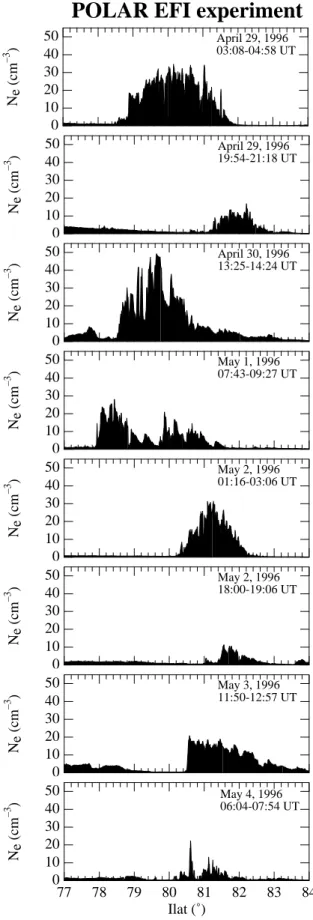
density are highly variable. To illustrate this further, Fig. 5 displays the electron density versus invariant latitude for the cusp crossings in Fig. 2. The thickness of the cusp in these examples varies between 1–3◦in invariant latitude, which is more than that observed with low-altitude DMSP satellites (Newell and Meng, 1992).
Both the location and density of the cusp can significantly
change from orbit to orbit. Although high-altitude cusp
crossings by Polar may last between 0.5–4 h (Palmroth et al., 2001), depending on the satellite’s altitude, in Fig. 5 the crossings last only 0.5–1 h. In the cusp, the average den-sity is usually several 10 cm−3 and can sometimes exceed 100 cm−3, although not in the cases shown in Fig. 5. Note
that such densities are of the order of the magnetosheath den-sity and typically an order of magnitude higher (or more) than in the magnetospheric regions adjacent to the cusp.
Since Polar may spend considerable time crossing the cusp region, the cusp itself may evolve and change dynamically during this time. In the fourth panel from the top in Fig. 5, for example, it seems that the cusp is encountered twice. We have examined the IMF observations from the IMP-8 and Wind satellites during this event and found that simul-taneously with this crossing, the IMF orientation had two large excursions. In fact, Polar has encountered several other events like this, which all suggest that the cusp position is very sensitive to the IMF orientation, and the cusp position
can more or less instantaneously be influenced by IMF vari-ations.
Another common feature in the cusp density profiles is a steep density gradient on the equatorward boundary of the cusp, which is caused by a rapid motion of the cusp over the satellite rather than the satellite’s movement over a stationary cusp (the satellite’s speed is only a few km s−1). Figure 5 shows three exceptions from this common feature, namely the examples in panels 2, 5 and 8 from the top, where the density profiles are quite symmetric, which suggests that the cusp was stationary during those crossings.
2.3 Plasma trough
The average densities presented by Laakso et al. (2002) demonstrate that the densities tend to be higher on the day-side than on the nightday-side. In particular, the average densities between the plasmapause and the magnetopause on the day-side can be quite high, more than 1 cm−3, whereas on the same L-shells at the dusk, dawn, and midnight sectors, the average densities appear to be lower. To investigate this in more detail, we study eight consecutive orbits in the noon-midnight meridian on 25 April to 1 May 1998. Figure 6 dis-plays electron density against L-shell for midnight (dotted lines) and noon (solid lines). The date and UT time in each panel refer to the observations on the nightside; the dayside measurements were collected 3–4 h later. Each panel also gives a Kprange for the measurement interval, including a
six-hour interval prior to the measurements.
The top two panels of Fig. 6 are taken during an active period, and no significant differences between nightside and dayside can be detected, except that the nightside profiles are more variable. When the geomagnetic activity is lower (all the other panels), the dayside density tends to be higher than the nightside one, often by an order of magnitude. In the sec-ond panel from the bottom, a storm sudden commencement (SSC) occurs between the nightside and dayside observa-tions, which perturbs the density structure around the Earth. The evolution of the plasmapause location shows some inter-esting features that are considered in the next section.
In conclusion, for active intervals the plasma density is of the same order of magnitude between the dayside and the nightside, but the nightside densities are more variable. For quiet intervals, the dayside densities are clearly higher than the nightside ones.
2.4 Plasmapause
Above the ionosphere’s peak daytime density of ∼ 106cm−3 at about 300 km altitude, the density decreases exponentially with altitude out to the plasmapause, which is usually located in the L = 3 − 7 range, depending on magnetic activity. Dur-ing extremely quiet conditions, the plasmapause can move beyond L = 10 on the dayside (Laakso and Jarva, 2001). At the plasmapause, the density rapidly declines by a few orders of magnitude over a relatively short distance (see, e.g. Car-penter and Anderson, 1992). Near this location the plasma
50 40 30 20 10 0 Ne (cm –3 ) April 29, 199603:08-04:58 UT 50 40 30 20 10 0 Ne (cm –3 ) April 29, 199619:54-21:18 UT 50 40 30 20 10 0 Ne (cm –3 ) April 30, 199613:25-14:24 UT 50 40 30 20 10 0 Ne (cm –3 ) May 1, 1996 07:43-09:27 UT
POLAR EFI experiment
50 40 30 20 10 0 Ne (cm –3 ) May 2, 1996 01:16-03:06 UT 50 40 30 20 10 0 Ne (cm –3 ) May 2, 1996 18:00-19:06 UT 50 40 30 20 10 0 Ne (cm –3 ) May 3, 1996 11:50-12:57 UT 50 40 30 20 10 0 Ne (cm –3 ) 84 83 82 81 80 79 78 77 Ilat (˚) May 4, 1996 06:04-07:54 UT
Fig. 5. Electron density is plotted against invariant latitude for the
3 4 5 6 7 8 9 10 11 12 10−2 100 102 Ne (cm −3 ) L shell 98/05/01, ∼ 02 UT Kp = 1+−3 10−2 100 102 Ne (cm −3 ) 98/04/30, ∼ 08 UT Kp = 1−−3+ (SSC) 10−2 100 102 Ne (cm −3 ) 98/04/29, ∼ 14 UT Kp = 1−−1 10−2 100 102 Ne (cm −3 ) 98/04/28, ∼ 20 UT Kp = 2−−2 10−2 100 102 Ne (cm −3 ) 98/04/28, ∼ 03 UT Kp = 1+−3 10−2 100 102 Ne (cm −3 ) 98/04/27, ∼ 09 UT Kp = 2+−4 10−2 100 102 Ne (cm −3 ) 98/04/26, ∼ 15 UT Kp = 3+−5 10−2 100 102 Ne (cm −3 ) 98/04/25, ∼ 21 UT Kp = 3−−5
Electron density profiles
Fig. 6. Electron density plotted against L-shell for midnight (dotted
lines) and noon (solid lines); the date and UT time refers to the nightside observations, the dayside data are taken 3–4 h later.
drift is switched from corotation into convection, which is called a flow separatrix (Lyons and Williams, 1984). Dur-ing stationary conditions, the two boundaries happen at the same distance, but for variable conditions, this is not the case (Lemaire and Gringauz, 1998). In general, the characteristics of the plasmapause can vary quite significantly, depending on local time, altitude, and geomagnetic activity (Moldwin et al., 1994; Gallagher et al., 1995; Elphic et al., 1996).
When the plasmapause appears at low L-shells, the density decline occurs near 100 cm−3, but as the boundary moves away from the Earth, the steep decline happens in a lower density range. This is weakly visible in Fig. 6 when the
plasmapause occurs at around 10 cm−3 in the bottom three panels and in a higher density range in the top panels. In addition, the value of the plasma density near the plasma-pause is essentially dependent on the refilling rates of the plasmasphere during the preceeding few days (Lawrence et al., 1999).
The Polar satellite crosses the plasmapause usually four times per orbit, providing an excellent opportunity to study the structure and evolution of the plasmapause. Over the Northern Hemisphere, the plasmapause crossing occurs at the 2–5 RE altitudes near the magnetic equator, while over
the Southern Hemisphere it happens at roughly 1 REaltitude
at high magnetic latitudes (< −40◦). Each panel in Fig. 2 contains a plasmapause crossing over the Northern Hemi-sphere near noon in an hour after the start of the interval and near midnight some 3–4 h before the end of the interval. The last two plasmapause crossings occur within 1–2 h over the Southern Hemisphere.
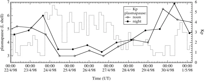
The local time asymmetry of the plasmapause is an im-portant issue. It is not easy to solve this problem, as it re-quires simultaneous observations on both sides of the Earth, or very stationary conditions. At the noon-midnight merid-ian the asymmetry is expected to be quite weak. However, in Fig. 6, the dayside and nightside plasmapause usually appear at different L-shells (except panel 4 from top), which shows that the evolution of the plasmapause can be quite fast, as the dayside and nightside observations are collected 3–4 h apart. To investigate further the evolution of the plasmapause, we again turn to the geomagnetically variable interval on 22 April to 1 May 1998, when Polar crosses the plasma-pause near noon (11:00–12:00 MLT) and midnight (23:00– 24:00 MLT). While the density profiles are displayed in Fig. 6, Fig. 7 shows the locations of the plasmapause every 18 h over the Northern Hemisphere. The variation of the Kp
index is shown by a dotted line. The scale on the left is for the plasmapause position and the scale on the right for the Kp
index. In the beginning of the interval, the geomagnetic ac-tivity is weak, and the plasmapause stays near L = 5. On 23 April, a quiet interval occurs at 9:00–18:00 UT, during which the nightside plasmapause rapidly moves anti-earthward; the dayside evolution cannot be evaluated due to a lack of mea-surements. A magnetic storm on 23–27 April is preceeded by an SSC on 23 April, 18:25 UT. The dayside plasmapause is crossed 30 min later, and it seems plausible that the plasma-pause has already moved at least 0.5 L earthward. Notice that we do not know the distance of the dayside plasmapause at the end of the quiet interval, but it is very likely that it was at least near the same distance where it was during the previous measurement due to the quiet period of 23 April.
During the storm on 24–25 April, the plasmapause appears near L = 3. For the declining phase of magnetic activity, the plasmapause moves outward from the Earth both in the noon and midnight sectors. 29–30 April is a particularly quiet period, during which the plasmasphere expands rapidly. A fast earthward movement of the plasmapause occurs after an SSC onset at 09:28 UT on 30 April 1998. Polar crosses the dayside plasmapause three hours after the onset and by then
7 6 5 4 3 plasmapause (L shell) 00:00 22/4/98 00:00 23/4/98 00:00 24/4/98 00:00 25/4/98 00:00 26/4/98 00:00 27/4/98 00:00 28/4/98 00:00 29/4/98 00:00 30/4/98 00:00 1/5/98 Time (UT) 6 5 4 3 2 1 0 Kp Kp plasmapause: noon night
Fig. 7. Locations of the plasmapause near noon and midnight on 22–30 April 1998; the L-shell scale from 3 to 7 is given on the left axis.
The panel also presents the variation of the 3-h global Kpindex, shown by a dashed line, with a scale on the right axis.
this boundary has retreated earthward by at least one L-shell. Once more, we do not know the plasmapause distance just before the onset, but again the preceeding quiet period has likely kept the plasmapause at the same position as during the previous crossing or preferably has moved it away from the Earth. Thus, we speculate that the plasmapause may be reacting quite rapidly to the changes in the convection elec-tric fields. As a result, the location of the noon and midnight plasmapause keeps changing places in the last four panels of Fig. 6.
We emphasize that these measurements are made at the noon-midnight meridian, and the evolution can be signifi-cantly different at other local time sectors, especially in the dusk sector (see, e.g. Moldwin et al., 1994; Eplhic et al., 1996). We will discuss our findings further in Sect. 3.3.
2.5 Auroral oval
The auroral zone is one of the most tenuous regions within the magnetosphere. Particularly low densities can be ob-served in auroral cavities (Persoon et al., 1988; Makela et al., 1998). Persoon et al. (1988) found clear evidence that au-roral cavitation is a result of auau-roral acceleration processes, and according to Makela et al. (1998), there is no correlation between the occurrence of cavities and geomagnetic activity. On the nightside Polar crosses the auroral zone over the Southern and Northern Hemispheres with a separation of about 2–3 h. A major difference between the observations from the two hemispheres is the observation distance, which is in the range of 3.5–5.5 RE for the Northern Hemisphere
and about 1.9 RE for the Southern Hemisphere. Due to the
compressed time scale in Fig. 2, density variations above the auroral oval are not clear, except that enhanced disturbances with some density cavities occur.
We continue our analysis by examining seven consecutive auroral oval crossings on 25–30 April 1998, which is an in-terval of highly variable activity. Figures 8a and b present
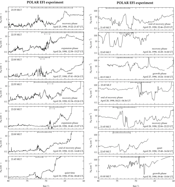
the density profiles against invariant latitude: Fig. 8a is for the Northern Hemisphere, and Fig. 8b is for the Southern Hemisphere. Notice that the density scales are different for these figures. The magnetic local time of the observations is given in each panel. Using a preliminary global AE in-dex, we have defined the level of global magnetic activity for each crossing, as indicated in the panels. These examples present density profiles collected during all substorm phases and during very quiet periods.
Although the northern and southern oval crossings are sep-arated by a few hours, in some panels one can distinguish similar features between the two profiles. On the other hand, the measurements in the two adjacent panels over one hemi-sphere are separated by about 18 h. It is clearly obvious that these profiles are not correlated.
The density profiles across the auroral zone are highly variable and presumably quite low densities should be en-countered. Therefore, it is somewhat surprising that it is not always easy to distinguish the auroral cavities in Figs. 8a and b. Note, however, that the occurrence of a low density re-gion is not enough to call it a cavity, since at high latitudes such events may be caused by irregular transitions to the po-lar cap where low densities are also encountered. There-fore, we have investigated dc-electric field variations during these events, because the electric fields are usually larger and more variable in the auroral zone than in the polar cap. The locations of enhanced electric fields are marked with solid horizontal bars in the panels. These disturbances are usu-ally accompanied by magnetic field perturbations. If particu-larly strong electric fields (i.e. more than 15 mV m−1for the northern oval, and more than 45 mV m−1 for the southern oval) are detected, it is marked with dotted horizontal bars.
One can observe that clear density cavities in the auro-ral zone do not always exist. Another obvious fact is that auroral cavities and auroral electric fields do not fully over-lap: there are cavities with no electric field signatures, and
0.1 1 10 Ne (cm –3) 80 75 70 65 60 Ilat (˚) recovery phase April 25, 1998, 19:22–21:47 UT 23:35 MLT 0.1 1 10 Ne (cm –3) 80 75 70 65 60 Ilat (˚) expansion phase April 26, 1998, 12:58–15:27 UT 22:35 MLT 0.1 1 10 Ne (cm –3) 80 75 70 65 60 Ilat (˚) onset April 27, 1998, 07:41–09:26 UT 22:00 MLT 0.1 1 10 Ne (cm –3) 80 75 70 65 60 Ilat (˚) recovery phase April 28, 1998, 01:54–03:26 UT 22:55 MLT
POLAR EFI experiment
0.1 1 10 Ne (cm –3) 80 75 70 65 60 Ilat (˚) expansion phase April 28, 1998, 18:40–21:07 UT 23:20 MLT 0.1 1 10 Ne (cm –3) 80 75 70 65 60 Ilat (˚)
end of recovery phase April 29, 1998, 12:22–14:48 UT 22:00 MLT 0.1 1 10 Ne (cm –3) 80 75 70 65 60 Ilat (˚) quiet time April 30, 1998, 07:06–08:48 UT 21:45 MLT 0.1 1 10 100 Ne (cm –3) 80 75 70 65 60 Ilat (˚)
end of recovery phase April 25, 1998, 22:46–23:03 UT 21:45 MLT 0.1 1 10 100 Ne (cm –3) 80 75 70 65 60 Ilat (˚) recovery phase April 26, 1998, 16:28–16:44 UT 22:45 MLT 0.1 1 10 100 Ne (cm –3) 80 75 70 65 60 Ilat (˚) growth phase April 27, 1998, 10:24–10:44 UT 00:15 MLT 0.1 1 10 100 Ne (cm –3) 80 75 70 65 60 Ilat (˚) end of recovery phase
April 28, 1998, 04:21–04:36 UT 23:45 MLT
POLAR EFI experiment
0.1 1 10 100 Ne (cm –3) 80 75 70 65 60 Ilat (˚) recovery phase April 28, 1998, 22:06–22:23 UT 21:45 MLT 0.1 1 10 100 Ne (cm –3) 80 75 70 65 60 Ilat (˚) quiet April 29, 1998, 15:48–16:04 UT 22:45 MLT 0.1 1 10 100 Ne (cm –3) 80 75 70 65 60 Ilat (˚) growth phase April 30, 1998, 09:46–10:06 UT 01:00 MLT
Fig. 8. (a) Crossings of the northern auroral zone in the pre-midnight sector on seven consecutive orbits of 25–30 April 1998. The crossings
(the UT interval is given in each panel) happened during different geomagnetic conditions, as marked in each panel. The solid horizontal bars indicate the locations of the electric field perturbations; the dashed bars show the locations of very strong electric fields, when they existed.
(b) same as (a) but for the southern auroral zone.
vice versa, there are large electric field perturbations with no clear density cavitation. This is a suprise to some extent, as the auroral electric fields tend to be anti-correlated with the level of plasma density (see, e.g. Lindqvist and Marklund, 1990). A clear case of an auroral cavity exists in the third
plot from the bottom on 28 April (see both Figs. 8a and b). In this event, Polar crosses the auroral zone very soon af-ter the onset of an isolated substorm. Two distinct cavities are observed over the Northern Hemisphere (Fig. 8a); how-ever, electric field disturbances appear only within the inner
cavity. One may wonder if the other one is due to a polar cap transition. This is not likely because two hours later, during the recovery phase of the same substorm, the same cavities are still observed, now over the southern oval (Fig. 8b), at slightly different invariant latitudes, possibly due to different MLT or of an evolution of the oval. In the next panel below, about 18 h later, Polar detects one wide cavity just after the end of the recovery phase of a moderate substorm. Two hours later, when the substorm is over, the cavity still exists above the southern oval. The bottom panel in Fig. 8a shows a deep and wide cavity during a very quite interval, some five hours after a substorm recovery phase. However, over the southern oval, no cavitation is observed, possibly due to the high alti-tude of the bottom of the cavity. In the top panels of Figs. 8a and b, one cannot easily distinguish any cavities. These ob-servations tend to suggest that the formation and existence of cavitation at the auroral zone is not a straightforward prob-lem.
3 Discussion
3.1 Motion of the cusp
According to the statistical results by Laakso et al. (2002), the cusp position is quite stationary for low Kpand tends to
move equatorward with increasing Kp (for a detailed study,
see Palmroth et al., 2001). During disturbed conditions, how-ever, the cusp disappears in the average density picture, even though the cusp is always observed in the noon sector, except for some rare cases, such as the quiet period of 10–11 May 1999, when no cusp was observed. Our conclusion is that the cusp position can change quite dramatically under geomag-netically active intervals. We now discuss evidence for this from individual cusp crossings.
We have found several cases where the cusp is apparently crossed twice; one such event is shown in Fig. 5. The ex-amination of the interplanetary magnetic fields from several spacecraft shows that these events occur simultaneously with variations of the IMF. This implies that the cusp can shift its position nearly instantly in response to an IMF variation. Another related feature is that individual cusp crossings fre-quently reveal steep density slopes at the equatorward bound-ary of the cusp. This is likely to be caused by a motion of the cusp, as the spacecraft speed is only a few km s−1. When the solar wind is stationary, the cusp crossing can be described by the spacecraft moving slowly through a stationary cusp. Figure 5 contains examples of such cases in the second, fifth and eighth panels from the top. Notice that the density de-cline is usually not steep on the poleward boundary of the cusp, because the densities in the cusp and the plasma man-tle are somewhat similar and the latter region is rather wide (Rosenbauer et al., 1975).
Berchem and Russell (1982) investigated the characteris-tics of the dayside magnetopause and found that it is in con-stant irregular motion at velocities 10–80 km s−1. Since the cusp motion is not driven by magnetosheath pressure
varia-tions but rather by reconnection at the magnetopause (Smith and Lockwood, 1996), it is likely to evolve at somewhat dif-ferent velocities. Unfortunately with only one satellite we cannot properly solve the velocity of the boundary, but it seems often to be much higher than the velocity of the ve-hicle and thus, likely of the order of 10 km s−1at high alti-tudes. Therefore, the cusp can assume a new position in less than 10 min in most cases. This suggests that an appropriate integration time of the solar wind measurements needed for studying the dynamics of the cusp is a few tens of minutes. 3.2 Density in the trough
We studied a sequence of orbits between L = 3 − 12 and found that the density between the plasmapause and the mag-netopause is higher on the dayside than on the nightside (see Fig. 6). This is particularly clear for quiet intervals, where the difference may be almost an order of magnitude, whereas during disturbed conditions, the densities tend to be roughly the same. One noticeable feature in the density profiles is that the dayside profiles do not change much (except the po-sition and slope of the plasmapause), whereas the nightside densities can develop strongly from orbit to orbit. The expla-nation for the difference is apparently due to the ionosphere which represents a source of plasma for the dayside magneto-sphere. This source is less important for the nightside mag-netosphere. During quiet periods, the difference, therefore, reflects the ionospheric plasma contribution, by yielding dif-ferent rates at noon and midnight, whereas during disturbed conditions the nightside near-Earth magnetosphere has ad-ditional sources, such as the plasmasphere via erosion pro-cesses, and the magnetotail via fast magnetospheric convec-tion that transport plasmas from the tail toward the Earth. Another possible explanation for the higher densities on the dayside is that as flux tubes convect from the nightside to-wards the dayside, they are continually fed by ionospheric outflows at a rate of around 0.5 to 20 cm−3/day (Lawrence et al., 1999).
By comparing the density profiles of Fig. 6 with the trough model of Carpenter and Anderson (1992), we found that the densities agreed within a factor of 2–5 on the dayside. On the nightside we used the model at 00:00 MLT, and again, sim-ilar differences were obtained. These differences are close to within the experimental error (factor of 2–3), but in most cases the difference appears consistently in the same direc-tion (i.e. our densities are usually lower than those of Car-penter and Anderson). One possible reason for the discrep-ancy may be that the Carpenter and Anderson model does not take into account the geomagnetic activity level, which has an impact on the trough density.
3.3 Evolution of the plasmapause
The coupling between the plasmasphere and the outer mag-netosphere is not yet well understood (Moldwin, 1997). Ero-sion and recovery of the plasmasphere are important issues that are inherently related to the global dynamics and
struc-ture of the magnetosphere. At the plasmapause, the den-sity suddenly decreases a few orders of magnitude over a relatively short distance (see, e.g. Carpenter and Anderson, 1992), nearly coinciding with the switch of the plasma drift from corotation to convection (Lyons and Williams, 1984). Naturally, the location of flow separatrix can move to a new position rapidly, when the convection electric field, driven by the solar wind, changes, whereas the plasmapause, de-fined by the steep density decline, evolves at a slower speed, depending on the time scales of the refilling and erosion pro-cesses.
We investigated a sequence of plasmapause crossings by Polar at 18-h intervals near local midnight and noon (Fig. 7). The observations suggest that the plasmasphere can evolve faster than usually assumed. On 23 April 1998, the day-side plasmapause is crossed 30 min after an SSC onset, dur-ing which the plasmapause has apparently moved earthward more than 0.5 L. Similarly after another SSC, on 30 April 1998, a speed of the same magnitude is detected. On the other hand, two quiet periods occurred during the same inter-val and they exhibited rapid expansions of the plasmasphere at about the same speed. These examples suggest that the time scales important to the evolution of the plasmasphere can be a few hours rather than 10–20 h (see, e.g. references in Gallagher et al., 1995). If the speed of the plasmapause evolution is one L-shell in 1–2 h, the plasmapause can as-sume any distance relative to the flow separatrix in less than 5 h. Once the plasmapause has assumed a new position, the refilling of the flux tubes takes a much longer time (Lawrence et al., 1999).
When interpreting Polar observations, one must bear in mind that the crossings occur at 18-h intervals, and the plasmapause location can develop significantly within such a time, which makes the interpretation difficult. Also, the evo-lution at different local time sectors can be quite different. Particularly strong evolution is observed in the bulge region (Moldwin et al., 1994; Elphic et al., 1996). For instance, El-phic et al. (1996) have found that the plasmaspheric bulge actually moves sunward after SSC onsets. Our observations at both noon and midnight indicate clearly that the plasma-pause moves earthward at these two sectors. The statistical pictures by Laakso et al. (2002) (see their Fig. 4) suggest that in the afternoon sector the average plasmapause/trough density remains unchanged for high Kp. This is possibly
due to erosion processes that cause detached plasmaspheric fragments that drift sunward in the dusk sector, keeping the average density high.
4 Summary
Differential potential (1V ) measurements from the Polar electric field instrument have been used to study electron density profiles in some specific regions of the magneto-sphere between 2–9 REgeocentric distances. This technique
provides a measure of the thermal plasma density to val-ues even below 0.1 cm−3with high time resolution (of time
scales less than 0.1 s). The statistical results are presented by Laakso et al. (2002), and the present paper displays den-sity profiles across some key plasma regions of the magneto-sphere. The major findings are:
1. The polar cap is one of the most most tenuous regions within the magnetosphere. Its equatorward boundary, however, does not appear as a steep density decline be-cause equally low densities can be detected in the auro-ral zone. The polar cap density data show clear asym-metry with MLT. In summer at low altitudes, the polar cap density is quite high in the central polar cap, that is, of the same order of magnitude as at lower latitudes, while this is not observed in winter or at high altitudes. 2. The cusp properties, such as the electron density and the location, change significantly from orbit to orbit. A typical density is between 40 and 100 cm−3 in the high-altitude (4–8 RE) cusp. Based on individual cusp
crossings, we found several cases where the cusp can as-sume a new position, responding almost instantaneously to changes in the IMF orientation.
3. The plasmapause location is strongly correlated with the Kpindex so that its asymmetry in MLT increases with
Kp. The strongest evolution in the plasmapause
posi-tion appears on the nightside. In two cases, after SSC onsets, the plasmapause at noon and midnight was ob-served to retreat earthward approximately in one L-shell per hour. Similarly, for quiet periods, the plasmapause was found to expand at the same speed. This suggests that the time scales for the earthward and anti-earthward motion of the plasmapause are only a few hours. For the studies of the plasmapause position, it is, therefore, enough to consider the geomagnetic activity during the preceeding 4–6 h.
4. The plasma density is clearly higher in the dayside trough than in the nightside trough, particularly during quiet intervals. On the dayside the density is usually a few electrons per cm3, whereas on the nightside it is 0.1–1 cm−3, where the low values are for low Kp and
the high values for high Kp. The difference is likely
set by the ionosphere which provides higher refilling rates on the dayside. For disturbed conditions, the night-side trough can be filled with particles from additional sources, such as the plasmasphere (detached material) and the magnetotail (fast transport due to strong con-vection).
5. The auroral zone is characterized by a highly variable plasma density with a mixture of density cavities, at various scale sizes, not always connected to regions of (large) auroral electric fields or to the geomagnetic ac-tivity level. Cavities are observed but their locations, strengths, and sizes can vary. Some of them can last for more than two hours, enabling them to be observed by Polar over both hemispheres. Electric field perturba-tions do not necessarily correlate with the cavities: there
are cavities with no electric field disturbances, and vice versa, auroral electric fields are observed with no clear cavitation. Furthermore, the occurrence of auroral cav-ities either at low or high altitudes does not correlate in any simple way with geomagnetic activity.
Acknowledgements. This work is supported under NASA grant
NAG5-3182.
Topical Editor G. Chanteur thanks G. Marklund and V. Pierrard for their help in evaluating this paper.
References
Berchem, J. and Russell, C. T.: The thickness and velocity of the magnetopause current layer: ISEE 1 and 2 observations, J. Geo-phys. Res., 87, 2108–2114, 1982.
Carpenter, D. L. and Anderson, R. R.: An ISEE/Whistler model of equatorial electron density in the magnetosphere, J. Geophys. Res., 97, 1097–1108, 1992.
Elphic, R. C., Weiss, L. A., Thomsen, M. F., McComas, D. J., and Moldwin, M. B.: Evolution of plasmaspheric ions at geosyn-chronous orbit during times of high geomagnetic activity, Geo-phys. Res. Lett., 23, 2189–2191, 1996.
Gallagher, D. L., Craven, P. D., Comfort, R. H., and Moore, T. E.: On the azimuthal variation of core plasma in the equatorial mag-netosphere, J. Geophys. Res., 100, 23 597–23 605, 1995. Gallagher, D. L., Craven, P. D., and Comfort, R. H.: A simple model
of magnetospheric trough total density, J. Geophys. Res., 103, 9293–9297, 1998.
Gallagher, D. L., Craven, P. D., and Comfort, R. H.: Global core plasma model, J. Geophys. Res., 105, 18 819–18 833, 2000. Higel, B. and Lei, W.: Electron density and plasmapause
charac-teristics at 6.6 RE: a statistical study of the GEOS 2 relaxation
sounder data, J. Geophys. Res., 89, 1583–1601, 1984.
Laakso, H. and Jarva, M.: Position and motion of the plasmapause, J. Atmos. Terr. Sol. Phys., 63, 1171–1178, 2001.
Laakso, H., Pfaff, R., and Janhunen, P.: Polar observations of elec-tron density distribution in the Earths magnetosphere. 1. Statisti-cal results, Ann. Geophysicae, this issue, 2002.
Lawrence, D. J., Thomsen, M. F., Borovsky, J. E., and McComas, D. J.: Measurements of early and late time plasmasphere refilling as observed from geosynchronous orbit, J. Geophys. Res., 104,
14 691–14 704, 1999.
Lemaire, J. F. and Gringauz, K. I.: The Earth’s Plasmasphere, Cam-bridge Univ. Press, CamCam-bridge, 1998.
Lindqvist, P.-A. and Marklund, G. T.: A statistical study of high-altitude electric fields measured on the Viking satellite, J. Geo-phys. Res., 95, 5867–5876, 1990.
Lyons L. R. and Williams, D. J.: Quantitative Aspects of Magneto-spheric Physics, D. Reidel, Dordrecht, 1984.
Marklund, G. T., Blomberg, L. G., Falthamma, C.-G., Erlandson, R. E., and Potemra, T. A.: Signatures of the high-altitude polar cusp and dayside auroral regions as seen by the Viking electric field experiment, J. Geophys. Res., 95, 5767–5780, 1990. Makela, J. S., Malkki, A., Koskinen, H., Boehm, M., Holback,
B., and Eliasson, L.: Observations of mesoscale auroral plasma cavity crossings with the Freja satellite, J. Geophys. Res., 103, 9391–9404, 1998.
Moldwin, M. B.: Outer plasmaspheric plasma properties: what we know from satellite data, Space Sci. Rev., 80, 181–198, 1997. Moldwin, M. B., Thomsen, M. F., Bame, S. J., McComas, D. J., and
Moore, K. R.: An examination of the structure and dynamics of the outer plasmasphere using multiple geosynchronous satellites, J. Geophys. Res., 99, 11 475–11 481, 1994.
Newell, P. T. and Meng, C.-I.: Mapping the dayside ionosphere to the magnetosphere according to particle precipitation character-istics, Geophys. Res. Lett., 19, 609–612, 1992.
Palmroth, M., Laakso, H., and Pulkkinen, T.: Location of high-altitude cusp during steady solar wind conditions, J. Geophys. Res., 106, 21 109–21 122, 2001.
Park, C. G., Carpenter, D. L., and Wiggin, D. B.: Electron density in the plasmasphere: Whistler data on solar cycle, annual, and diurnal variations, J. Geophys. Res., 83, 3137, 1978.
Persoon, A. M., Gurnett, D. A., and Shawhan, S. D.: Polar cap elec-tron densities from DE 1 plasma wave observations, J. Geophys. Res., 88, 10 123–10 136, 1983.
Persoon, A. M., Gurnett, D. A., Peterson, W. K., Waite, Jr., J. H., Burch, J. L., and Green, J. L.: Electron density depletions in the nightside auroral zone, J. Geophys. Res., 93, 1871–1895, 1988. Rosenbauer, H., Gr˝unwaldt, H., Montgomery, M. D., Paschmann,
G., and Sckopke, N.: Heos 2 observations in the distant polar magnetosphere: the plasma mantle, J. Geophys. Res., 80, 2723– 2737, 1975.
Smith, M. F. and Lockwood, M.: Earth’s magnetospheric cusps, Rev. Geophys., 34, 233–260, 1996.