A doubly-fed machine for propulsion applications

(1)

A Doubly-Fed Machine for Propulsion

Applications

by

Michael S. Tomovich

B.S. Electrical and Computer Engineering

ARWHNE*S

jMASSACHU$L I NST lJE OF TECHN~OLOGY

APR i o 2014

LIBRARIES

Carnegie Mellon University, 2011

Submitted to the Department of Electrical Engineering and Computer

Science in partial fulfillment of the requirements for the degree of

Master of Science in Electrical Engineering and Computer Science

at the

MASSACHUSETTS INSTITUTE OF TECHNOLOGY

February 2014

@

Massachusetts Institute of Technology 2014. All rights reserved.

A uthor ...

...

Department of Electrical Engineering and Computer Science

December 18, 2013

Certified by ..

...

Steven B. Leeb

Professor of Electrical and Mechanical Engineering

Thesis Supervisor

Certified by...

...

Arijit Banerjee

Doctoral Candidate

Thesis Supervisor

Certified by.

c__.

Arthur Chang

Doctoral Candidate

Thesis Supervisor

Accepted by. .. .

Chairman,

Leslie A. Kolodziejski

Department Committee on Graduate Theses

(2)

(3)

A Doubly-Fed Machine for Propulsion Applications

by

Michael S. Tomovich

B.S. Electrical and Computer Engineering

Carnegie Mellon University, 2011

Submitted to the Department of Electrical Engineering and Computer Science on January 21, 2014, in partial fulfillment of the

requirements for the degree of

Master of Science in Electrical Engineering and Computer Science

Abstract

A doubly fed machine for propulsion applications is proposed, which, given the

pres-ence of AC and DC power sources, can be utilized in order to improve efficiency, weight, volume, and sizing of the rotor power electronics. In this case, a shipboard application is examined. A hardware demonstration of a control architecture is im-plemented, along with a benchtop demonstration of the replacement of standard slip rings in the machine with a contactless solution (i.e. a transformer).

Along with the benchtop demonstration of the transformer for accessing the ro-tor terminals, an analysis of the power handling capability of different converters for rectifying the power from the transformer for use with the electric machine is per-formed. A half bridge, full bridge, asymmetrical PWM half bridge, and asymmetrical PWM full bridge converter are all examined in terms of feasibility and power han-dling capability in simulation. A comparison of the modeled power transfer capability and the actual power handling capability of a half and a full bridge converter is also presented.

Thesis Supervisor: Steven B. Leeb

Title: Professor of Electrical and Mechanical Engineering Thesis Supervisor: Arijit Banerjee

Title: Doctoral Candidate

Thesis Supervisor: Arthur Chang Title: Doctoral Candidate

(4)

(5)

Acknowledgments

First, I'd like to thank my parents Steve and Darla Tomovich and brother Andy Tomovich for their constant support during this and all of my endeavors. I would also like to express my gratitude to my research advisor Professor Steven Leeb for his mentorship, advice, and technical guidance.

I'd like to thank the members of MIT's Laboratory for Electromagnetic and Elec-tronic Systems who have been instrumental from both a technical and a work environ-ment perspective in helping me complete this thesis. I'd like to thank Arijit Banerjee for his wizardry of electric machines, Arthur Chang for his technical intuition and guidance, Sabino Pietrangelo for his thesis template and classroom assistance, Deron Jackson for the groundwork that he laid, and Matt Angle for his constant technical presence and friendship. I would also like to acknowledge and thank Professor Jim Kirtley for his role in my knowledge of electric machines and his technical advising.

Lastly, I'd like to thank my friends, especially Emily Creedon, Michael Street, Anton Hunt, Sabino Pietrangelo, and the Brothers of AXA for their constant support, social interaction, and adventures even throughout the most trying of times. I would also like to thank David and the Brothers of BOH at Carnegie Mellon for their continued friendship and memorable experiences.

This research was performed with support from the Electric Ship Research and Development Consortium under The Office of Naval Research. This work was also in part supported by The Grainger Foundation.

(6)

(7)

List of Figures

1-1 Multi-bus DC Power Distribution [1] ... 19

1-2 Basic Rotary Transformer [12] . . . . 22

2-1 Normalized Propulsion Power [1] . . . . 26

2-2 DFM Steady State Circuit Model [1] ... 28

2-3 DFM for Propulsion [1] . . . . 30

2-4 Normalized DFM Rotor Power (unity on the vertical and horizontal axes correspond to maximum power P, and speed Q,) [1] . . . . 33

2-5 Normalized DFM Stator Power (unity on the vertical and horizontal axes correspond to maximum power P and speed Q,) [1] . . . . 34

2-6 Electric Machine Representation in Space Vector Form [2] . . . . 35

2-7 Power Circuit of the Proposed Scheme [2] . . . . 36

2-8 Structure of q-axis Controller with Feed-forward Terms [2] . . . . 43

2-9 Structure of d-axis Current Controller with Feed-forward Terms [2] . . 44

2-10 Structure of Speed Controller [2] . . . . 45

2-11 Structure of Flux Controller during DC Mode [2] . . . . 46

2-12 Complete Controller for DC Mode [2] . . . . 46

2-13 Structure of Reactive Power Controller during AC Mode [2] . . . . 48

2-14 Complete Controller for AC Mode [2] . . . . 48

2-15 Space Vector Diagram for Determining the Correct Switching Instant for Transitioning from DC to AC [2] . . . . 49

2-16 Space Vector Diagram for Determining the Correct Switching Instant for Transitioning from AC to DC [2] . . . . 50

(12)

2-17 Signal Flow Diagram for Synchronizer [2] ...

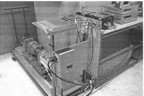
2-18 Texas Instruments High Voltage Motor Control and PFC Developers Kit 2-19 Motor Control Experimental Setup . . . .

2-20 : Experimental Results: (a) Actual speed with a commanded speed of 540 rpm (b) Estimated stator flux magnitude and electromagnetic torque without RPC or SFTC (c) Estimated stator flux magnitude and electromagnetic torque with RPC and without SFTC (d) Estimated stator flux magnitude and electromagnetic torque with RPC and SFTC (e) Stator A phase and Rotor A phase current with RPC and SFTC during acceleration (f) A phase voltage and current at 540 rpm with RPC and SFTC enabled [2] . . . . 2-21 Reference tracking of speed controller in three speed ranges - (a) DC

Mode only (b) DC and AC modes (c) AC mode only [2] . . . . T107 'Pot Core' with slot cut out . . . . Cross Sectional View of Transformer Cores Face to Face showing Flux P aths . . . .

Close-Up of Flux Path in the Inductive Coupling Reluctance Model for the Inductive Coupling . . Flux Path Lengths for Determining Reluctance Coupling Reluctance Model . . . . Areas for Calculating Ri and R . . . . Areas for Calculating Rb . . . . Dimensioned T107 Core for Sample Calculations Simplified Reluctance Model ...

Measuring Leakage Inductance ...

Measuring Leakage + Magnetizing Inductance .

3 Phase Inductive Coupling . . . .

Values in Inductive

(dimensions in mm)

DC-DC Converter with Separable Inductive Coupling . . . .

Inverter and Transformer Simplifications [22] . . . . 51 52 53 55 56 58 59 60 60 61 61 62 62 63 64 65 65 72 74 3-1 3-2 3-3 3-4 3-5 3-6 3-7 3-8 3-9 3-10 3-11 3-12 4-1 4-2

(13)

4-3 Half Bridge Rectifier Reflected to Secondary Side . . . . 76

4-4 Half Bridge Rectifier Current Modes. Left: Mode 1. Right: Mode 2. . 76 4-5 Half Bridge Rectifier in Mode 1 with -V, applied . . . . 78

4-6 Simplified Schematic for Finding I,1 . . . . 78

4-7 Simplified Converter Schematic for finding Ii with Branch Voltages Folded into Branch Sources . . . . 79

4-8 Simplified Converter with the Parallel Branches Combined . . . . 80

4-9 Simplified Converter with Simplified Voltage Source . . . . 80

4-10 Circuit Model for Determining V . . . .. 82

4-11 Close-Up of Mode 2 Current Waveform . . . . 84

4-12 Half Bridge Rectifier in Mode 2 with -V, applied . . . . 85

4-13 Mode 2 Simplified Circuit Model . . . . 85

4-14 Collapsed Circuit Model for Mode 2 Fast Ring Start Current . . . . . 86

4-15 Mode 2 i,(t) Broken into Parts . . . . 89

4-16 Half Bridge Converter Capability Plot. Vbat = 250V . . . . 91

4-17 Symmetric Full Bridge Converter . . . . 92

4-18 Symmetric Full Bridge Converter with Constant Output Voltage . . . 93

4-19 Symmetric Full Bridge Converter Current Modes. Left: Mode 1. Right: M ode 2. . . . . 93

4-20 Symmetric Full Bridge Converter Simplified Circuit Model . . . . 94

4-21 Splitting V and folding the split voltage sources into the capacitor branches. Note that all voltages across the top and bottom nodes rem ain the sam e. . . . . 95

4-22 Circuit Model (without source) that follows from folding the source voltage into the capacitor voltages . . . . 96

4-23 Simplified full bridge circuit model for finding I,1. . . . . 97

4-24 Folding Vcc into V(t) . . . . 97

4-25 Full Bridge Converter Schematic for Finding Inductor Voltage . . . . . 98

4-26 Mode 2 Full Bridge Circuit model before transition to +V . . . . . 100

(14)

4-28 Mode 2 Full Bridge Circuit Model that follows from folding the output

voltage source into the capacitor voltages . . . . 101

4-29 Mode 2 Full Bridge Simplified Circuit for Finding s2 . . . . 102

4-30 Mode 2 iZ(t) Broken into Parts . . . . 105

4-31 Full Bridge Converter Capability Plot. Vbt = 250V . . . . 107

4-32 Source Voltage for Asymmetrical PWM Full Bridge Converter . . . . . 108

4-33 Asymmetrical Full Bridge Converter . . . . 109

4-34 Asymmetrical Full Bridge Rectifier Current Modes (Left: Mode 1, Right: M ode 2) . . . . 109

4-35 Asymmetrical Full Bridge Rectifier Current Geometric Breakdown . . 113

4-36 Asymmetrical Full Bridge Rectifier Capability Plot . . . . 115

4-37 Asymmetrical Full Bridge Rectifier Capability Plot. The peak line in terms of power corresponds to a duty ratio of D = .5. . . . . 115

4-38 3 Phase Converter with Parasitics Schematic . . . . 116

4-39 3 Phase Converter Capability Plot, Vbt = 300V . . . . 117

4-40 Full Bridge Converter Schematic . . . . 118

4-41 Half Bridge Converter Schematic . . . 118

4-42 Full and Half Bridge Converter Experimental Setup. Left: H-Bridge Middle: Full Bridge Converter Right: Half Bridge Converter . . . 119

4-43 TI Motor Control Riser Card for Controlling H-Bridge . . . . 120

4-44 Experimental Data vs Predicted Capability Plot for Half Bridge Con-verter... ... 121

4-45 Experimental Data vs Predicted Capability Plot for Full Bridge Con-verter... ... 121

(15)

List of Tables

2.1 Machine Model Equations ... 40

3.1 Magnetic Core Parameters . . . . 62

3.2 A, Calculation and Dependency on Gap Size . . . . 63

4.1 Inductive Coupling Parameters . . . . 119

(16)

(17)

Chapter 1 Introduction

1.1 Background

This thesis examines the practicality and the implementation of a variable speed electric drive which takes advantage of a power system with both AC and DC supply available. That is, if a doubly fed machine is used as the prime mover, both the AC and DC elements of the power system can be utilized in order to improve efficiency, weight, volume, and sizing of the rotor power electronics [1].

The Doubly-Fed Machine (DFM) has two modes of operation. In the first mode of operation, the DC source is used on the DFM stator, and the rotor is driven with a power electronics drive. The DC on the stator makes the machine behave like a permanent magnet machine (or a synchronous motor). The DFM is operated in this mode until the shaft speed reaches the synchronous speed, at which point the stator supply is switched from DC to AC. The AC on the stator enables the power electronics drive on the rotor to accelerate the shaft past synchronous speed. In this mode, the machine behaves like a doubly fed induction machine. Additionally, reactive power can be controlled in AC mode, which gives added flexibility in system design.

In order to successfully implement such a scheme, great care must be taken in order for the transition from DC to AC on the stator to be 'bumpless' and minimize transient effects on the system. Namely, a synchronizer is essential to determine the correct instant of switching in order to minimize the transients on torque and

(18)

speed. Starting with basic motor equations, a complete control scheme is devised that uses the stator flux reference frame. Stator flux estimation is critical when using this approach. It is challenging to do this estimation in DC mode due to offsets.

A novel hybrid flux estimator was implemented in order to overcome these offsets.

This control scheme was then verified using MATLAB SIMULINK simulations by my colleague Arijit Banerjee [2], where the controller was tuned to enable bumpless control of the DFM.

The DFM currently employed in this control algorithm uses slip rings to transfer power to the rotor. While using slip rings or brushes is currently common practice in a DFM, the mechanical contact between moving slip rings and static brushes wears these components down and results in additional maintenance over the lifetime of the machine [3].

1.2 Motivation

1.2.1 Naval Power Systems

Reference [4] describes the Medium Voltage DC (MVDC)architecture at a high level, leaving great flexibility for design and customization. Studies or analyses of hypo-thetical MVDC systems for shipboard application have focused on specific aspects of systems that could become practical MVDC systems [1]. For example, in [5] and [6], the authors examine a two-bus architecture, essentially a port-and-starboard-oriented, split-plant operation of a shipboard power system. A schematic fragment generally illustrating this arrangement is shown in Figure 1-1 [1]. To create a DC power sys-tem, two AC rotating machines are employed in Figure 1-1. The electrical output

of each of these machines is rectified and used to energize one of the two DC busses shown in Figure 1-1, either "DC Bus 1" or "DC Bus 2". Resistors "R" and inductors "L" represent parasitic line impedances. Power is distributed to ship loads through "Bus Selectors" that choose which bus energizes each load. Loads can draw power from either bus, but not both at the same time. In Figure 1-1, the "Bus Selector" is

(19)

illustrated with diode "ORing," but other, potentially better performing alternatives are discussed in [5]. DC Bus I PC Source t c ,( . AC to DC Rectifier s _ous b Selector Selector (R aciFan, P..p, Propulsion... AC Source 2r LT ---- / LOA _I DC Bus 2 AC to DC Rectifier

Figure 1-1: Multi-bus DC Power Distribution [1]

In a vision where all of the distributed power on the ship is DC (DC Bus 1 and Bus 2 in Figure 1-1), essentially all loads interface to the power system through a power electronic interface. DC-DC converters transform voltage and current levels for electronic loads like radar, computers, and potentially some weapon systems. DC-AC converters create alternating voltage drives for loads like motors employed as pumps, fans, and likely the largest of all electrical loads on the ship the electric propulsion drive. In this vision, the AC-to-DC rectifiers, which interface the AC sources to the

DC busses, must transform essentially all of the available AC power to DC, including

all of the power for the ship propulsion drive.

This approach by the schematic fragment in Figure 1-1, is anticipated to provide a number of benefits. Many of these are discussed in [4]. Some of these anticipated benefits include:

9 Efficiency: Total conversion of all AC generated power to DC decouples the

speed of the prime mover from the bus frequency. A gas turbine prime mover, for example, could be freed from operating at a fixed speed to maintain an AC bus frequency. Instead, the gas turbine speed could be adjusted to the power demand, improving fuel consumption.

e Weight and volume: The DC-DC converter shown in Figure 1-1 represents a

(20)

cur-rent level to new output DC levels appropriate for the load. These converters can operated at relatively high frequency 100s of kilohertz or more and there-fore employ lighter, smaller inductors, capacitors, and transformers compared to 60 Hz or similar frequency systems.

" Improved acoustic signature: In principle, without a common operating

fre-quency, e.g., 60 Hz, the acoustic signature of the overall ship machine plant has a broader signature that would prove more difficult to identify and track.

" Uninterruptible or fight-through power: the multi-bus arrangement with a

suit-able bus selector can provide continuous power to loads even in the face of significant damage or casualty on one of the DC busses. In principle, a bus casualty on one side of the ship would cause loads to draw power from the re-maining working bus through the bus selector. Only a catastrophic failure of

all generation could interrupt power to the loads.

The general power system architecture suggested by the notional fragment in Figure 1-1 is potentially reasonable if propulsion power is provided by a variable speed electric drive, and if the entire electric propulsion power must be provided by a

DC bus energizing the variable speed, DC-AC inverter for the propulsion motor. The

propulsion motor is likely the largest electrical power consumer on this hypothetical ship. In this case, since most of the generated power must be made available as DC power for the propulsion drive, it is probably reasonable to convert all of the power on the ship to DC, providing both propulsion power and the additional power necessary to run radar, electric weapons, and all of the other loads on the ship. The perceived benefits of MVDC distribution are concomitant with the assumption that full DC propulsion power must be available and might as well be distributed everywhere on the ship. The mechanical prime mover could, in this case, turn at variable speeds and achieve associated fuel economies, as well as moving operating acoustic signature off of a fixed frequency. Weight and volume could be saved by employing high frequency switching power converters on the DC side of the distribution system, and, with the right bus selectors, a degree of uninterruptible power may be achieved.

(21)

It may be possible to radically improve fuel economy without DC power distri-bution. It may also be possible to create a variable-speed electric propulsion drive with significantly reduced requirements for DC power. If so, an alternate MVADC architecture could provide many of the sought benefits while eliminating architectural choke-points that could limit the robustness of the ship power system.

1.2.2 Rotary Transformer Applications

In todays world, the most common way to access the rotor of any type of rotating machinery is by using brushes and slip rings. However, the mechanical contact as-sociated with brushes and slip rings wears these components down, which decreases their overall lifetime and increases maintenance costs over the lifespan of the ma-chine. When looking at developing a rotary transformer, it is useful to do so in the context of its potential uses. There are many traditional applications of traditional electric machinery for a doubly fed machine, such as in wind turbines or flywheel en-ergy storage [7] [8]. Other applications could include transferring power to helicopter blades for deicing, using an electric machine in an explosive or sealed environment where physical separation between the load/machine and the source is unavoidable or cleanliness is paramount [9]. Other rotary transformer applications are discussed in [10].

While a doubly fed machine may not be the most popular machine in use, it represents the most general case. That is, a doubly fed machine can be run as an induction machine by powering the stator and shorting the rotor, and also represents the worst case scenario in terms of power electronics for driving the rotary transformer are concerned. To be more specific, in a propulsion system such as in [2], there is a scenario where the rotor will regenerate power into its power electronic converter, thus requiring that this converter be bi-directional.

There has been some previous work performed in the area of wireless power trans-fer to replace brushes and slip rings, beginning in the 1970s for spacecraft applica-tions [11]. A rotary transformer solves the mechanical contact problems associated with brushes and slip rings, but adds other interesting design complexity and degrees

(22)

of freedom.

Wireless power transfer in a rotary transformer is typically accomplished via an inductive coupling. That is, a rotary transformer is similar to a traditional closed core transformer, only in this case, one half of the transformer is rotating. The system is still inductively coupled, only the 'rotor' (secondary) side of the transformer is spinning along with the rotor of the machine, and an air gap exists between the stator and rotor.

A rotary transformer requires power to be sent across the air gap at high frequency

(100kHz) in order to be efficient. Given that the supply will likely be a DC bus, this requires some power electronics, most likely an H-bridge or an inverter. However, a DFM for propulsion applications already needs a power electronics converter on the rotor side, so there is no additional cost incurred there. In some stages of this research, a Texas Instruments High Voltage Motor Control & PFC Developers Kit was used to drive the primary side of the transformer.

Fro]

Rotor

Stator

Figure 1-2: Basic Rotary Transformer [12]

While there is some room for design choices to be made in regards to the exact geometry of the inductive coupling, the logical approach is to employ an axial flux design. In the case of [11] and [13], the rotor and stator windings of the inductive coupling are concentric, as shown in Figure 1-2.

(23)

1.3 Thesis Organization

This thesis begins with a general description of variable speed electric drives (VSDs) and a doubly-fed machine (DFM) for propulsion applications in Chapter 2. A deriva-tion and explanaderiva-tion of a control scheme for a DFM for propulsion applicaderiva-tions that uses underrated power electronics is also presented in Chapter 2. Following a re-view of magnetic reluctance models, Chapter 3 presents a method for modeling and designing an inductive coupling for a rotary transformer to have a predictable induc-tance, as well as a comparison of material savings in a three phase vs a single phase transformer for a rotary transformer application.

A derivation and presentation of a power handling capability analysis for several

types of power converter/inductive coupling systems is presented in Chapter 4. This chapter can serve as a guide for designing and selecting an inductive coupling for an application given a voltage and power operating point.

Lastly, this thesis is summarized in Chapter 5. Applications of the presented control architecture and extensions of the existing hardware to more a practical DFM system are discussed. Future work for completing these goals is also presented.

(24)

(25)

Chapter 2 Variable Speed Electric Drive

2.1 Shipboard Application

The propulsion power required by a displacement-style hull grows rapidly with speed

[1]. The torque required to turn a propeller is generally a nonlinear function that

increases with speed. A model of required shaft torque as a function of shaft speed might, for sake of discussion, be modeled with a square-law dependence:

T = #q2 (2.1)

where

#

is a constant related to the effective viscosity or "resistance" seen by the propeller in seawater. Shaft power Pm is the product of shaft torque and shaft speed:

P, = TQ =#Q 3 (2.2)

For any particular ship design, there will be a design-maximum shaft power P as-sociated with a maximum shaft speed . At any speed, we find "Observation 1": the ratio of shaft power to the cube of shaft speed might be modeled as constant:

PM PO

P = (2.3)

FtQ3 _Q3

(26)

That is, maximum power P and speed Q, are each indicated on the graph at unity on the vertical and horizontal axes, respectively.

It is possible to exploit the rapid growth of shaft power with speed to construct a variable drive that draws the bulk of its power from a fixed frequency AC source at high speeds. The argument that follows is applicable to any situation where shaft power grows monotonically with speed; that is, the choice of a cubic model relating shaft power and speed is for illustration, although this is likely to be a reasonably representative model. 01 / 0.9 --- --- ---- ---0.4 --- --- --- --- --- --- --- ---E 0.2 --- A --- --- --- A--- --- --- :L---E t O .6 -- - --- - -Z 0 .5 -- - --- -- I 03 CL 0. 1 --- --- - --- --- --- - ---0 0 0-1 0-2 0.3 0.4 0.5 0.6 07 0.8 0 9 1

Shaft speed, fraction of maximum

Figure 2-1: Normalized Propulsion Power [1]

2.2 Doubly-Fed Machine

The proposed drive employs a wound rotor induction machine as the propulsion mo-tor, sometimes called a doubly-fed machine or DFM here. This type of machine is used in electric power generating windmills [14]. The DFM has windings on both the stator and the rotor. Electrical contact to the rotor windings is made through a set of slip rings. The stator and rotor windings can be operated shorted, or energized with DC current, or driven with a fixed or variable frequency AC source. Several

(27)

dif-ferent combinations of winding excitation produce a useful motor. For example, with the rotor windings shorted and the stator driven with a fixed frequency AC source, the DFM operates in a manner essentially identical to a conventional squirrel-cage induction machine.

2.2.1 Steady State DFM Model

Figure 2-2 shows the "steady-state" circuit model of the DFM, which can be useful for understanding the operation of the machine [1]. The machine is essentially similar to a transformer, with primary windings on the stator and secondary windings on the rotor. The circuit model in Figure 2-2 is similar to the conventional "T-model" used to represent a single-phase transformer or one phase of a line-neutral stator connection on a wye-wound squirrel-cage induction machine. The model components V, R₁, L1, and Lm in Figure 2-2 represent the stator applied voltage, resistance, leakage

inductance, and magnetizing inductance, respectively. The vertical line through the nodes labeled a and g is the "air-gap" line, which marks the point in the circuit model separating lumped model elements on the stator from those on the rotor. The model components L2, R, and V, represent rotor leakage inductance, resistance, and

source voltage, respectively. These components have been reflected across the "ideal transformer" that could otherwise be included in the model, and also have been scaled as appropriate by slip to account for the relative motion between the stator and the rotor. The slip s is the unitless quantity that represents the difference between the stator frequency and the shaft speed times the number of pole pairs, all divided by stator frequency. In a squirrel-cage machine, the rotor windings are shorted together, and the source V, can be replaced by a short. In the DFM, a rotor voltage V, can be applied through the slip rings. A current I is induced in the reflected rotor components to the right of the air-gap line in Figure 2-2.

(28)

R1 Li L2

R/s

Lm o

V I+

9 \

Reflected Rotor Model

(s = slip) Figure 2-2: DFM Steady State Circuit Model [1]

A key to understanding the DFM is the recognition that that reaction torque

on the stator must equal the motive torque on the rotor. This observation can be expressed quantitatively by examining the power transfer from the electrical sources driving the machine, V and V, in Figure 2-2, to the mechanical shaft. Net real power

Pa, flowing left-to-right in Figure 2-2 across the air-gap line must come from the stator

source. Power can also flow from the rotor source V, but no net real power from the rotor source contributes to Pa, any power flowing left-to-right across the air-gap line from the rotor source must first flow right-to-left across the air-gap line, for a net zero contribution crossing the air-gap line. Ignoring ohmic losses in R1 on the stator,

and a constant factor for the number of phases, and assuming that the rotor power electronics are controlled to deliver real power, the net real power delivered by the stator source is approximately equal to the net real power crossing left-to-right across the air-gap line:

R V

Ps ~ Pag = 2 -+ I 'V (2.4)

S S

The rotor inductance L2 absorbs no real or average power. Some of the real power

Pag performs electromechanical work, and the remainder is delivered to the electrical elements R and V, in the rotor circuit. The component of power P, performing electromechanical work, Pm, is the difference:

(29)

Pm =Ps I2 R -I-V,=Ps(1-s) (2.5)

The actual steady-state shaft speed of the DFM, Q, is by definition related to the synchronous shaft speed, Q, (the stator electrical frequency divided by the number of pole pairs), by the slip:

Q= QS(1 - s) (2.6)

The shaft torque is the quotient of shaft power Pm divided by shaft speed, which is now visibly identical to the real power provided by the stator source divided by the synchronous shaft speed:

Pm

-P . (2.7)

This "Observation 2" implies the equivalence of the rotor and stator reaction torques, which can be conveniently expressed as either a ratio of mechanical or elec-trical power divided by the appropriate "speed" or frequency in the associated frame.

2.3 Propulsion Drive

At least two different operating configurations of the DFM concern us here for a ship propulsion application [1]. We begin by assuming that the variable frequency power electronics associated with the rotor will only deliver power into the machine. This simplifies the analysis of the machine, and eases the requirements on the ship power system by avoiding the need to absorb regenerated power from the DFM. This assumption is not required, however, and the possibility of operating the DFM with bi-directional power electronics will be revisited shortly. The two operating configurations are illustrated schematically in Figure 2-3.

In the first operating configuration, the DFM stator is energized with DC excita-tion. In essence, the stator serves as an electromagnet, creating a fixed set of north and south magnetic poles in the fixed, non-rotating reference frame of the ship. The rotor is energized with variable frequency AC waveforms from a power electronic drive. In this configuration, the magnetic field patterns created by the stator and rotor with

(30)

power electronic drive are much like a classic, brushed, "Edison-style" wound-field

DC motor. Of course, the DFM has no mechanical commutator, only slip rings the

variable speed drive for the rotor serves as an "electronic commutator," and the ma-chine is capable of producing torque. The DC power used to energize the stator is likely to be negligible, limited to the ohmic losses on the stator. Some significant, to be minimized, DC power will be needed to energize the variable frequency power electronics associated with the rotor.

Propulsion

DC Source

Source D

Variable F

Frequency

Drive Stator Connections

Motor Rotor (Slip Ring)

Connections

Figure 2-3: DFM for Propulsion [1]

A threshold in operating condition is reached when the stator is energized with DC current and the rotor receives AC waveforms from its power electronic drive that

are at the same frequency as the synchronous or utility electric frequency, assumed fixed, on the ship. At this point, the machine could be operated in either of two configurations, either of which will produce identical torque and speed.

The DFM could be operated with DC current on the stator and AC created by the rotor power electronics at synchronous utility frequency on the rotor. Alternatively, at this synchronous shaft speed Q5, the rotor could be energized by a DC current, and the stator could be powered by the fixed-frequency AC bus that is conventionally available on most ships. This alternative configuration creates a magnetic field pattern typically associated with a "brushless" DC or permanent magnet synchronous machine. If the DFM operates with fixed-frequency AC on the stator and DC current (zero frequency)

(31)

on the rotor, it runs at synchronous speed. Rotor power drops to just the ohmic dissipation associated with running the rotor windings at DC likely a negligible amount of power.

The DFM rotor can be further accelerated in a second operating configuration, with the stator connected to the fixed frequency AC source and by energizing the

rotor with the power electronic AC drive. Rotor power, increasing from zero at synchronous shaft speed, is again delivered to the rotor from the variable frequency power electronic drive, accelerating the rotor past synchronous speed. The machine operates with negative slip. Significant power is also delivered to the machine stator from the fixed-frequency AC source.

In summary, if the goal is to minimize the total amount of DC power needed for the propulsion drive, and also to operate the power electronics strictly with electric power delivery into the DFM, avoiding the need to regenerate electric power on to the ship power system, the machine would begin operation at zero speed in the first configuration. With the stator energized by DC current, the rotor is energized by the power electronics, gradually increasing in power, electrical frequency, and shaft speed to any required operating frequency below synchronous shaft speed. At this "cutover" or synchronous shaft speed, the rotor electrical power reaches its peak, and the machine is transitioned to the second operating mode. The stator is disconnected from the DC supply, allowing enough time, likely tens of milliseconds, for the DC current to decay, and then connected to the ships utility AC supply. Once the AC supply is connected to the stator, the rotor can be excited, most likely by power electronics configured to look like an adjustable frequency current source that will inject current to push against the rotating flux wave created by the stator.

The rotor power electronics can be limited to a peak power level equal to the needed rotor power at the synchronous shaft speed. The peak shaft speed, which exceeds synchronous shaft speed, will occur in the second operating mode as the rotor accelerates past synchronous speed. The rotor electronics eventually reach peak operating power for a second time. Equating the rotor power requirement at the end of the first operating region at synchronous speed with the level at the end of the

(32)

second operating region at full shaft speed permits determination of the power rating requirements for the rotor electronics.

We write the rotor power equations for each of the two operating configurations. In the first operating configuration, the rotor power P provided by the power electronics is equal to the mechanical power Pm. Employing the previous "Observation 1," essentially all of the motive power for the DFM in "low-speed" operation comes from the rotor power electronics:

Pr = P. = PO( Q (2.8)

In the second operating configuration, the rotor power is equal to the difference of the shaft power and the real stator power, i.e., the "extra" shaft power not provided

by the stator. This equivalence can be written using both "Observation 1" and

"Observation 2":

Pr=PM-P=Po - _-) (2.9)

To determine the necessary rating of the rotor power electronics, we can equate the rotor power at synchronous shaft speed at the end of the first operating region with the rotor power at maximum shaft speed at the end of the second operating regime:

PO -Q o (2.10)

Identifying the ratio of synchronous shaft speed to maximum shaft speed as this equation can be simplified to:

S

+ - 1= 0

=

(2.11)

Solving this equation yields f, = 0.68 for practical values. For this example where

propulsion power increases as the cube of speed, the synchronous shaft speed will be located at 68% of full shaft speed, assuming rotor power electronics rated for the propulsion power required at synchronous shaft speed. Different values for

f,

will be found for speed/power relationships that are other than cubic, but this result is generally representative of what is likely.

(33)

Now, the rotor power equations can be used to plot normalized rotor power as shown in Figure 2-5 over the full shaft speed variation. For speeds below the syn-chronous shaft speed, i.e., approximately 0.68 on the horizontal scale, the DFM oper-ates in the first operating configuration. Essentially all of the shaft power is provided

by the rotor. Past this speed, the DFM operates in the second configuration, with

motive power supplied to the shaft by both the stator and rotor. The normalized stator electrical power at any operating speed, shown in Figure 2-5, is the difference between the mechanical shaft power in Figure 2-1 and the delivered rotor power in Figure 2-4 at the particular shaft speed. As indicated in Figure 2-4, the rotor power peaks at two operating speeds, the synchronous shaft speed and the peak shaft speed at unity.

For this example, the maximum required power for the rotor, and therefore the DC bus powering the rotor drive, is ideally limited to less than a third of peak propulsion power. 1. -- - -- - - - -I - - ---- -I - - - -- -- - - -I - - - - -0.8 --- --- 4--- --- -- -- -E E 0 03 1A---.4---- - 7 ---- .--02 0 0 0-1 012 0.3 04 0,5 0-6 0.7 0.8 0.9 1

Shaft speed, fraction of maximum

Figure 2-4: Normalized DFM Rotor Power (unity on the vertical and horizontal axes correspond to maximum power P and speed Q,) [1]

(34)

1. -- - - -I - - --- - -- -- -- -I - -I -- - - - - - - - - - -- -

-0

03 ----. 2- 3 4 .--

7--E

0

Shaft speed, fraction of maximum

Figure 2-5: Normalized DFM Stator Power (unity on the vertical and horizontal axes correspond to maximum power P0 and speed

&o)

[1]

If the rotor power electronics can operate reversibly, i.e., with the ability to transfer power to or from the rotor, the required peak power electronic rating can be further reduced [15]. This would therefore further reduce the amount of DC power required to energize the propulsion drive. However, the ship power system would have to be able to accept regenerated power from the rotor power electronics. This is no problem in principle, but may have implications for power quality and system stability that need further exploration.

2.4 Machine Model for Analysis

Space vector representation is a comprehensive way of representing an electrical ma-chine and its dynamics. A space vector is defined as a three phase quantity as:

= X + aX + a2_Xc

(35)

where

j2 1

v'3

a=e- = (2.13)

2 2

Xa, Xb and X, are any three phase quantities like voltages, currents, fluxes etc. and is its space vector representation. As expected, it has both real and imaginary

components (which amount to phase angle and magnitude).

We will start with basic machine equations using space vector representation. The two voltage equations are:

d

-V- = RsIs + -- 5 (2.14)

dt

Vr = RrIr + -or (2.15) dt

and the two flux equations are:

= LI,+ MIre"e (2.16)

O= Lrr + Mlse - (2.17)

while Equation 2.14 and Equation 2.16 are in the stator reference frame, Equation 2.15 and Equation 2.17 are in the rotor reference frame. This is illustrated in Figure 2-6. If a space vector is said to be with respect to the stator reference frame, it implies that it is with the respect to the stationary stator a-phase axis. For example, stator flux

L'

has an angle a with respect to the stator a-phase axis. Similarly, rotor flux

has an angle of

#

with respect to the rotor a-phase axis.

q-axis __

Rotor A

- phase axis

V 0 --- Stator Aaor

phase axis

(36)

For the sake of completeness of the machine model, the electromagnetic torque equation is:

T = -MIm

[T(Tr

ee) (2.18)

3

and the simplified mechanical model is given by

dw

J + B = r - TL (2.19)

dt

2.5 Bumpless Control of DFM with DC/AC

supply on Stator

2.5.1 Power Circuit and Choice of Reference Frame for

Control

The proposed DFM setup is connected to a DC/AC source on the stator side and a controlled inverter on the rotor side as shown in Figure 2-7. For the time being, we will assume the parameters of the DFM are well known and remain constant.

Switching

Controller Gas

DFM Constant Voltage

DC Suppy Sicng Stator Rotor

3 Phase Constant voltage constant 3 ph e frequency ACPoe Supply Converter Front End Conerter I Rectifier

Figure 2-7: Power Circuit of the Proposed Scheme [2]

(37)

flux reference frame, rotor flux reference frame, air-gap flux reference frame or stator voltage reference frame. Since we will be switching stator voltage (between AC and

DC), the stator voltage reference frame will see a transient, and will degrade bumpless

control performance. Stator flux reference frame has two main advantages over the other choices of reference frames. First, during AC mode, the stator flux is governed

by stator voltage and frequency. During DC mode of operation, stator flux is governed

by the stator current and the magnetizing component of rotor current. Thus, a

stator flux estimator is essential in order to identify the transient effects on the flux during the transistion between AC and DC mode. Second, in a conventional DFM for a wind turbine application, the stator flux reference frame allows easier control of stator reactive power, which can further benefit optimizing the inverter sizing on the rotor [16]. From a control standpoint, having the ability to measure the disturbances on the system can lead to a better a controller design and bumpless transition. Thus, the stator flux reference frame is chosen for controlling the DFM in both AC and DC mode.

2.5.2 DFM Model in Stator Flux Reference Frame

For the analysis, all the machine Equations 2.14 - 2.18 are transformed to d-q

coor-dinates, where d-axis corresponds to stator flux axis and q-axis is perpendicular to stator flux axis. Now,

-=4'_e"a (2.20)

-=(2.21)

The stator quantities can be transformed to the stator flux axis as

Vsd + JiVs = Vse-(2.22)

(38)

Similarly, all the rotor quantities can be transformed to the stator flux axis as

Vrd+

jV,,

= Ve-i(-)

Ird + jIrq =Tre-*E) (2.23)

'O-rd + IVkrq = Ore-j(ae)

where c is the angle between the stator a phase axis and the rotor a phase axis, and the rotor rotational speed is defined as

-- =

we

(2.24)

dt

With this background, first Equation 2.16 is transformed to the stator flux reference frame. This requires it to be multiplied with e-ic since it is in the stator reference frame (or stationary reference frame). This results in

= LsIe-i" + MZreiee-" (2.25) Using Equations 2.21 - 2.23, Equation 2.25 can be simplified by equating real and imaginary parts. This results in

0 =LI, + MI,, (2.26)

s= LJIsd + MIrd (2.27)

Next, Equation 2.17 is transformed to the stator flux reference frame. This requires it to be multiplied with e-i(-6) since Equation 2.17 is in the rotor reference frame. This results in

ie-j(aE)

=

LTre-(C-E) + MTS

e-E-(a-E)

(2.28) Again, this can be simplified using Equations 2.22 and 2.23 and separating real and imaginary parts.

(39)

= LIlq + M Isq

Before transforming the voltage equations into the stator flux reference frame, an identity will be derived. For any space vector X,

dX d(XejA) dt dt eA + j dAXej dt dt 1

AdX

= dX +dA dt dt dt (2.32)

Transforming Equation 2.14 to the stator flux reference frame by multiplying e-ic as before yields

dR

(2.33)

Utilizing Equations 2.22 and 2.32 and separating real and imaginary parts as before results in,

d

Vsd = R.Isd + -dt Vsq Rs Isq+@ -d (2.34) (2.35) It is worth noting that in steady state, stator supply frequency is given by,

da

di (2.36)

Similarly for Equation 2.15, multiplying it with e-i(a-) to transform it to the stator flux reference frame yields

dt

(2.37)

This can be simplified and separated into real and imaginary parts as before resulting in,

d

Vrd = RIrd + d - (Ws - rq

d

V/r = RrIrq +

drq

+ (Ws - We) Ord

(2.38)

(2.39) or

(2.31)

(40)

The torque equation can also be simplified by using Equation 2.16 in 2.18, resulting in

2M

S=3 LSt I9 (2.40)

Finally, the machine model in the stator flux reference frame using Equations 2.26, 2.27, 2.29, 2.30, 2.34, 2.35 and 2.38-2.40 is summarized in Table 2.1 below:

Table 2.1: Machine Model Equations

Differential Equations Linear Equations By Definition

d s = Vd - RsIsd Vs = RsIs +wSS -1 T

Tj Ord = Vrd - RrIrd + (Ws Werq Os LsIsd + MIrd We =d TOrq = Vq - RRIrq - (C=L -Wes) Ord 0 LsIsq + M Irq

J4 + BW = T - TL Or = LrIrd + MIsd

/rq = LrIq + MIsq

T= 2MOsIr

2.5.3 Stator Flux Estimation

Stator flux estimation is critical to orienting the measured voltage and currents along the stator flux axis for simplified control. Traditionally, stator flux is estimated either through a voltage model or through a current model in the stationary reference frame (a 3). In the voltage model of stator flux estimation, an integrator is used to compute flux along the a and 3 axes through the following equation,

d

Vsc + jVs, = Rs (Isc + jIsp) + d ("Psa + jO.s9/)

dt (2.41)

Simplifying real and imaginary parts,

sc = f (Vsa - RsIsa)dt po = f (Vo - RsIso )dt

(41)

The stator flux magnitude and angle can be computed through

0= Os 2 _(2.43)

a = tan(

It is well known that the integrator results in an estimation error due to presence of measurement offsets in the stator voltage and current. A low pass filter can be used instead of an integrator to estimate the stator flux. The cut-off frequency of this low pass filter is chosen well below the stator flux frequency. However, in this proposed method, the stator flux frequency can reach zero (in DC mode), and hence the low pass method cannot be used to estimate stator flux. A current model can also be used to estimate the stator flux using,

, = LjI + MIeie (2.44)

In this case, measurement of both stator and rotor current is essential.

A new algorithm is proposed in which the DC stator flux can be estimated while

only measuring the rotor current and stator voltage, even in the presence of offsets in these measurements. Using Equation 2.44, stator current is substituted in Equa-tion 2.14, resulting in,

-

R

S

ee

d-V=

R(bs

-M r +-S (2.45)

Ls dt

denoting the rotor current in stator flux coordinates as

Ira + JIr0 = Iese (2.46)

Separating real and imaginary parts of Equation 2.45 using Equation 2.46,

R d

VS0 = - (050 - MIr3) + -@i/so (2.47)

Ls dt

Vsa = -R(@sa - MIra) + dsc (2.48)

(42)

Rearranging,

d Rs R8M

- sa+- sa=Vsa+ Ira (2.49)

dt Ls L(

d R8 R.M

d 8+ R5 = VS + L Ir6 (2.50)

The form shown in Equation 2.49 and Equation 2.50 is inherently "low pass", which results in the best possible estimation of and in the presence of measurement offsets (unlike using the voltage model method). Furthermore, Equation 2.43 can be used to estimate stator flux magnitude and stator flux angle. The stator flux can only be estimated with stator voltage and rotor current measurements using this method. This usage of stator current measurement increases the robustness of the control algorithm. However, as seen in Equation 2.49 and Equation 2.50, this approach involves parameters of the DFM such as stator resistance and inductance, which may vary with time in a physical implementation (unlike our initial assumption in this derivation). Future work could include using stator current measurements to estimate motor parameters to enhance stator flux estimation.

2.6 DC mode: Stator Flux Oriented Control

The control loop is based on traditional inner/outer loop control where the inner loop is used to control currents and outer loop is used to control the flux and speed of the machine.

2.6.1 Design of Q-axis Current Controller

Using Equation 2.16 and Equation 2.30 in Equation 2.39 results in,

Vrq = RrIrq+ Lr -L

)

5Ir+ (ws -We)Vrd (2.51)

(s

)

dt

The controller can be designed using the above equation as shown in Figure 2-8 in order to control the q-axis rotor current using the q-axis rotor voltage.

(43)

/[I Insde

Externa

Figure 2-8: Structure of q-axis Controller with Feed-forward Terms [2]

The feed-forward term (Ws -we)Vrd is added after the PI controller output to

ensure an easier PI controller design based on the inductances and resistances as shown in Figure 2-8. Thus Kp and Ki can be chosen based on desired time constant for q-axis current control loop.

2.6.2 Design of D-axis Controller

Using Equation 2.29 in Equation 2.40 and substituting for 'Prd,

d

Vrd = Rrr + -(ILrlrd + MIsd) - (we -we) ) rq (2.52)

Substituting for Isd using Equation 2.27,

Vr = RrIrd + Lrd - M2dIrd + M

Ps

(Ws -We ) (2.53)

Ls dt Ls dt

Finally substituting Equation 2.34 for and using Equation 2.27 for Isd results in

Vr =RMIr! +)( - A Ird + '(/sd - Rs "-- - (Ws -We)krq (2.54)

This can be simplified to

(44)

Using the above equation, the d-axis current controller can be designed with three feed forward terms. Figure 2-9 shows the structure of the d-axis current controller.

M _{M V} (a). Xi > COOi (W-- V -l-' -v+ M22 R, M R'M Extera. Isd

Figure 2-9: Structure of d-axis Current Controller with Feed-forward Terms [2]

As before, Kp and Ki can be chosen based on the desired time constant for the d-axis current control loop.

2.6.3 Design of Speed Controller

The speed controller can be designed using the simplified first order mechanical model of the electrical machine. It is assumed that the q-axis current controller has signifi-cantly higher bandwidth than the speed controller (at least 10 times higher) in order for the following procedure to be valid. Typically, in electrical machines electri-cal time constants are much higher compared to mechanielectri-cal time constants. Using Equation 2.18 and Equation 2.40 and simplifying the speed control loop, Figure 2-10 can be used to design a PI controller for speed controller of a desired bandwidth.

(45)

* Inside Extemal Machine

Figure 2-10: Structure of Speed Controller [2]

2.6.4 Design of Flux Controller

In DC mode, since the stator is connected to a constant magnitude voltage source V,, the stator flux will be dependent on the load. This can be seen in Equations 2.34,

2.35, and 2.26. As the load increases, this implies the following relationship:

I,, T-> Is,

1->

V, T=> Vd 1=> Isd I=> V). I

A flux controller is essential for maintaining a constant stator flux and can be

achieved by controlling d-axis rotor current. Using Equation 2.27 in Equation 2.34, substituting in for Isd and simplifying yields:

L, d 1 -L ₈ (56

L s d I _LsVsd +Ird

'-0s + -Os= "

~+Ia(2.56)

MR5

dt

M

MR

Thus, a flux controller can be designed as before with a desired time constant and utilizing the following control loop.

(46)

Ki +

Kp+- + L3

Estimated

Inside

Extenal Machie

Figure 2-11: Structure of Flux Controller during DC Mode [2]

In DC mode, the overall control structure is shown in Figure 2-12 after combining all the controllers that have been developed so far. There are limits on the cur-rents and voltages since there will be a finite limit from both the switching converter

standpoint as well as the machine rating standpoint.

Flux controller D-axis current controller

Fei r Faedforwad

teffns tefns

Speed contruller Q-axiscurent controller V g, FtedforwBC

Figure 2-12: Complete Controller for DC Mode [2]

2.6.5 AC Mode: Stator Flux Oriented Control

When the stator is connected to an AC supply with frequency

f

8

,

-S

= --- ; fS = - (2.57)

A doubly-fed machine for propulsion applications

A Doubly-Fed Machine for Propulsion

Applications

by

Michael S. Tomovich

B.S. Electrical and Computer Engineering

ARWHNE*S

APR i o 2014

LIBRARIES

Carnegie Mellon University, 2011

Submitted to the Department of Electrical Engineering and Computer

Science in partial fulfillment of the requirements for the degree of

Master of Science in Electrical Engineering and Computer Science

at the

MASSACHUSETTS INSTITUTE OF TECHNOLOGY

February 2014

@

Massachusetts Institute of Technology 2014. All rights reserved.

A uthor ...

...

...

Department of Electrical Engineering and Computer Science

December 18, 2013

Certified by ..

...

Steven B. Leeb

Professor of Electrical and Mechanical Engineering

Thesis Supervisor

Certified by...

...

Arijit Banerjee

Doctoral Candidate

Thesis Supervisor

Certified by.

c__.

Arthur Chang

Doctoral Candidate

Thesis Supervisor

Accepted by. .. .

Chairman,

Leslie A. Kolodziejski

Department Committee on Graduate Theses

A Doubly-Fed Machine for Propulsion Applications

by

Michael S. Tomovich

B.S. Electrical and Computer Engineering

Carnegie Mellon University, 2011

Abstract

Acknowledgments

Contents

List of Figures

List of Tables

Chapter 1

Introduction

1.1

Background

1.2

Motivation

1.2.1

Naval Power Systems

1.2.2

Rotary Transformer Applications

Fro]

1.3

Thesis Organization

Chapter 2

Variable Speed Electric Drive

2.1

Shipboard Application

#

2.2

Doubly-Fed Machine

2.2.1

Steady State DFM Model

2.3

Propulsion Drive

S

=

f,

&o)