Dynamic Vehicle Routing for Robotic Networks
by
Marco Pavone
Laurea in Ingegneria Informatica, Universita degli Studi di Catania (2004)
Diploma, Scuola Superiore di Catania (2005)
Submitted to the Department of Aeronautics and Astronautics
in partial fulfillment of the requirements for the degree of
Doctor of Philosophy
at the
MASSACHUSETTS INSTITUTE OF TECHNOLOGY
June 2010
@
Massachusetts Institute of Technology 2010. All rights reserved.
ARCHIVES
Author...
...
Department of Aeronautics and Astronautics
May 26, 2010
C ertified by .... ... ...
.
...
? E
i
lio Fazzoli
Associate Professor of Aeronautics and Astronautics
Thesis Supervisor
Certified by...
Certified by...
Jonathan P. How
Professor of Aeronautics and Astronautics
' 'h Thesis Committee Member
John N. Tsitsiklis
Professor of Electrical Engineering
Thesis Committee Member
Accepted by ...
....
.
/
Eytan H. Modiano
Associate Professof of Aeronautics and Astronautics
Chair, Committee on Graduate Students
MASSACHUSETTS INSTitdTE OF TECHNOLOGY
JUN
2 3 2OO
Dynamic Vehicle Routing for Robotic Networks
byMarco Pavone
Submitted to the Department of Aeronautics and Astronautics on May 26, 2010, in partial fulfillment of the
requirements for the degree of Doctor of Philosophy
Abstract
Recent years have witnessed great advancements in the sciences and technology of autonomy, robotics and networking. This dissertation develops concepts and algorithms for dynamic vehicle routing (DVR), that is, for the automatic planning of optimal multi-vehicle routes to provide service to demands (or more generally to perform tasks) that are generated over time by an exogenous process. We consider a rich variety of scenarios relevant for robotic applications. We begin by reviewing some of the approaches available to tackle DVR problems. Next, we study different multi-vehicle scenarios based on different models for demands (in particular, demands with time constraints, demands with different priority levels, and demands that must be transported from a pick-up to a delivery location). The performance criterion used in these scenarios is either the expected waiting time of the demands or the fraction of demands serviced successfully. In each specific DVR scenario we adopt a rigorous technical approach, which we call algorithmic queueing theory and which relies upon methods from queueing theory, combinatorial optimization, and stochastic geometry. Algorithmic queueing theory consists of three basics steps: 1) queueing model of the DVR problem and analysis of its structure; 2) establishment of fundamental limitations on performance, independent of algorithms; and 3) design of algorithms that are either optimal or constant-factor away from optimal.
In the second part of the dissertation, we address problems concerning the implementa-tion of routing policies in large-scale robotic networks, such as adaptivity and decentralized computation. We first present distributed algorithms for environment partitioning, and then we apply them to devise routing policies for DVR problems that (i) are spatially distributed, scalable to large networks, and adaptive to network changes, and (ii) have remarkably good performance guarantees.
The technical approach developed in this dissertation is applicable to a wide variety of DVR problems: several possible extensions are discussed throughout the thesis.
Thesis Supervisor: Emilio Frazzoli
Title: Associate Professor of Aeronautics and Astronautics
Thesis Committee Member: Jonathan P. How Title: Professor of Aeronautics and Astronautics
Thesis Committee Member: John N. Tsitsiklis Title: Professor of Electrical Engineering
Acknowledgments
First and foremost, I would like to thank my advisor, Prof. Emilio Frazzoli. Emilio has been an excellent teacher and mentor, and a trustworthy friend at the same time. His dedication to research, his openness to new ideas, and his intellectual integrity will certainly have a lasting impact on my future career.
I would like to thank Prof. Francesco Bullo at University of California at Santa Barbara
for his collaboration on several topics addressed in this dissertation. Francesco has been an "unofficial", yet dedicated co-advisor, who has instilled in me, among other things, appreciation for mathematical rigor. I will never forget our long discussions on Skype on the finest mathematical details of our problems. I would also like to thank Prof. Volkan Isler at University of Minnesota for many stimulating discussions and for several career tips.
My research has significantly benefited from the collaboration with Dr. Stephen L.
Smith, Prof. Alessandro Arsie (now at University of Toledo), and Dr. Jaime L. Ramirez.
By sharing with me their expertise in control theory, mathematics, and spacecraft dynamics,
respectively, they have significantly contributed to development of my research. It was a pleasure working with them and I hope that our collaboration will continue in the future.
I would like to acknowledge Prof. Jonathan P. How and Prof. John N. Tsitsiklis for
their willingness to serve on my thesis committee and for their constructive and insightful feedback. I am grateful to Prof. Dimitri P. Bertsekas for his precious advices on my work and his mentoring during my first experience as a teacher.
Among the many friends I had the pleasure to meet at MIT, Amirali Ahmadi deserves a special comment. With his unconventional thinking, bizarre business ideas, and profound sense of humor he has contributed to make these years very enjoyable; his friendship is a precious legacy of my experience at MIT. Special thanks go to Sertac Karaman, for countless discussions on every possible topic, ranging from distributed algorithms to the Turkish invasion of Sicily ("Mamma li Turchi!"), and to John Enright, who eased my introduction into the American lifestyle. I would like to thank all other friends and colleagues at MIT who made these years memorable, including: Luca F. Bertuccelli, Francesco D'Eramo, Stephanie Gil, Georgia-Evangelia Katsargyri, Megumi Matsutani, Paul K. Njoroge, Mesrob I. Ohannessian, Mitra Osqui, Sameera Ponda, Michael Rinehart, Mardavij Roozbehani, Parikshit Shah, Tom Temple and the entire ARES Group.
Special thanks go to the staff members of the Department of Aeronautics and Astro-nautics and of LIDS, in particular to Marie Stuppard, Doris Inslee, and Jennifer Donovan, for their constant help.
I acknowledge the National Science Foundation for financial support for my graduate
work through grants #0705451 and #0705453.
I am grateful to my mother Lella and to my father Piero for their dedication and unconditional love; it has been hard to stay apart from each other. To them and their smile I owe everything I have attained.
Finally, I thank Manuela for her love and support in these rewarding, but stressful years. Thanks to her I never felt alone. This is just our first step together.
Contents
1 Introduction 15
1.1 Static and Dynamic Vehicle Routing . . . . 15
1.2 Algorithmic Approaches to DVR Problems . . . . 16
1.2.1 One-Step Sequential Optimization . . . . 16
1.2.2 Online Algorithms . . . . 18
1.2.3 Algorithmic Queueing Theory . . . . 18
1.3 Contributions of the Thesis . . . . 19
2 Preliminaries 23 2.1 N otation . . . . 23
2.2 Some Basic Definitions and Facts in Probability Theory . . . . 23
2.3 Computational Geometry . . . . 24
2.3.1 Partitions . . . . 24
2.3.2 Equitable partitions . . . . 24
2.3.3 Voronoi diagrams and power diagrams . . . . 24
2.3.4 The continuous multi-median problem . . . . 25
2.4 Combinatorics . . . . 26
2.4.1 The traveling salesman problem in the Euclidean plane . . . . 26
2.4.2 The bipartite matching problem . . . . 27
2.4.3 Tools for solving TSPs . . . . 28
2.5 Algorithmic Queueing Theory for DVR . . . . 28
2.5.1 A basic queueing model for DVR . . . . 28
2.5.2 Lower bounds on the optimal system time . . . . 29
2.5.3 Centralized and ad hoc policies . . . . 31
3 DVR with Stochastic Time Constraints 35 3.1 Regenerative Processes and Stopping Times . . . . 36
3.1.1 Regenerative processes . . . . 36
3.1.2 Stopping times and Wald's lemma . . . . 38
3.2 Problem Setup . . . . 39
3.2.1 The m odel . . . . 39
3.2.2 Information structure and control policies . . . . 40
3.2.3 Problem definition . . . . 41
3.3 Ergodicity, Acceptance Probabilities, and Limit Theorems . . . . 41
3.4 Light Load Lower Bound . . . . 46
3.4.1 Lower bound . . . . 46
3.5 An Optimal Light Load Policy . . . . 3.5.1 The policy . . . . 3.5.2 Discussion and simulations . . . . 3.6 A Policy for Moderate and Heavy Loads . . . . 3.6.1 Analysis of the policy . . . .
3.6.2 On the constant
#
and the use of asymptotics . . . .3.6.3 Scaling law for the minimum number of vehicles . . . .
3.6.4 Sim ulations . . . .
3.7 Performance of the Batch Policy with Time Windows . . . . . 3.8 On the Assumptions of the Model . . . . 3.9 Conclusion . . . . 4 DVR with Priorities
4.1 Problem Statement . . . . 4.1.1 Problem statement . . . . 4.2 Lower Bound in Heavy Load . . . . 4.3 Separate Queues Policy . . . . 4.3.1 Stability analysis of the SQ policy in heavy load . . . .
4.3.2 System time of the SQ policy in heavy load . . . . 4.3.3 Separate Queues policy with queue merging . . . . 4.3.4 The Tube heuristic for improving performance . . . . . 4.4 Simulations and Discussion . . . . 4.4.1 Tightness of the upper bound . . . . 4.4.2 Maximum deviation from lower bound . . . . 4.4.3 Suboptimality of the approximate probability assignment 4.4.4 The Complete Merge policy . . . . 4.5 Conclusion . . . . 5 DVR in Transportation Systems 5.1 Problem Statement ... 5.1.1 The problem ... ... 5.1.2 Discussion ... 5.2 Lower Bounds . . . . 5.2.1 A light load lower bound . . . . 5.2.2 A heavy load lower bound . . . . 5.2.3 Lower bounds with other vehicle's models
5.3 Light Load Policies . . . .
5.4 Heavy Load Policies . . . . 5.4.1 Bipartite matching tour . . . . 5.4.2 The randomized batch policy . . . . 5.4.3 Analysis . . . . 5.4.4 RB policy for Dubins vehicles in R2 . . . 5.4.5 Comparison with the lower bound . . . .
5.5 Sim ulation . . . . 5.6 Conclusion . . . . . . . . 50 . . . . 51 . . . . 52 . . . . 52 . . . . 55 . . . . 55 . . . . 56 . . . . 57 . . . . 57 . . . . 58 59 . . . . 60 . . . . 60 . . . . 62 . . . . 65 . . . . 65 . . . . 72 . . . . 73 . . . . 74 . . . . 75 . . . . 76 . . . . 76 . . . . 77 . . . . 79 . . . . 7 9 81 . . . . 8 2 . . . . 8 2 . . . . 8 3 . . . . 8 4 . . . . 8 4 . . . . 84 . . . . 8 7 . . . . 8 7 . . . . 8 8 . . . . 8 8 . . . . 8 9 . . . . 8 9 . . . . 9 3 . . . . 9 3 . . . . 9 4 . . . . 9 4
6 Spatially Distributed Algorithms for Environment Partitioning 97
6.1 Background . . . . 98
6.1.1 N otation . . . . 98
6.1.2 Variation of an integral function due to a domain change. . . . . 99
6.1.3 A basic result in degree theory . . . . 99
6.1.4 Proximity graphs and spatially-distributed control policies for robotic networks . . . . 100
6.2 Problem Formulation . . . . 101
6.3 Leader-Election Policies . . . . 101
6.4 Spatially-Distributed Gradient-Descent Law for Equitable Partitioning . . . 102
6.4.1 On the existence of equitable power diagrams . . . . 102
6.4.2 State, region of dominance, and locational optimization . . . . 105
6.4.3 Smoothness and gradient of Hy . . . . 106
6.4.4 Spatially-distributed algorithm for equitable partitioning . . . . 107
6.4.5 On the use of power diagrams . . . . 109
6.5 Distributed Algorithms for Equitable Partitions with Special Properties . . 111
6.5.1 Obtaining power diagrams similar to centroidal power diagrams . . . 112
6.5.2 Obtaining power diagrams "close" to Voronoi diagrams . . . . 114
6.5.3 Obtaining cells similar to regular polygons . . . . 116
6.6 Simulations and Discussion . . . . 117
6.6.1 Closeness to Voronoi diagrams . . . . 117
6.6.2 Circular symmetry of a partition . . . . 117
6.6.3 Simulation results . . . . 118
6.7 Conclusion . . . . 118
7 Adaptive and Distributed Algorithms for DVR 121 7.1 Toward Adaptive, Distributed, Scalable Control Policies for the m-DTRP 123 7.2 The Single-Vehicle Divide & Conquer Policy . . . . 124
7.2.1 Analysis of the DC policy in light load . . . . 124
7.2.2 Analysis of the DC policy in heavy load . . . . 125
7.2.3 Discussion . . . . 130
7.3 The Single-Vehicle Receding Horizon Policy . . . . 131
7.3.1 Stability and performance of the RH policy . . . . 132
7.3.2 Discussion.. . . . . . . . 134
7.4 Adaptive and Distributed Policies for the m-DTRP . . . . 135
7.4.1 Optimality of partitioning policies in heavy load . . . . 135
7.4.2 Distributed policies for the m-DTRP and discussion . . . . 137
7.5 On the Case with Zero On-Site Service Time . . . . 139
7.6 Simulation Experiments . . . . 140
7.6.1 Heavy-load performance of the DC policy . . . . 141
7.6.2 Heavy-load performance of the RH policy . . . . 142
7.6.3 Comparison between DC policy and RH policy . . . . 143
7.6.4 Performance of the multi-vehicle DC policy . . . . 143
7.7 Conclusion . . . . 144
8 Conclusions 145 8.1 Sum m ary . . . . 145
List of Figures
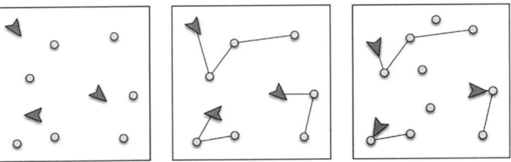
1-1 An illustration of dynamic routing problems for a robotic system. Panel #1: demands are generated. Panel #2: vehicles are assigned to demands and select routes. Panel #3: the DVR problem is how to recompute partitions and routes when new demands appear. . . . . 16 1-2 Example where re-optimization causes a vehicle to travel forever without
providing service to any demand. The vehicle is represented by a blue chevron object, a newly arrived demand is represented by a black circle, and old demands are represented by grey circles. . . . .. 17
2-1 Voronoi diagrams and power diagrams. . . . . 26
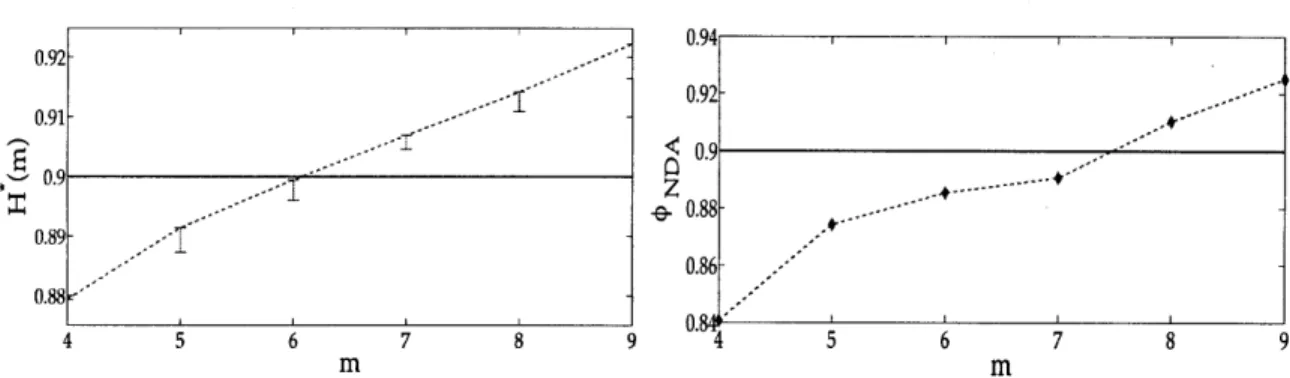
3-1 A cycle with Li = 4. . . . . 43 3-2 Left Figure: Approximate values for R*, (the bars indicate the range of values
obtained by maximizing Rm). Right Figure: Experimental values of
#NDA-The desired success factor is
#d
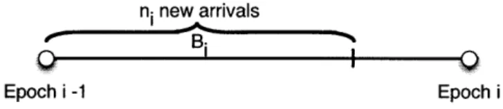
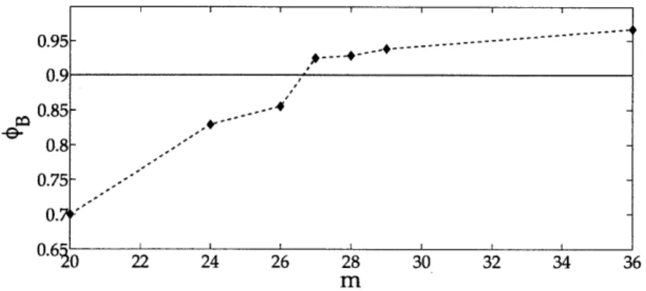
= 0.9. . . . . 52 3-3 Definition of epoch and busy period for the Batch policy. . . . . 543-4 Experimental values of
#B.
The desired success factor is#d
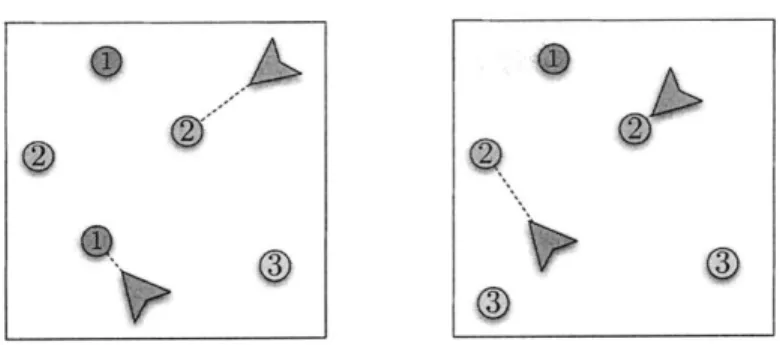
= 0.9. . . . . . 564-1 A depiction of the problem for two vehicles and three priority classes. Left
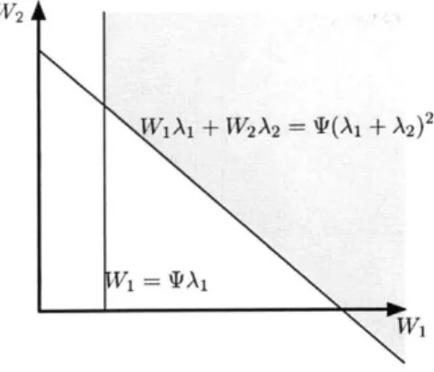
figure: One vehicle is moving to a class 1 demand, and the other to a class 2 demand. Right figure: The bottom vehicle has serviced the class 1 demand and is moving to a class 2 demand. A new class 3 demand has arrived. . . . 61 4-2 The feasible region of the linear program for 2 queues. When class 1 is of
higher priority, the solution is given by the corner. Otherwise, the solution is - oc . . . . 63 4-3 A representative simulation of the SQ policy for one vehicle and two priority
classes. Circle shaped demands are high priority, and diamond shaped are low priority. The vehicle is marked by a chevron shaped object and TSP tour is shown in a solid line. The left figure shows the vehicle computing a tour through class 1 demands. The center figure shows the vehicle part-way through the class 1 tour and some newly arrived class 2 demands. The right figure shows the vehicle after completing the class 1 tour and computing a new tour through all class 2 demands. . . . . 66 4-4 The tube heuristic for two classes of demands with c = 0.8, A2 = 6A1, and
several different load factors y. The system time at E = 0 corresponds to the
basic SQ policy. . . . . 75 4-5 Experimental results for the SQ policy in worst-case conditions plotted on a
4-6 The ratios upbdc/upbdpt for 2 classes of demands. . . . . 78
4-7 Ratio of experimental system times between Complete Merge policy and SQ policy as a function of A2, with n = 2, A1 = 1, c = 0.995 and o = 0.9. ... 79
5-1 A bipartite matching tour. The square represents the current location of the
vehicle. P1, P2, P3 are pick-up locations and D1, D2, D3 are the corresponding
delivery locations. Solid arrows show links between pick-up and delivery sites. Dotted arrows show links obtained by the bipartite matching between delivery and pick-up sites. Finally, dashed arrows show the primary tour
(TSP) through pick-up sites. The bipartite matching tour is: DPT -> Pi -*
D1 ->
P2 -+ D2-> P1 ->
P2 -> P3-
D--
> P-> DPT. . . . .
88
5-2 Performance of RB policy and comparison with upper and lower bounds.Left figure: TRB versus P. Right figure: scaling of TRB with respect to m. . 94
6-1 Equitable partitions by sweeping and slicing (assuming a uniform measure
f).102
6-2 Construction used for the proof of existence of equitable power diagrams. 103 6-3 Example of non-existence of an equitable Voronoi diagram on a line. The
above tessellation is an equitable partition, but not a Voronoi diagram. . . . 110
6-4 Gain function used to avoid that the positions of two power generators can coincide. . . . . 113 6-5 Typical equitable partitions achieved by using control law (6.22). The
yel-low squares represent the position of the generators, while the blue circles represent the centroids. Notice how each bisector intersects the line segment joining the two corresponding power neighbors almost at the midpoint; hence
both partitions are very close to Voronoi partitions. Compare with Figure 6-1.119
7-1 Left Figure: Ratio between experimental system time under the DC policy and
T*
(whose expression is given in equation (2.11)) in the case of uniform density (i.e., 6 = 0.9). Right Figure: Ratio between experimental system timeunder the DC policy and T* in the case of non-uniform density (6 = 0.6).
Circles correspond to the DC policy with r = 1, while squares correspond to
the DC policy with r = 16. . . . . 142
7-2 Left Figure: Ratio between experimental system time under the RH policy
and
T*
(whose expression is given in equation (2.11)) in the case of uniform density (i.e., 6 = 0.9). Right Figure: Ratio between experimental system timeunder the RH policy and TU in the case of non-uniform density (6 = 0.6). 143
7-3 The circles represent the ratios between the experimental system times under
the m-DC policy (with r = 1) and
T*
; the squares represent the theoretical upper bounds on these ratios. The load factor is p = 0.9 . . . . 144List of Tables
4.1 A comparison between the expected system time of the basic SQ policy,
and the SQ policy with the tube heuristic. The values in brackets give the
standard deviation of the corresponding table entry. . . . . 76
4.2 Ratio x between experimental results and upper bound for various values of g. 76 4.3 Ratio of upper bound with p, = c, for each a E {1, ... , n} and the upper bound with a locally optimized probability assignment . . . . 78
6.1 Performance of control law (6.22). . . . . 118
7.1 Adaptive policies for the 1-DTRP . . . . 122
7.2 Distributed and adaptive policies for the m-DTRP . . . . 122
Chapter 1
Introduction
This thesis presents a joint algorithmic and queueing approach to the design of cooperative control and task allocation strategies for networks of uninhabited vehicles and robots. The approach enables groups of robots to complete tasks in uncertain and dynamically changing environments, where new task requests are generated in real-time. Applications include surveillance and monitoring missions, as well as transportation networks and automated material handling.
As a motivating example, consider the following scenario: a sensor network is deployed in order to detect suspicious activity in a region of interest. (Alternatively, the sensor network is replaced by a a high-altitude sensor-rich aircraft loitering over the region.) In addition to the sensor network, a team of unmanned aerial vehicles (UANs) is available and each UAV is equipped with close-range high-resolution on-board sensors. Whenever a sensor detects a potential event, a request for close-range observation by one of the UAVs is generated. In response to this request, a UAV visits the location to gather close-range information and investigate the cause of the alarm. Each request for close-range observation might include priority levels or time windows during which the inspection must occur and it might require an on-site service time. In summary, from a control algorithmic viewpoint, each time a new request arises, the UAVs need to decide which vehicle will inspect that location and along which route. Thus, the problem is to design algorithms that enable real-time task allocation and vehicle routing.
Accordingly, this thesis presents allocation and routing algorithms that typically blend ideas from receding-horizon resource allocation, distributed optimization, combinatorics and control. The key novelty in our approach is the simultaneous introduction of stochastic, combinatorial and queueing aspects in the distributed coordination of robotic networks.
1.1
Static and Dynamic Vehicle Routing
In the recent past, considerable efforts have been devoted to the problem of how to coop-eratively assign and schedule demands for service that are defined over an extended geo-graphical area [69, 89, 2, 11, 6]. In these papers, the main focus is in developing distributed algorithms that operate with knowledge about the demand locations and with limited com-munication between robots. However, the underlying mathematical model is static, in that no new demands arrive over time, and fits within the framework of the static vehicle routing problem (see [99] for a thorough introduction to this problem), whereby: (i) a team of m vehicles is required to service a set of n demands in a 2-dimensional space; (ii) each demand
Figure 1-1: An illustration of dynamic routing problems for a robotic system. Panel #1: demands are generated. Panel #2: vehicles are assigned to demands and select routes. Panel #3: the DVR problem is how to recompute partitions and routes when new demands appear.
requires a certain amount of on-site service; (iii) the goal is to compute a set of routes that optimizes the cost of servicing (according to some quality of service metric) the demands. In general, most of the available literature on routing for robotic networks focuses on static environments and does not properly account for scenarios in which dynamic, stochastic and
adversarial events take place.
The problem of planning routes through service demands that arrive during a mission execution is known as the "dynamic vehicle routing problem" (abbreviated as the DVR problem in the operations research literature). There are two key differences between static and dynamic vehicleerouting problems. First, planning algorithms should actually provide
policies (in contrast to pre-planned routes) that prescribe how the routes should evolve as a
function of those inputs that evolve in real-time. Second, dynamic demands (i.e., demands that arrive and vary over time) add queueing phenomena to the combinatorial nature of vehicle routing. In such a dynamic setting, it is natural to focus on steady-state performance instead of optimizing the performance for a single task. Additionally, system stability in terms of the number of waiting demands is an issue to be addressed.
1.2
Algorithmic Approaches to DVR Problems
Broadly speaking, there are three main approaches available in the literature to tackle DVR problems. The first approach is to simply re-optimize every time a new event takes place; we call this approach "one-step sequential optimization". In the second approach, called "online algorithms", routing policies are designed to minimize the worst-case ratio between their performance and the performance of an optimal offline algorithm which has a priori knowledge of the entire input sequence. In the third approach, which we call "algorithmic queueing theory", the routing problem is embedded within the framework of queueing theory and routing policies are designed to minimize typical queueing-theoretical cost functions such as the expected waiting time in the system for the demands. In this section we review the three aforementioned approaches and we motivate our choice to use a queueing-theoretical framework to study DVR problems for robotic networks.
1.2.1 One-Step Sequential Optimization
A naive approach to DVR is to re-optimize every time a new demand arrives, by using an
algorithm that is optimal for the corresponding static vehicle routing problem. However,
0 0.5 1
(a) A new demand arrives at x = 1.
0 0.5 1
(b) A new demand arrives at x = 0 just before the
vehicle reaches x = 0.5.
a 0.5 1 0 0.33 0.5 1
(c) The vehicle re-optimizes its route and reverses (d) A new demand arrives at x = 1 and the vehicle
its motion. after re-optimizing reverses its motion
Figure 1-2: Example where re-optimization causes a vehicle to travel forever without pro-viding service to any demand. The vehicle is represented by a blue chevron object, a newly arrived demand is represented by a black circle, and old demands are represented by grey circles.
this approach can lead to highly undesirable behaviors as the following example shows. Assume that a unit-velocity vehicle provides service along a line segment of unit length (see Figure 1-2(a)). New demands arrive either at endpoint x = 0 or at endpoint x = 1. Assume that the objective is to minimize the average waiting time of the demands (as it is common in the DVR literature); hence a re-optimization algorithm provides a route that minimizes J:', Wj, where n is the number of outstanding demands at that time, and W, is the waiting time for the jth demand. Assume that at time 0 the vehicle is at x = 0
and a new demand arrives at x = 1. Hence, the vehicle travels immediately toward that
demand. Assume that just before reaching x = 1/2 a new demand arrives at x = 0. It is
easy to show that the optimal strategy is to reverse motion and provide service first to the demand at x = 0. However, assume that just before reaching x = 1/3 a new demand arrives
at x = 1. It is easy to show that the optimal strategy is to reverse motion and provide
service first to the demands at x = 1. In general, let k, n be positive integers and let
Ek = k/(2k ± 1). Assume that just before time t2n- 1 = 1/2 +
Zn-(1
- 2ek) a new demandarrives at x = 0, and that just before time t2n = t2 n-1 + 1/2 - En a new demand arrives at
x = 1. (Assume that at time to = 0 the vehicle is at x = 0 and a new demand arrives at x = 1.) It is possible to show that at each new arrival the optimal strategy ensuing from a
re-optimization algorithm is to reverse motion before one of the two endpoints is reached. Note that lim,+,o tn = +oo, hence the vehicle will travel forever without servicing any
demand!
This example therefore illustrates the pitfalls of the straightforward application of static routing and sequential re-optimization algorithms to dynamic problems. Broadly speaking, we argue that DVR problems require tailored routing algorithms with provable performance guarantees. There are currently two main algorithmic approaches that allow both a rigorous synthesis and an analysis of routing algorithms for DVR problems; we review these two approaches next.
1.2.2
Online Algorithms
An online algorithm is one that operates based on input information given up to the current time. Thus, these algorithms are designed to operate in scenarios where the entire input is not known at the outset, and new pieces of the input should be incorporated as they become available. The distinctive feature of the online algorithm approach is the method that is used to evaluate the performance of online algorithms, which is called competitive
analysis [88]. In competitive analysis, the performance of an online algorithm is compared
to the performance of a corresponding offline algorithm (i.e., an algorithm that has a priori knowledge of the entire input) in the worst case scenario. Specifically, an online algorithm is c-competitive if its cost on any problem instance is at most c times the cost of an optimal offline algorithm:
COstonline (I) C COStoptimal offline(I), V problem instances I.
In the recent past, dynamic vehicle routing problems have been studied in this frame-work, under the name of the online traveling repairman problem [56, 49, 523.
While the online algorithm approach applied to DVR has led to numerous results and interesting insights, it leaves some questions unanswered, especially in the context of robotic networks. First, competitive analysis is a worst-case analysis, hence, the results are often overly pessimistic for normal problem instances. Moreover, in many 'applications there is some probabilistic problem structure (e.g., spatial distribution of future demands), that can be advantageously exploited by the vehicles. In online algorithms, this additional information is not taken into account. Second, competitive analysis is used to bound the performance relative to the optimal offline algorithm, and thus it does not give an absolute measure of performance. In other words, an optimal online algorithm is an algorithm with minimum "cost of causality" in the worst-case scenario, but not necessarily with the minimum worst-case cost. Finally, many important real-world constraints for DVR, such as time windows, priorities, and pick-up/delivery locations "have so far proved to be too complex to be considered in the online framework" [45, page 2061. Some of these drawbacks have been recently addressed by [100}, where a combined stochastic and online approach is proposed for a general class of combinatorial optimization problems and is analyzed under some technical assumptions.
This discussion motivates an alternative approach for DVR in the context of robotic networks, based on probabilistic modeling, and average-case analysis.
1.2.3
Algorithmic Queueing Theory
Algorithmic queueing theory embeds the dynamic vehicle routing problem within the frame-work of queueing theory and overcomes most of the limitations of the online algorithm ap-proach; in particular, it allows to take into account several real-world constraints, such as time constraints and priorities. We call this approach algorithmic queueing theory since its objective is to synthesize an efficient control policy, whereas in traditional queueing theory the objective is usually to analyze the performance of a specific policy. Here, an efficient policy is one whose expected performance is either optimal or optimal within a constant factor.1 Algorithmic queueing theory consists of the following steps:
'The expected performance of a policy is the expected value of the performance over all possible inputs (i.e., demand arrival sequences). A policy performs within a constant factor r, of the optimal if the ratio between the policy's expected performance and the optimal expected performance is upper bounded by r,.
1. queueing model of the robotic system and analysis of its structure;
2. establishment of fundamental limitations on performance, independent of algorithms; and
3. design of algorithms that are either optimal or constant-factor away from optimal,
possibly in specific asymptotic regimes.
Finally, the proposed algorithms are evaluated via numerical, statistical, and experimental studies, including Monte Carlo comparisons with alternative approaches.
In order to make the model tractable, demands are usually considered "statistically independent" and their arrival process is assumed stationary (with possibly unknown pa-rameters). Because these assumptions can be unrealistic in some scenarios, this approach has its own limitations. Pioneering work in this context is that of Bertsimas and Van Ryzin [14, 15, 16], who introduced queueing methods to solve the simplest DVR problem (a vehicle moves along straight lines and visits demands whose time of arrival, location and on-site service are stochastic; information about demand location is communicated to the vehicle upon demand arrival); see also the earlier related work [84].
One of the fundamental contributions of this thesis is to show that algorithmic queue-ing theory, despite the aforementioned disadvantages, is a very useful framework for the design of routing algorithms for robotic networks and a valuable complement to the online algorithm approach.
1.3
Contributions of the Thesis
The objective of this thesis is to develop a joint algorithmic and queueing approach to the design of cooperative control and task allocation strategies for networks of uninhabited
vehicles required to operate in dynamic and uncertain environments. By leveraging on the algorithmic queueing theory approach introduced in [14, 15, 16] and integrating ideas from dynamics, combinatorial optimization, probability theory, and distributed algorithms, we develop a systematic approach to tackle complex dynamic routing problems for robotic networks. The power of algorithmic queueing theory stems from the wide spectrum of aspects, critical to the routing of robotic networks, for which it enables a rigorous study; specific examples taken from this thesis include complex models for the demands such as time constraints, service priorities, and pick-up/delivery locations, and problems concerning robotic implementation such as adaptivity and decentralized computation.
It is important to emphasize that many of the routing policies proposed in this thesis can not be analyzed by using standard techniques in queueing theory (this is due to the fact the the travel times introduce correlations among the service times for the demands); hence in this dissertation we also introduce novel analysis techniques that merge ideas from control theory and combinatorics and that are interesting in their own right.
This thesis is divided into two parts. The first part, which includes chapters 3, 4, and 5, deals with the application of algorithmic queueing theory to DVR problems with complex demand models. The second part includes chapters 6 and 7, and deals with the study of vehicle routing policies that are specifically tailored to large-scale robotic networks. The contributions of each chapter can be summarized as follows.
Chapter 2: Preliminaries. In this chapter we first introduce some notation. Then, we review some basic results in probability theory, computational geometry, locational
optimization and combinatorics on which we will rely throughout the thesis. Finally, we review the m-vehicle Dynamic Traveling Repairman Problem, which paved the way for the algorithmic queueing theory approach.
Chapter 3: DVR with Stochastic Time Constraints. In this chapter we study time-constrained DVR problems where demands have deadlines on their waiting times. Surprisingly, little is known about time-constrained versions of DVR problems, despite their practical relevance. The purpose of this chapter is to fill this gap. Specifically, we study the following problem: m vehicles operating in a bounded environment and traveling with bounded velocity must service demands whose time of arrival, location and on-site service are stochastic; moreover, once a demand arrives, it remains active for a (possibly stochastic) amount of time, and then expires. An active demand is successfully serviced when one of the vehicles visits its location before its deadline and provides the required on-site service. The aim is to find the minimum number of vehicles needed to ensure that the long-time fraction of demands that are successfully serviced is larger than a desired value
#d
E (0, 1), and to determine the policy thevehicles should execute to ensure that such objective is attained. Our contributions are threefold. First, we carefully formulate this problem by also taking into account the possible types of available information (e.g., the deadlines). In setting up the problem, we prove some ergodicity results that are interesting in their own right. Second, by using a variety of techniques from geometric probability, we establish a lower bound on the optimal number of vehicles for a given level of service quality (i.e.,
#d).
In deriving the lower bound, we introduce a novel type of facility location problem, which we call the m-Location Problem with Impatient Customers (m-LPIC), and for which we provide some analysis and algorithms. Third, we analyze two service policies: we (i) show that one of the proposed policies is optimal in light load (i.e., when the arrival rate is small); (ii) derive an analytical upper bound on the number of vehicles needed by one of the two policies to achieve a given service quality; (iii) find that if the on-site service requirement is "negligible", the minimum number of vehicles isO(vN),
where A is the arrival rate for the demands; (iv) prove that one of the proposed policies is within a small factor of the optimal when <d is close to one, the system is in heavy load (i.e., the arrival rate is large), and the deadlines are deterministic.Chapter 4: DVR with Priority Classes. In this chapter we study a DVR problem in
which there are multiple priority classes of service demands. Demands belonging to multiple priority classes arrive in the environment randomly over time and require a random amount of on-site service that is characteristic of the class. To service a demand, one of m vehicles must travel to the demand location and remain there for the required on-site service time. The quality of service provided to each class is given by the expected delay between the arrival of a demand in the class, and that demand's service completion. The goal is to design a routing policy for the service vehicles which minimizes a convex combination of the delays for each class. This problem has important applications in areas such as UAV surveillance, where targets are given different priority levels based on their urgency or potential importance [11]. First, we derive a lower bound on the achievable values of the convex combination of delays. Second, we propose a novel policy, which we call SQ policy, in which each class of demands is served separately from the others. We show that in heavy load
the policy performs within a constant factor 2n2 of the lower bound, where n is the number of classes. Thus, the constant factor is independent of the number of vehicles, the arrival rates of demands, the on-site service times, and the convex combination coefficients. Finally, we present an improvement on the SQ policy in which classes of similar priority are merged together. We also perform extensive simulations and introduce an effective heuristic improvement called the tube heuristic.
Chapter 5: DVR in Transportation Systems. Transportation on demand (TOD)
sys-tems, where users generate requests for transportation from a pick-up point to a deliv-ery point, are already vdeliv-ery popular and are expected to increase in usage dramatically as the inconvenience of privately-owned cars in metropolitan areas becomes excessive. Routing service vehicles through customers is usually accomplished with heuristic algorithms. In this chapter we study TOD systems in the form of a unit-capacity, multiple-vehicle dynamic pick-up and delivery problem, whereby pick-up requests ar-rive according to a Poisson process and are randomly located according to a general probability density. Corresponding delivery locations are also randomly distributed according to a general probability density, and a number of unit-capacity vehicles must transport demands from their pick-up locations to their delivery locations. First, we derive insightful fundamental bounds on the steady-state waiting times for the de-mands, and then we devise constant-factor optimal dynamic routing policies that rely on the repeated solution of traveling salesman and bipartite matching problems.
Chapter 6: Spatially Distributed Algorithms for Environment Partitioning. The
best previously known control policies for DVR problems rely on centralized task as-signment and are not robust against changes in the environment, in particular changes in load conditions; therefore, they are of limited applicability in scenarios involving ad hoc networks of autonomous vehicles operating in a time-varying environment. In this chapter, by blending ideas from algebraic topology and control theory, we devise spatially distributed algorithms for environment partitioning that will be piv-otal to design distributed routing policies for DVR problems. The application of the algorithms developed in this chapter to DVR problems is discussed in chapter 7. The distributed partitioning algorithms we present in this chapter are indeed useful beyond their application to DVR problems, since they allow a mobile robotic network to equitably share the workload among its members in a wide variety of scenarios.
Chapter 7: Adaptive and Distributed Algorithms for DVR. In this chapter we
lever-age on the spatially distributed algorithms developed in chapter 6 to obtain adaptive and distributed algorithms for DVR problems, in particular for the m-vehicle Dynamic Traveling Repairman Problem (m-DTRP).
Specifically, the contributions of this chapter are as follows. First, we present a new class of unbiased policies for the 1-DTRP. In particular, we propose the Divide & Conquer (DC) policy, whose performance depends on a design parameter r E N. If r --
+oc,
the policy is (i) provably optimal both in light- and in heavy-load conditions, and (ii) adaptive with respect to changes in the load conditions and in the statistics of the on-site service requirement; if, instead, r = 1, the policy is (i) provably optimal inlight-load conditions and within a factor 2 of the optimal in heavy-load conditions, and (ii) adaptive with respect to all problem data, in particular, and perhaps surprisingly, it does not require any knowledge about the demand generation process. Moreover,
by applying ideas of receding-horizon control to dynamic vehicle routing problems, we
introduce the Receding Horizon (RH) policy, that also does not require any knowledge about the demand generation process; we show that the RH policy is optimal in light-load and stable in any light-load condition, and we heuristically argue that its performance is close to optimal in heavy-load conditions (in particular, we heuristically argue that the RH policy is the best available unbiased and adaptive policy for the
1-DTRP). Second, we show that specific partitioning policies, whereby the environment is partitioned among the vehicles and each vehicle follows a certain set of rules in its own region, are optimal in heavy-load conditions. Finally, by combining the DC policy with the spatially distributed algorithms for environment partitioning developed in chapter 6, we design a routing policy for the m-DTRP (called m-DC policy) that (i) is spatially distributed, scalable to large networks, and adaptive to network changes, (ii) is within a constant-factor of the optimal performance in heavy-load conditions (in particular, it is optimal when demands are uniformly dispersed over the environment or when the average on-site service time requirement is negligible) and stabilizes the system in any load condition. Here, by network changes we mean changes in the number of vehicles, in the arrival rate of demands, and in the characterization of the on-site service requirement.
Chapter 8: Conclusion In this final chapter we draw our conclusions, and present some
Chapter 2
Preliminaries
In this chapter we first introduce some notation. Then, we review some basic results in probability theory, computational geometry, locational optimization and combinatorics on which we will rely throughout this thesis. Concepts that, instead, are specific to single chapters will be presented at the beginning of those chapters. Finally, we review the m-vehicle Dynamic Traveling Repairman Problem, which paved the way for the algorithmic queueing theory approach.
2.1
Notation
We let No, N, R, R>o, and R>o denote the set of nonnegative integers, the set of positive integers, the set of real numbers, the set of nonnegative reals number, and the set of positive reals numbers, respectively. Let ||-|| denote the Euclidean norm. Let
8
be a compact, convex subset of Rd, d E N. We denote the boundary of E as&E
and the Lebesgue measure of S as|1. We define the diameter of
8
as: diam(E) sup{j|p - qj Ip, qC
E}. The distance froma point x to a set S is defined as dist(x, S) infPes |x - p|. We define Im = {1, 2,. .. Im}.
Let G = (gi, ... , gm) c Em denote the location of m points.
For h, g : N -> R>o, we say that h E O(g) (resp., h E Q(g)) if there exist no E N and
K E R>o (resp., k E R>o) such that h(n) <; Kg(n) for all n > no (resp., h(n) kg(n) for
all n > no). If h E O(g) and h
c
Q(g), then we use the notation hc
0(g).2.2
Some Basic Definitions and Facts in Probability Theory
If X and Y are two random variables defined on the same probability space, then X is almost
surely larger than Y if and only if P [X > Y] = 1; X is surely larger than Y if and only if
X(w) Y(w) for all samples w E Q, with Q being the sample space. A sequence of random
variables
{Yj; j
C No} converges almost surely to a random variable Y if and only if the event{w E Q: limj+o Yj(w) = Y(w)}, where Q is the sample space, has probability 1. For any
nonnegative, real-valued random variable Y, one can show that E [Y] =
f+
P [Y > y] dy. Suppose h(.) is a convex function and Y is a random variable, then Jensen's inequality states that E [h(Y)] ;;, h(E [Y]), provided both expectations exist. Finally, if X is an integrable random variable (i.e., a random variable satisfying E [IXI] < +oo) and Y is any random variable, not necessarily integrable, on the same probability space, then E [X] = E [E [XIY]].2.3
Computational Geometry
2.3.1 Partitions
Let E c Rd be a bounded, convex set. An m-partition of S (where m
C
N) is a collectionof m closed subsets {Ek}g 1 with disjoint interiors, whose union is F. A partition {Ek}1 i
is convex if each Ek is convex.
2.3.2 Equitable partitions
Given a measurable function
f
: E -* R>o, an m-partition {Ek}lg is equitable with respect tof
iff,
f (x) dx =fe
f(x) dx/m for all k E {l,... , m}. Similarly, given two measurablefunctions
f
3 :8F -+ R>o,j
E {1, 2}, an m-partition {Ek}l 1 is simultaneously equitable withrespect to fi and
f
2 if fek f,(x) dx = fe f,(x) dx/m for all k E {1..., m} and j c {1, 2}.Theorem 12 in [171 and Corollary 3 in
[851
show that, given two measurable functionsfj
: E -> R>o,j
C {1, 2}, there always exists an m-partition of E that is simultaneouslyequitable with respect to f1 and f2 and where the subsets Ek are convex.
2.3.3
Voronoi diagrams and power diagrams
We refer the reader to [721 and [48} for comprehensive treatments, respectively, of Voronoi diagrams and power diagrams, which are special types of partitions. Assume, first, that G is an ordered set of distinct points in S. The Voronoi diagram V(G) = (Vi(G), ... , Vm(G))
of S generated by points G = (g1,... , gm) is defined by
Vi(G)
={x E El ||x
-gil
lx
-gj||,
Vj = i,j E
Im}. (2.1) We refer to G as the set of generators of V(G), and to Vi(G) as the Voronoi cell or region of dominance of the ith generator. For gi, gj c G, i = j, we define the bisector between giand gj as b(gi, gj) = {x
c
l
I[x
-
gi
H =
lx
- gj l}. The face b(gi, gj) bisects the line segment
joining gi and gj, and this line segment is orthogonal to the face (Perpendicular Bisector
Property). The bisector divides E into two convex subsets, and leads to the definition of
the set D(gi, gj) = {x E
1 Ilx
- gil1 kz
- g11};
we refer to D(gi, gj) as the dominanceregion of gi over gj. Then, the Voronoi partition V(G) can be equivalently defined as
Vi(G) =
A
EIm\{i} D(gi, gj). This second definition clearly shows that each Voronoi cell isa convex set. Indeed, a Voronoi diagram of E is a convex partition of 8 (see Figure 2-1(a)). The Voronoi diagram of an ordered set of possibly coincident points is not well-defined. We define
'coine= {(91, - --,gm) E Em |gi = gj for some i
$
j E {1, .. .,m}}. (2.2)Assume, now, that each point gi E G has assigned an individual weight Wi E R, i E Im
let W = (wi, ... , wm). We define the power distance
dp(x,gi;wi) x-gif2 -Wi. (2.3)
We refer to the pair (gi, wi) as a power point. We define
Gw= ((gir cind) (gm, WM))f-
that Gw is an ordered set of distinct power points. Similarly as before, the power diagram
V(Gw) - (Vi(Gw), . . ., Vm(Giw)) of E generated by power points ((gi, wi),..., (gm, WM)) is defined by
V(Gw) =
{x
E Ello
-gCIl
- Wili
-gill
2 -g, VJ i, j E Im}. (2.4)We refer to Gw as the set of power generators of V(Gw), and to Vi(Gw) as the power cell or region of dominance of the ith power generator; moreover we call gi and wi, respectively, the position and the weight of the power generator (gi, wi). Notice that, when all weights are the same, the power diagram of 5 coincides with the Voronoi diagram of S. As before, power diagrams can be defined as intersection of convex sets; thus, a power diagram is, as well, a convex partition of S. Indeed, power diagrams are the generalized Voronoi diagrams that have the strongest similarities to the original diagrams [81. There are some differences, though. First, a power cell might be empty. Second, gi might not be in its power cell (see Figure 2-1(b)). Finally, the bisector of (gi, wi) and (g, wj), i
$
j, isb((gi,wi),(gj,wj)) = {x
c
E|
(gj - gi)TX =(1g1
-l1g,112
+ w, -wj)}. (2.5)Hence, b((gi, wi), (gj, wj)) is a face orthogonal to the line segment gj gj and passing through the point gf, given by
Igj||2
-ig, 112
+ 1 - w (gj - gi);g'i
2||gg - gilwi
this last property means that, by changing weights, it is possible to arbitrarily move the bi-sector between the positions of two power generators, while still preserving the orthogonality constraint.
The power diagram of an ordered set of possibly coincident power points is not well-defined. We define
Fcoinc =
{Gw
E (9 x R)m I g = gj and wi = wj for some i =j
E {1, m}}. (2.6)Notice that we used the same symbol as in equation (2.2): the meaning will be clear from the context.
For simplicity, we will refer to Vi(G) (Vi(Gw)) as Vi. When the two Voronoi (power) cells V and V are adjacent (i.e., they share a face), gi ((gi, wi)) is called a Voronoi (power)
neighbor of g, ((gj, wj)), and vice-versa. The set of indices of the Voronoi (power) neighbors
of gi ((gi, wi)) is denoted by Ni. We also define the (i, j)-face as Aij = Vi
n
V.2.3.4
The continuous multi-median problem
Given a set S C Rd and a vector G = (g1,... , gin) of m distinct points in S, the expected
distance between a random point x, generated according to a probability density function
f,
and the closest point in G is given byHm(GS)= E min 1g9 - = E 1gk -xIf(x)dx,
(a) A Voronoi Diagram. (b) A power diagram. The weights wi
are assumed positive. The radii of cir--cles represent the magnitudes of weights. Power generator (g2, W2) has an empty
cell. Power generator (g5, W5) is outside
its region of dominance. Figure 2-1: Voronoi diagrams and power diagrams.
where V(G) = (V1I(G),..., Vm(G)) is the Voronoi partition of the set E generated by the
points G. The function Hm is known in the locational optimization literature as the con-tinuous Weber function or the concon-tinuous multi-median function; see [1, 391 and references therein.
The m-median of the set E, with respect to the measure induced by
f,
is the global minimizerG* (E) = arg min Hm(G, E).
GEEm
We let H*,(E) = Hm(G* (E), E) be the global minimum of Hm. It is straightforward to
show that the map G '- H1 (G, E) is differentiable and strictly convex on E. Therefore, it
is a simple computational task to compute G* (E). It is convenient to refer to G* (E) as the median of E. On the other hand, when m > 1, the map G '-4 Hm(G, E) is differentiable
(whenever (gi,... , gm) are distinct) but not convex, thus making the solution of the con-tinuous m-median problem hard in the general case. It is known [1, 651 that the discrete version of the m-median problem is NP-hard for d > 2. The set of critical points of Hm contains all configurations (gi, . .. , gm) with the property that each point gA is the generator of the Voronoi cell Vk(G) as well as the median of Vk(G) (we refer to such Voronoi diagrams as median Voronoi diagrams); in particular, the global minimum of Hm must be one of these configurations.
2.4
Combinatorics
2.4.1
The traveling salesman problem in the Euclidean plane
The Euclidean Traveling Salesman Problem (for short, TSP) is formulated as follows: given a set
Q
of n points in Rd, find a minimum-length tour (i.e., a cycle that visits all nodes exactly once) ofQ;
the length of a tour is the sum of all Euclidean distances on the tour. LetTSP(Q) denote the minimum length of a tour through all the points in
Q;
by convention, TSP(0) = 0. Assume that the locations of the n points are random variables independentlyand identically distributed in a compact set E; in [96] it is shown that there exists a constant
3
TSP,d such that
lim E [TSP(Q)]
f
fll/d(X)dx,
(2.7)
n--++oO mi-l/d 3 s~i
where
f
is the density of the absolutely continuous part of the point distribution. For the case d = 2, the constant#TSP,2
has been estimated numerically as#TSP,2
~ 0.7120 +0.0002 [83]. The constant
#TSP,3
has been estimated numerically as#TSP,3
0.6979 ±0.0002, [83]. In this thesis we will refer to
#TSP,2
and#TSP,3
simply as#TSp:
the meaning will be clear from the context. Notice that the limit in equation (2.7) holds for all compact sets: the shape of the set only affects the convergence rate. According to [58], if E is a "fairly compact and fairly convex" set in the plane, then equation (2.7) provides a "good" estimate of the expected TSP tour length for values of n as low as 15.Remarkably, the asymptotic average cost of the stochastic TSP for uniform point distri-butions is an upper bound on the asymptotic average cost for general point distridistri-butions: i.e.,
E [TSP(Q)]
11dlim 1_ld < #TSP,d I
n-)+oo n/
where 1E| is the hypervolume of E; this follows directly from an application of Jensen's inequality to the concave function g(x) = Xzd~, x E R>O and d E N, in the right hand side
of (2.7)
1
jf 1|11d(x)
dx <
g1|/d ((x)
dx) d|
11/dFinally, for any bounded environment E, the following (deterministic) bound holds on the length of the TSP tour, uniformly on n [96]:
TSP(Q) :5,,0,d |Ell/d n' -1/d, (2.8)
where |E1 is the hypervolume of
.
and 3,,d
is a constant generally larger than 3TSP,d. Wewill refer to 13 ,d as the characteristic constant of 8.
2.4.2 The bipartite matching problem
Let
Q
be a set of points X1, ... , Xn, Y1,.. Yn that are i.i.d. in a compact set E c Rd,d ;> 3, and distributed according to a density
f.
Let BM(Q) = minIE"
I|Xj
- Yj(i) ||denote the optimal bipartite matching of the X and Y points, where a ranges over all permutations of the integers 1, 2,. .. , n. In [38] it is shown that there exists a constant /3M,d such that
lim E [BM(Q)]
f
11/d(x) dx. (2.9)n--+oo nl/d
The constant /M,3 has been estimated numerically as